Article

A New Semi-Analytical Method for Elasto-Plastic Analysis of a Deep Circular Tunnel Reinforced by Fully Grouted Passive Bolts

1
School of Civil Engineering, Southwest Jiaotong University, Chengdu 610036, China
2
Key Laboratory of Traffic Tunnel Engineering, Ministry of Education, Southwest Jiaotong University, Chengdu 610036, China
*
Authors to whom correspondence should be addressed.
Appl. Sci. 2020, 10(12), 4402; https://doi.org/10.3390/app10124402
Submission received: 18 May 2020 / Revised: 13 June 2020 / Accepted: 21 June 2020 / Published: 26 June 2020
(This article belongs to the Section Civil Engineering)

Abstract

:

Featured Application

The proposed model can be employed as a useful tool in the preliminary design and stability analysis of a tunnel reinforced by fully grouted passive bolts.

Abstract

The use of fully grouted passive bolts as a reinforcement technique has been widely applied to improve the stability of tunnels. To analyze the behaviors of passive bolts and rock mass in a deep circular tunnel, a new semi-analytical solution is presented in this work based on the finite difference method. The rock mass was assumed to experience elastic–brittle–plastic behavior, and the linear Mohr–Coulomb criterion and the nonlinear generalized Hoek–Brown criterion were employed to govern the yielding of the rock mass. The interaction and decoupling between the rock mass and bolts were considered by using the spring–slider model. To simplify the analysis process, a bolted tunnel was divided into a bolted region and an unbolted region, while the contact stress at the bolted–unbolted interface and the rigid displacement of the bolts were obtained using two boundary conditions in combination with the bisection method. Comparisons show that the results obtained using the proposed solution agree well with those from the commercial numerical software and the in situ test. Finally, parametric analyses were performed to examine the effects of various reinforcement parameters on the tunnel’s stability. The proposed solution provided a fast but accurate estimation of the behavior of a reinforced deep circular tunnel for preliminary design purposes.

1. Introduction

Rock bolts have been used in underground engineering to stabilize rock masses for more than 100 years [1]. At present, many kinds of rock bolts have been developed, among which, fully grouted passive bolts are the most popular type and have been widely employed due to their economical and convenient nature. The analytical solution for a deep circular tunnel reinforced with passive bolts in a hydrostatic field is a classical problem in underground engineering. Although the practicability of the analytical solutions is limited by their assumptions, they can be employed to quickly assess the mechanical behaviors of the rock mass and reinforcement and can be used for preliminary design analyses or the pre-dimensioning of the reinforcement [2,3].
By assuming that the rock mass and the passive bolts have the same strain—that is, no relative displacement occurs at the bolt–rock interface—a series of analytical and semi-analytical solutions were formulated by many authors [2,4,5,6,7,8,9,10,11,12,13] in terms of the elastic, viscoelastic, and elastoplastic rock mass, starting in the 1980s. However, according to the in situ test results reported by Freeman [14], the relative displacement between the bolts and rock mass is produced with the advance of the tunnel face, which results in shear stresses at the bolt–rock interface and induces a tension force in the bolts. In addition, Cui et al. [15] reported that this assumption causes an overestimation of the tensile force in the bolts and leads to an overly conservative design. Therefore, it is necessary to reasonably consider the interaction between the bolts and the rock mass.
To simplify this problem, an equivalent material method was developed by Indraratna and Kaiser [16,17] to consider a proper interaction mechanism, and the analytical solution for a reinforced deep circular tunnel in a Mohr–Coulomb rock mass is proposed. Osgoui and Oreste [18,19] and Osgoui and Ünal [20] improved this solution by incorporating the Hoek–Brown failure criterion to represent the rock mass behavior using a more rigorous assessment of the strain compatibility. However, these solutions determine the position of the neutral point of the passive bolts using an empirical equation [21] instead of a rigorous theoretical analysis. The empirical equation assumes that the position of the neutral point is only related to the tunnel radius and the bolt length, which is inconsistent with the results reported by Cai et al. [22,23] and Li and Stillborg [24], which state that the position of the neutral point is related to the properties of the bolts and rock mass.
The aforementioned studies show that it is quite difficult to derive an analytical solution to reasonably assess the interaction between passive bolts and the rock mass due to the complexity of this problem. Guan et al. [25], Oreste [26], and Tan [27,28] all proposed a semi-analytical solution of great interest; however, Guan et al. [25] mechanically defined the position of the neutral point and neglected the effect of the end plate. Oreste [26] modeled the shear distribution at the bolt–rock interface with a predefined interaction curve for the shear stress. Guan et al.′s and Oreste′s solutions are limited to the Mohr–Coulomb failure criterion. Moreover, in both Guan et al.′s and Tan′s solutions, the advance of the tunnel face is simulated using a gradually decreased support pressure from the initial stage to the final stage. In each intermediate stage, an iterative process is required to evaluate the mechanical behaviors of the passive bolts and rock mass; therefore, numerous stages are needed to ensure the accuracy of the analysis, which is cumbersome and time-consuming. Recently, Cui et al. [15,29] proposed an ingenious and improved semi-analysis solution by considering only the initial and final stages (i.e., no intermediate states); however, this solution is limited to the Mohr–Coulomb failure criterion and the behavior at the bolt–rock interface is assumed to be linear elastic for simplicity, which is inconsistent with experimental results showing that the decoupling generally occurs at the rock–bolt interface. This assumption may overestimate the reinforcement effectiveness of passive bolts and result in an unsafe design.
To overcome the above deficiencies, a new semi-analytical method was established in this study. Section 2 describes the behaviors of the passive bolts and the rock mass in a deep circular tunnel, as well as the basic equations. Section 3 presents the details of the semi-analytical solution. Section 4 verifies the proposed solution via comparisons with the results from the commercial numerical software FLAC3D (Version 5.0, Itasca Consulting Group, Inc., Minneapolis, MN, USA) and in situ tests. Section 5 discusses the model’s behavior with a series of parametric studies.

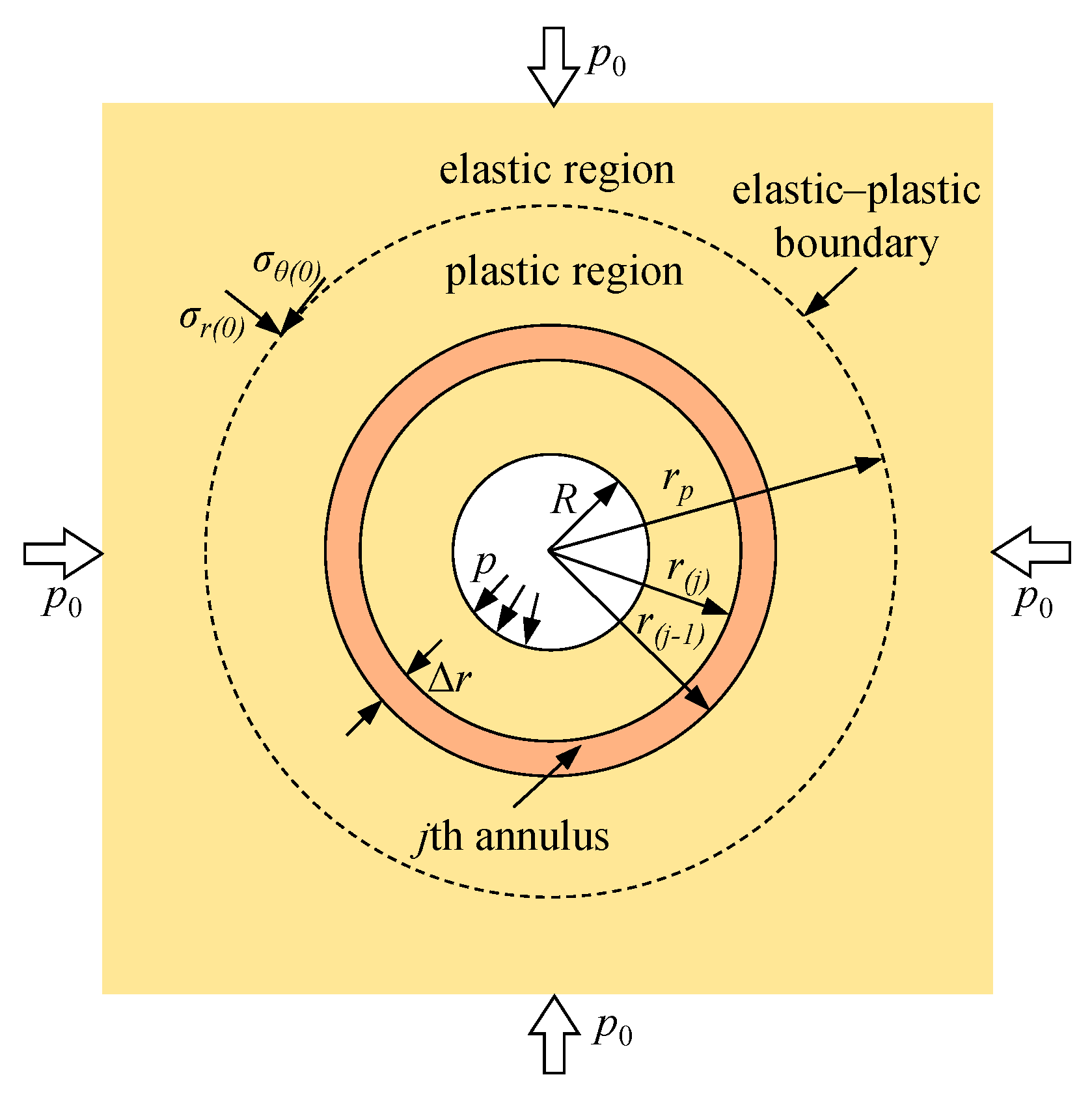
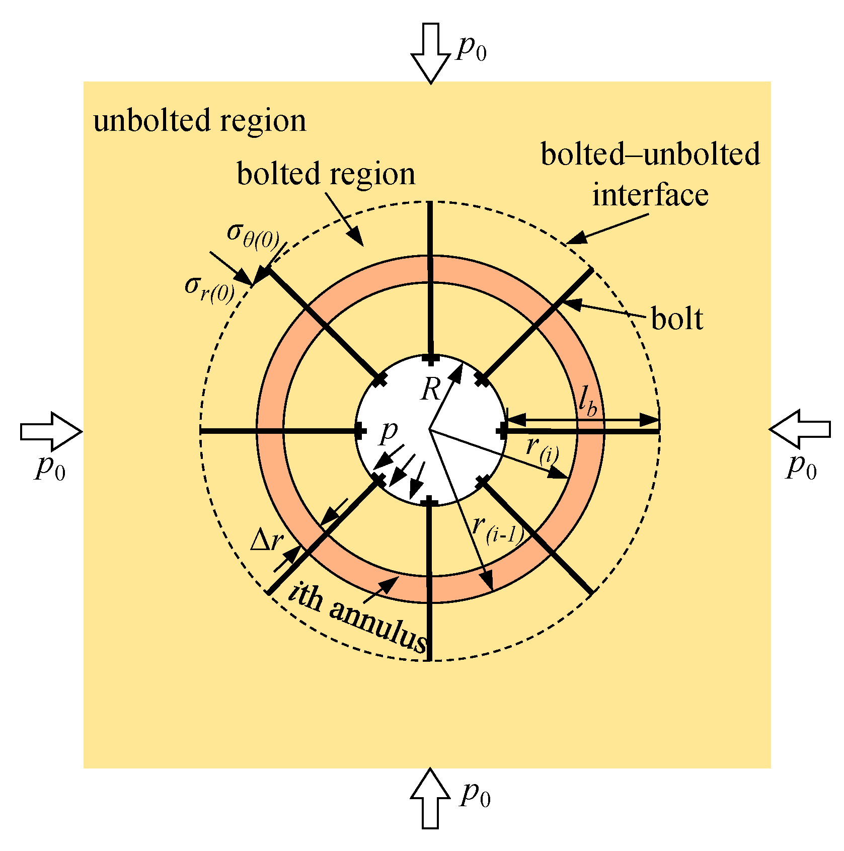
2. Definition of the Problem

2.1. Basic Assumptions

A reinforced deep circular tunnel is illustrated in Figure 1, and the following assumptions were made to solve this problem:
(1) Under the plane strain condition, a deep circular tunnel of radius R is excavated in an infinite isotropic, continuous, homogeneous, and elastoplastic rock mass with a hydrostatic stress field p0.
(2) The rock mass experiences elastic–brittle–plastic behavior, and the yielding of the rock mass is governed by the linear Mohr–Coulomb criterion or the nonlinear generalized Hoek–Brown criterion.
(3) The passive bolts with length lb are installed uniformly around the tunnel. In the transverse section perpendicular to the axis of the tunnel, the angle between two adjacent bolts is ω. In the longitudinal section parallel to the axis of the tunnel, the spacing between two adjacent bolts is lz. Therefore, the tributary area of each bolt is assumed to be lz (r denotes the radial distance in the rock mass to the tunnel center).

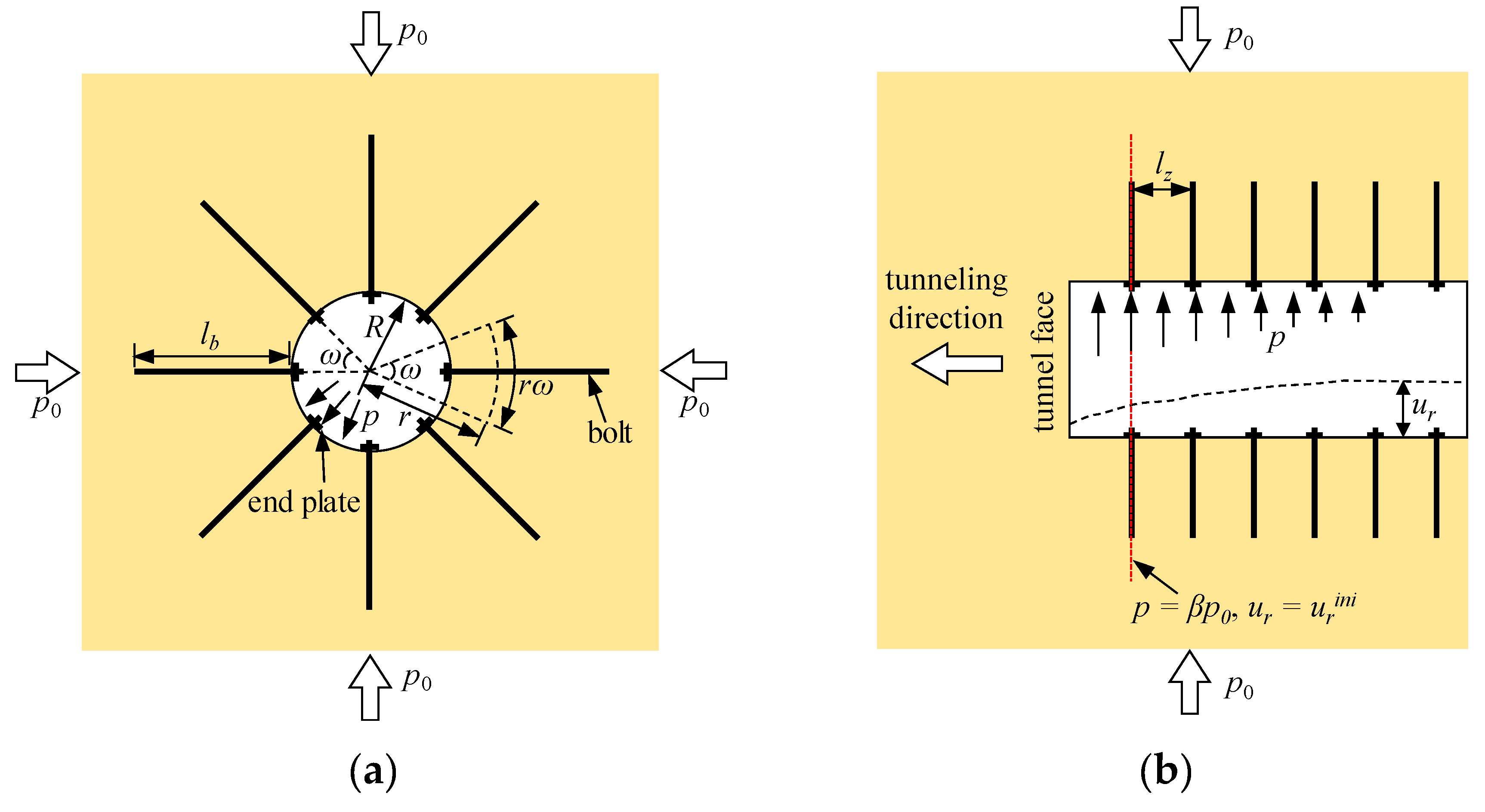
2.2. Tunnel Face Effect during Tunneling

As shown in Figure 1, a support pressure p is applied on the tunnel periphery by the tunnel face effect, and its value gradually decreases to 0 with the advance of the tunnel face. Therefore, due to the tunnel face effect, the behavior of a deep tunnel during tunneling is essentially a three-dimensional problem. The bolts are installed behind the tunnel face, where the support pressure is βp0 (β is the coefficient of the tunnel face effect) and the corresponding rock displacement is u r i n i (the initial radial displacement of the rock mass), while the bolts are yet to work at this moment. Then, the support pressure decreases during the advance of the tunnel, which leads to an increase of the radial displacement of rock mass ur and the interaction between the rock mass and bolts. The tunnel face effect can be approximated using the β-method.
The β-method consists of two steps: (1) the tunnel is excavated and a support pressure βp0 is applied to the tunnel periphery, and (2) the bolts are installed and the stress βp0 is shared by the ground and the bolts during the advance of the tunnel. The magnitude of β is related to the distance between the installation position and the tunnel face, where a large distance is associated with a small β and vice versa. The magnitude of β must be known a priori, and its value strongly depends on the ground condition, excavation method, etc. The value of β can range from 0.2 to 0.8 [2,30].

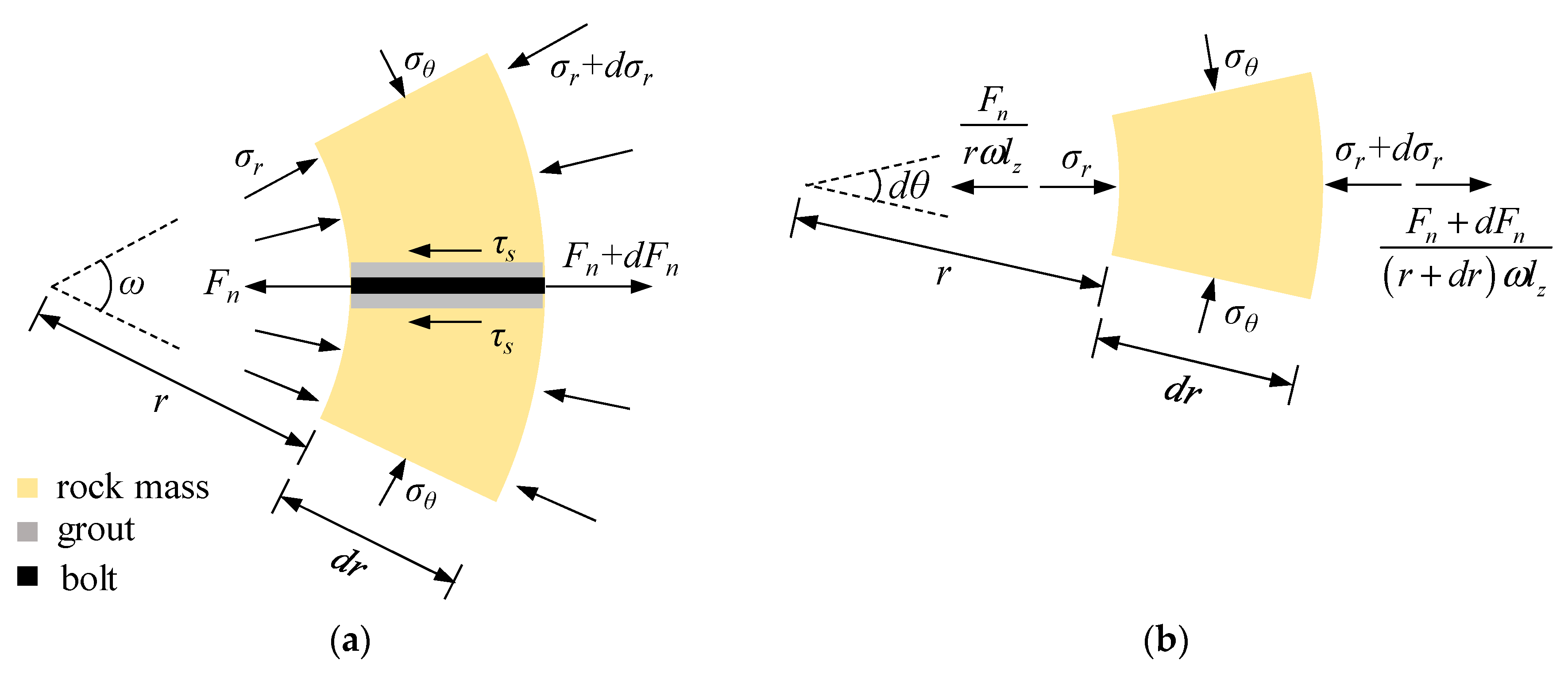
2.3. Equation of Equilibrium

For this axisymmetric problem, the equilibrium equation of the rock mass in an unbolted deep circular tunnel is:
d σ r d r = σ θ σ r r ,
where σr and σθ are the radial and tangential stresses, respectively.
As shown in Figure 2a, an infinitesimal element of the bolted rock mass is subjected to a radial stress σr, a tangential stress σθ, and a tension force in the bolt Fn. Supposing that the tension force can be spread uniformly around its tributary area lz, the equilibrium equation of an infinitesimal element of the bolted rock mass (Figure 2b) can be expressed as:
( σ r + d σ r ) ( r + d r ) d θ r σ r d θ 2 sin d θ 2 σ θ d r + d F n ω l z d θ = 0 .
Since the angle is infinitesimal, sin(/2) = /2. According to Figure 2a, the axial force in an infinitesimal bolt element dFn = πdsτsdr. Therefore, Equation (2) can be simplified to:
d σ r d r = σ θ σ r r + π d s τ s l z r ω ,
where τs is the shear stress at the bolt–rock interface and ds is the effective diameter of the bolts; see Section 2.7 for the determination of τs and ds.

2.4. Failure Criterions

2.4.1. Mohr–Coulomb Criterion

The Mohr–Coulomb criterion is expressed as:
σ θ = N σ r + Y ,
where N = (1 + sin φ)/(1 − sin φ) and Y = 2ccos φ/(1 − sin φ) are strength parameters; c and φ are the cohesion and friction angle of the rock mass, respectively; their corresponding peak values are Np, Yp, cp, and φp, respectively; and their corresponding residual values are Nr, Yr, cr, and φr, respectively.

2.4.2. Generalized Hoek–Brown Criterion

The generalized Hoek–Brown criterion [31] is expressed as:
σ θ = σ r + σ c i ( m b σ r σ c i + s ) a ,
where σci is the unconfined compressive strength of the intact rock, and mb, s, and a are semi-empirical parameters that characterize the rock mass. Their corresponding peak values are σci,p, mb,p, sp, and ap, respectively, and their corresponding residual values are σci,r, mb,r, sr, and ar, respectively.

2.5. Plastic Potential Equation

The Mohr–Coulomb criterion is chosen to be the plastic potential function, as follows:
g ( σ r , σ θ ) = σ θ K ψ σ r ,
where ψ is the dilatancy angle of the rock mass and Kψ = (1 + sin ψ)/(1 − sin ψ) is the dilatancy coefficient.

2.6. Equations of Strains and Displacements

For this axisymmetric problem, the radial strain εr and tangential strain εθ can be expressed in terms of the radial displacement ur:
ε r = d u r d r ,
ε θ = u r r .

2.6.1. In an Elastic Region

According to Hooke’s law, the elastic radial and tangential strains can be obtained using:
ε r e = 1 2 G [ ( 1 ν ) ( σ r p 0 ) ν ( σ θ p 0 ) ] ,
ε θ e = 1 2 G [ ( 1 ν ) ( σ θ p 0 ) ν ( σ r p 0 ) ] ,
where G = E/2/(1 + ν), E and ν are the shear modulus, Young′s modulus, and Poisson ratio of the rock mass, respectively.
Considering Equations (8) and (10) and the relation between the radial and tangential stresses in an elastic region—i.e., σθ + σr = 2p0—the radial displacement ur can be expressed as:
u r = 1 2 G ( p 0 σ r ) r .

2.6.2. In a Plastic Region

The radial and tangential strains are composed of the plastic strain components ( ε r p and ε θ p ) and the elastic strain components ( ε r e and ε θ e ), as follows:
ε r = ε r e + ε r p ,
ε θ = ε θ e + ε θ p .
Based on the plastic potential equation Equation (6), the plastic tangential strain and radial strain are formulated using the plastic multiplier λ:
ε r p = λ g ( σ r , σ θ ) σ r ,
ε θ p = λ g ( σ r , σ θ ) σ θ .
According to Equations (6), (14), and (15), the relation between the plastic tangential strain and the radial strain is:
ε r p = K ψ ε θ p .
By incorporating Equations (7)–(10) and Equations (12)–(16), the differential equation for the radial displacement ur is:
d u r d r + K ψ u r r = 1 2 G ( C 1 σ r + C 2 σ θ C 3 p 0 ) ,
where:
C 1 = 1 ν K ψ ν ,   C 2 = K ψ K ψ ν ν ,   C 3 = C 1 + C 2 .

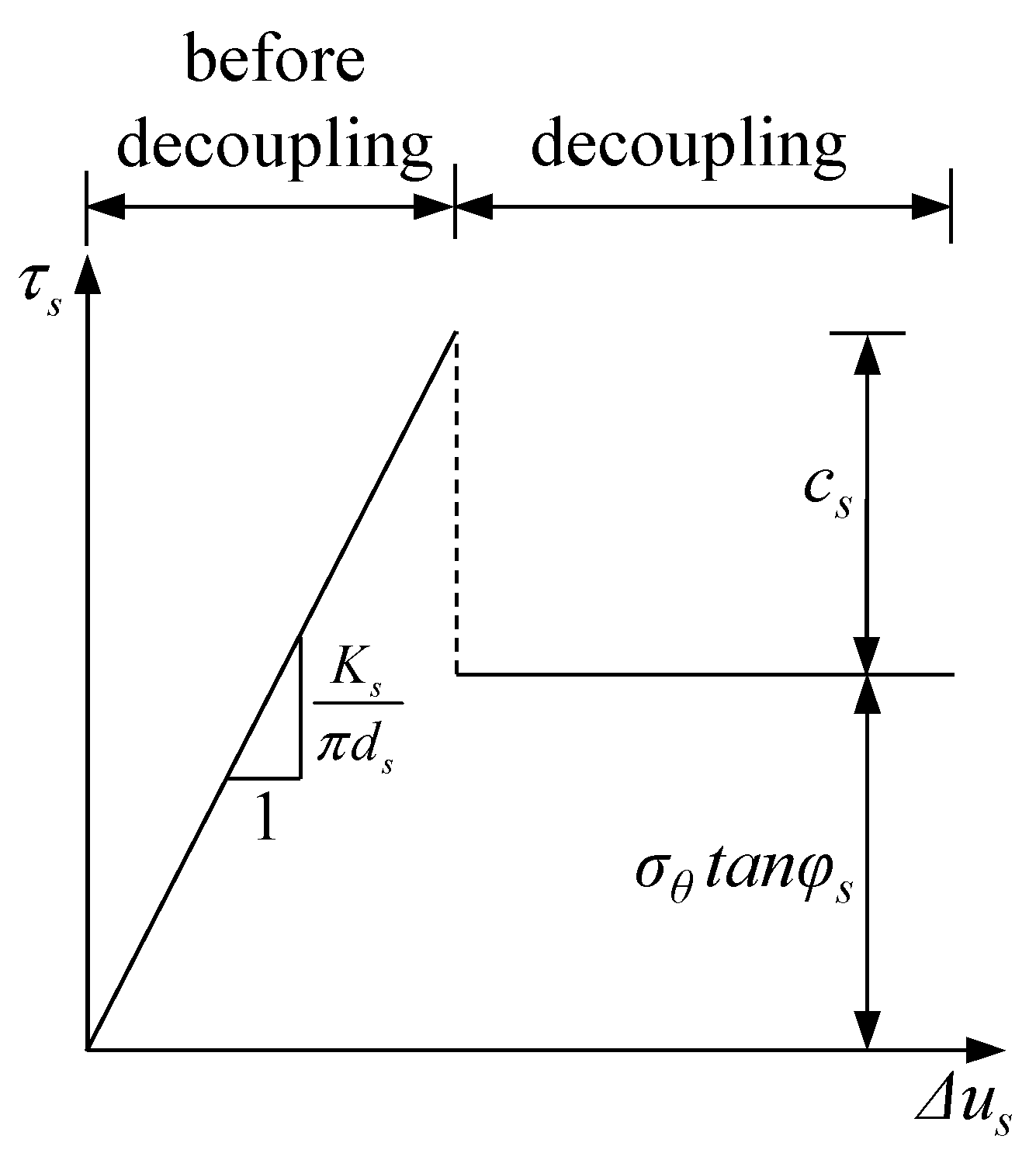
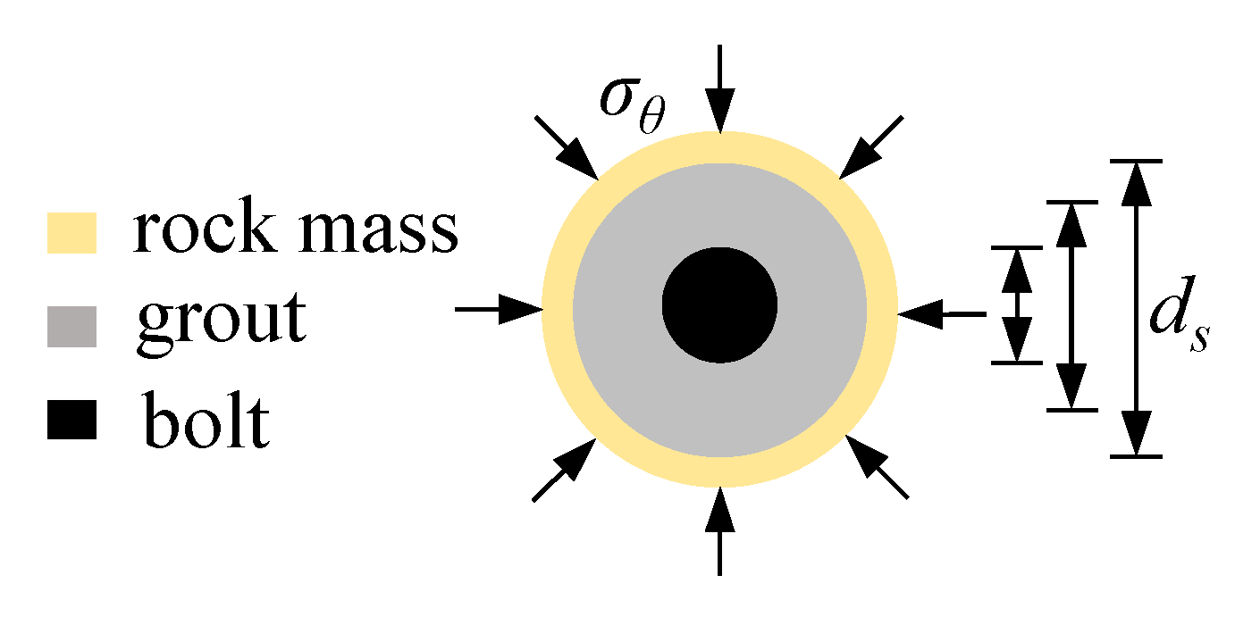
2.7. Interaction between the Rock Mass and the Passive Bolts

The pull-out tests show that the load–displacement curve is non-linear because of the decoupling at the bolt–rock interface and the confining pressure influences the shear strength of the interface greatly [32,33]. The spring–slider model [25] was employed here to characterize the relationship between the relative displacement Δus and shear stress τs at the bolt–rock interface, as shown in Figure 3.
The shear stress τs and tension force Fn of the bolt can be expressed as:
τ s = { K s Δ u s π d s , K s Δ u s π d s c s + σ θ tan φ s , σ θ tan φ s , K s Δ u s π d s > c s + σ θ tan φ s ,
F n = { 0 r = R + l b , R + l b r π d s τ s d r r < R + l b ,
where:
Δ u s = u r u r i n i u b r i g u b e l o ,   u b e l o = R + l b r F n E b A b d r .
Ks, cs, and φs are the shear stiffness, cohesion, and friction angle at the rock–bolt interface, respectively; Ab is the cross-sectional area of the bolt; u b r i g and u b e l o are the rigid displacement and the elongation of the bolt, respectively; ds is the effective diameter of the bolt, as shown in Figure 4, which may equal the diameter of the bolt, grout hole, or inside the grout because these interfaces are relatively weak in pull-out tests; and rb = R + lb is the radial distance from the far end of the bolt to the tunnel center. Note that Ks, ds, cs, and φs can be easily obtained from conventional pull-out tests [25].
As shown in Figure 5, the compression between the end plate and rock mass produces a tension force Fn(R) (Equation (20)) at the near end of the bolt and support pressure pep (Equation (21)) on the tunnel periphery. These two equations were used as boundary conditions in the calculation procedure (Appendix B):
F n ( R ) = K e p Δ u s ( R ) ,
p e p = F n ( R ) l z R ω ,
where Kep is the stiffness of the end plate, where Kep = 0 in the absence of the end plate.
Note that, compared with the original spring–slider model [25], the effects of the bolt elongation and the end plate were considered in this work.

3. Stress–Strain Analysis of the Rock Mass and Passive Bolts Using the Finite Difference Method

As shown in Figure 6, to simplify the analysis process, a bolted circular tunnel was divided into two parts: a bolted region and an unbolted region. The radial stress, tangential stress, and displacement at the bolted–unbolted interface are σr(R+lb), σθ(R+lb), and ur(R+lb), respectively.

3.1. Stress–Strain Analysis in an Unbolted Region

Notice that an unbolted region can be treated as an unbolted circular tunnel; therefore, stresses and displacements in an unbolted region can be obtained by replacing p and R in the equations in Appendix A with σr(R+lb) and R+lb, respectively.

3.2. Stress–Strain Analysis in a Bolted Region

In Figure 6, a bolted region is discretized into n annuluses with a uniform thickness Δr, starting from the bolted–unbolted interface. The ith annulus is bounded by two circles of r = ri−1 and r = ri. The radial stress σr(0), tangential stress σθ(0), and radial displacement ur(0) at the outer boundary of the bolted region (r = r(0) = R+lb) equal σr(R+lb), σθ(R+lb), and ur(R+lb), respectively. The number of the rock mass annuluses n and inner radius rj of each annulus can be respectively expressed as:
n = l b / Δ r ,
r ( i ) = r ( i 1 ) Δ r .
For the mechanical analysis of a bolted region, first, the elastoplastic state of the rock mass in the ith annulus is verified using Equation (4) (Mohr–Coulomb (M–C) rock mass) or Equation (5) (Hoek–Brown (H–B) rock mass); then, the stresses and displacements in an elastic annulus can be analyzed using the equations in Section 3.2.1; the stresses and displacements in a plastic annulus can be analyzed using the equations in Section 3.2.2; the behaviors of the passive bolts can be analyzed using the equations in Section 3.2.3; and the radius of the plastic region can be obtained in this process.

3.2.1. Stress–Strain Analysis in an Elastic Region

Considering Equation (3) and the relation between the radial and tangential stresses in an elastic region—i.e., σθ + σr = 2p0—the stresses at r = r(i) can be expressed in an incremental form by using the finite difference method, as follows:
σ r ( i ) = r ( i ) σ r ( i 1 ) + 2 Δ r p 0 + π d s Δ r τ s ( i 1 ) / ( l z ω ) r ( i ) + 2 Δ r ,
σ θ ( i ) = 2 p 0 σ r ( i ) .
According to Equation (11), the radial displacement at r = r(i) is:
u r ( i ) = 1 2 G ( p 0 σ r ( i ) ) r ( i ) .

3.2.2. Stress–Strain Analysis in a Plastic Region

By incorporating Equations (4) and (5) into Equation (3), the stresses at r = r(i) can be obtained. For the M–C rock mass, the stresses at r = r(i) are:
σ r ( i ) = r ( i ) σ r ( i 1 ) + Δ r Y r + π d s Δ r τ s ( i 1 ) / ( l z ω ) r ( i ) ( N r 1 ) Δ r ,
σ θ ( i ) = N r σ r ( i ) + Y r .
For the H–B rock mass, the stresses at r = r(i) are:
r ( i ) ( σ r ( i ) σ r ( i 1 ) ) = Δ r [ σ c i , r ( m b , r σ r ( i ) σ c i , r + s r ) a r + π d s τ s ( i 1 ) / ( l z ω ) ] ,
σ θ ( i ) = σ r ( i ) + σ c i , r ( m b σ r ( i ) σ c i , r + s r ) a r .
According to Equation (17), the radial displacement at r = r(j) is:
u r ( i ) = Δ r r ( i ) ( C 1 σ r ( i ) + C 2 σ θ ( i ) C 3 p 0 ) + 2 G r ( i ) u r ( i - 1 ) 2 G ( r ( i ) + K ψ Δ r ) .

3.2.3. Behaviors of the Passive Bolts

The shear stress at the bolt–rock interface (Equation (18)) and tension force in the bolts (Equation (19)) at r = r(i) can be respectively expressed as:
τ s ( j ) = { K s Δ u s ( i ) π d s , K s Δ u s ( i ) π d s c s + σ θ ( i ) tan φ s , σ θ ( i ) tan φ s , K s Δ u s ( i ) π d s > c s + σ θ ( i ) tan φ s ,
F n ( i ) = { 0 i = 0 , 0 i π d s τ s ( i ) Δ r i > 0 ,
where:
Δ u s ( i ) = u r ( i ) u r ( i ) i n i u r r i g u b ( i 1 ) e l o ,   u b ( i 1 ) e l o = 0 i 1 F n ( i 1 ) E b A b .
The initial radial displacement u r ( i ) i n i can be obtained by replacing p in the equations in Appendix A with βp0. Notice that, in Equations (20)–(31), once the contact radial stress σr(R+lb) and rigid displacement of the bolt u b r i g are inputted, the behavior of a bolted tunnel can be analyzed by repeating Equations (22)–(33) until i = n. Therefore, the key point of this solution is to determine the reasonable values of σr(R+lb) and u b r i g , where the details are listed in Appendix B.

4. Verification

The proposed solution was programmed using the MATLAB language (R2016a, MathWorks, Natick, MA, USA), and the verification is detailed in this section.

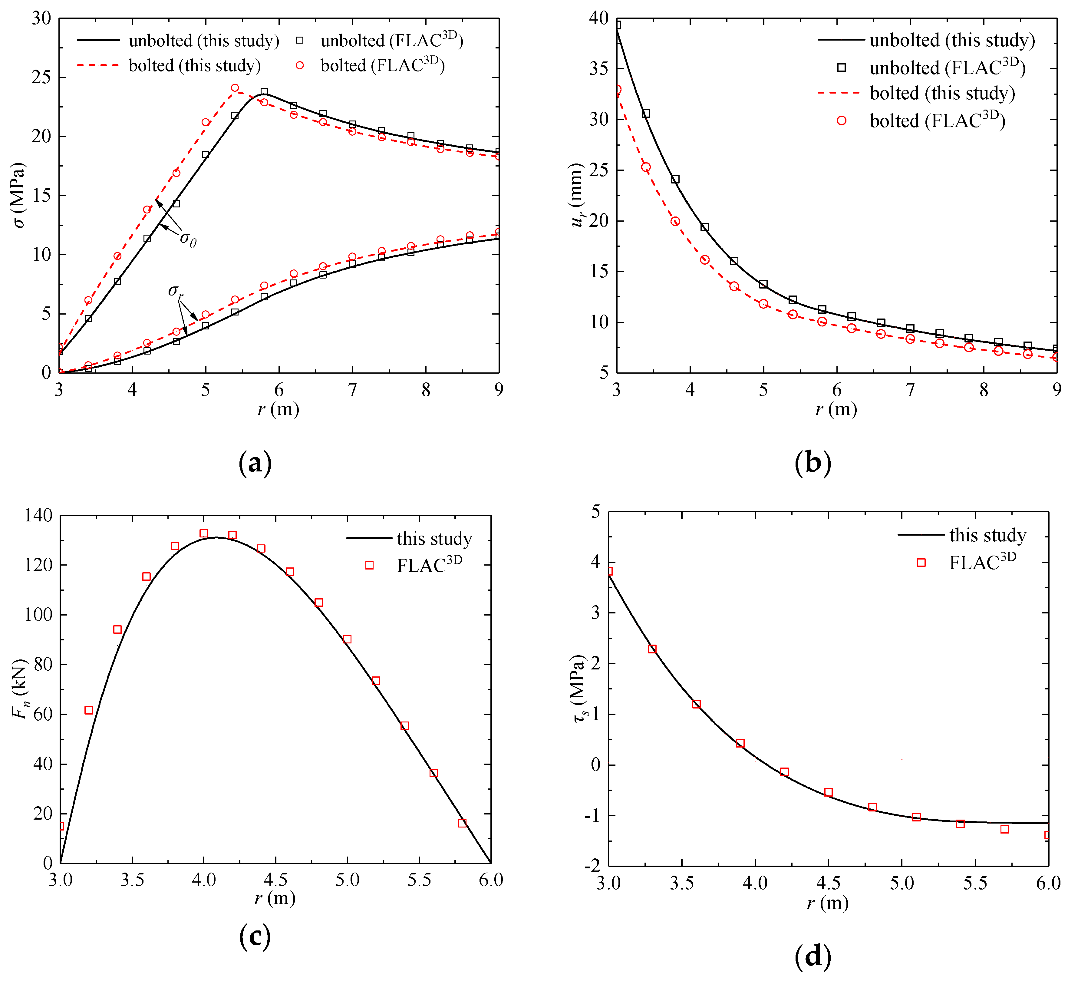
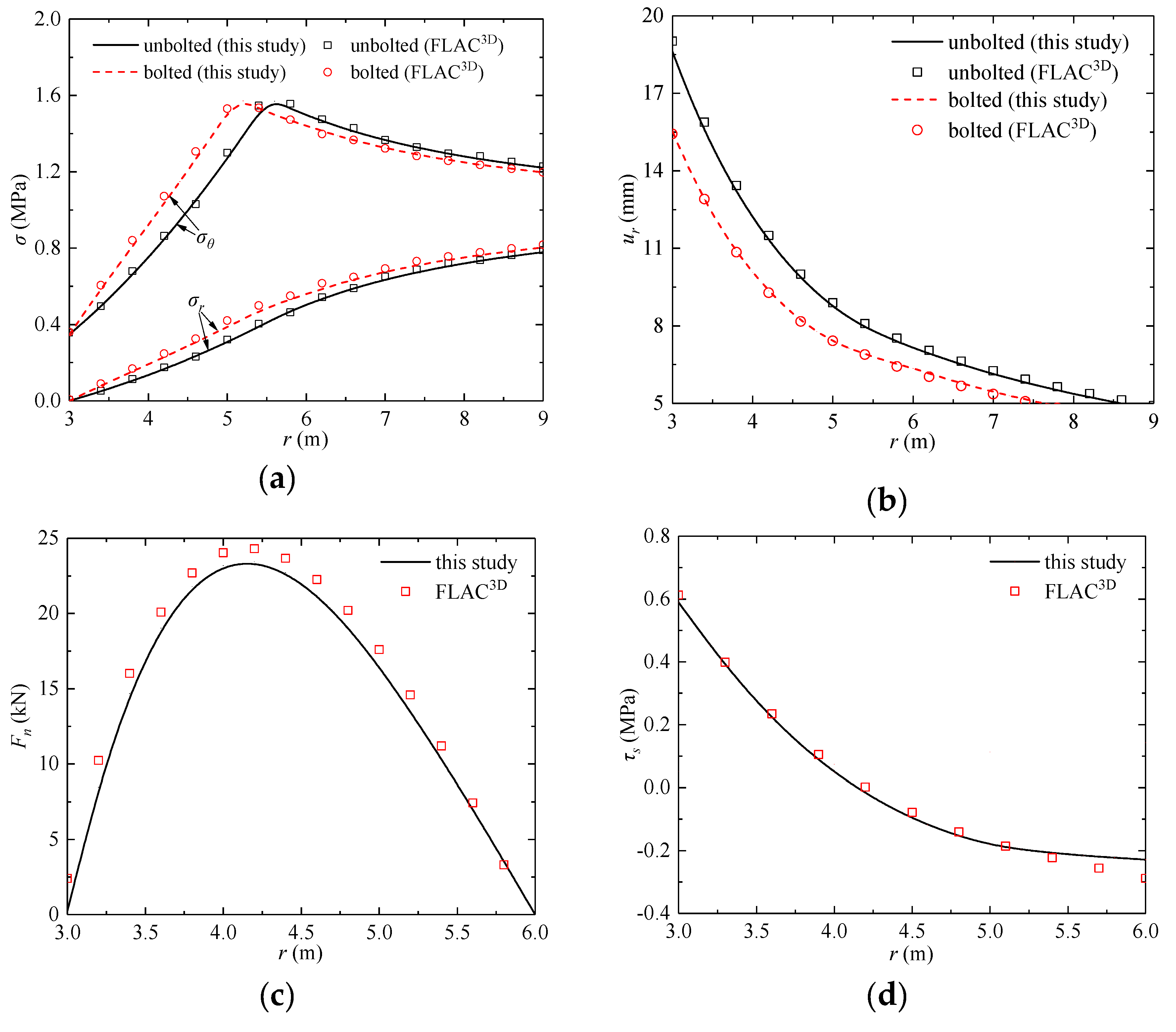
4.1. Comparison with the Results from the Commercial Numerical Software

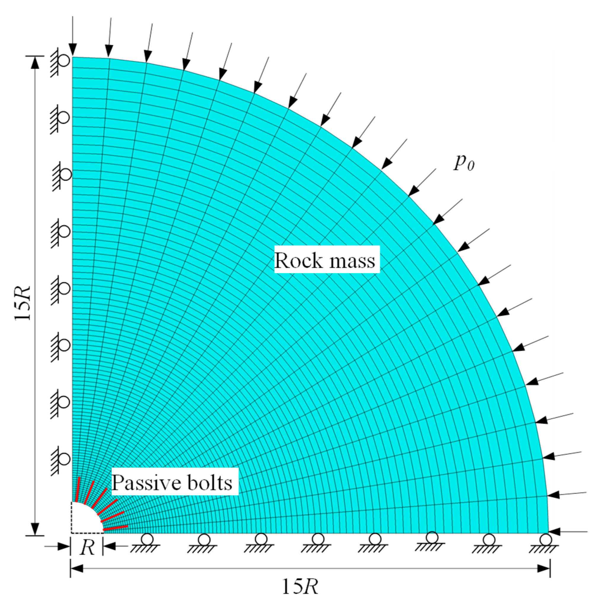
4.1.1. Establishment of the Numerical Model

The commercial numerical simulation software FLAC3D [34] was employed here to verify the accuracy of the proposed model. As shown in Figure 7, only a quarter of the circular tunnel was considered due to the symmetry of the problem. To simulate a deep tunnel under the hydrostatic and plane-strain condition, the outer boundary was 15R from the tunnel center, and its thickness was 1 m. Roller boundaries were set at the left and bottom boundaries, and the displacements in the tunnel axes directions were fixed. The hydrostatic stress field p0 was applied to the outer boundary. The passive bolts were installed uniformly around the tunnel, which was simulated using the cable element in FLAC3D.

4.1.2. Mohr–Coulomb Criterion

The properties employed in this section are listed in Table 1, and the parameters of the rock mass and passive bolts were adopted from the works conducted by Bobet and Einstein [2] and Cui et al. [29], respectively. As shown in Figure 8, the results calculated using the proposed model and the numerical model were in excellent agreement in both the bolted and unbolted cases. Figure 8a,b indicates that the passive bolts displayed a significant reinforcement effectiveness on the rock mass.

4.1.3. Generalized Hoek–Brown Criterion

The calculation parameters of the rock mass in Table 2 were taken from the work of Lee and Pietruszczak [35]. Except for Ks = 20 MPa, the properties of the passive bolts employed in this section were the same as in Table 1. The stresses and displacements of the rock mass, as well as the shear stress and tension force of the passive bolts obtained using the two methods, are plotted in Figure 9. It can be seen that the results of the proposed solution show good agreement with those from FLAC3D, and the reinforcement effectiveness of the passive bolts was significant.

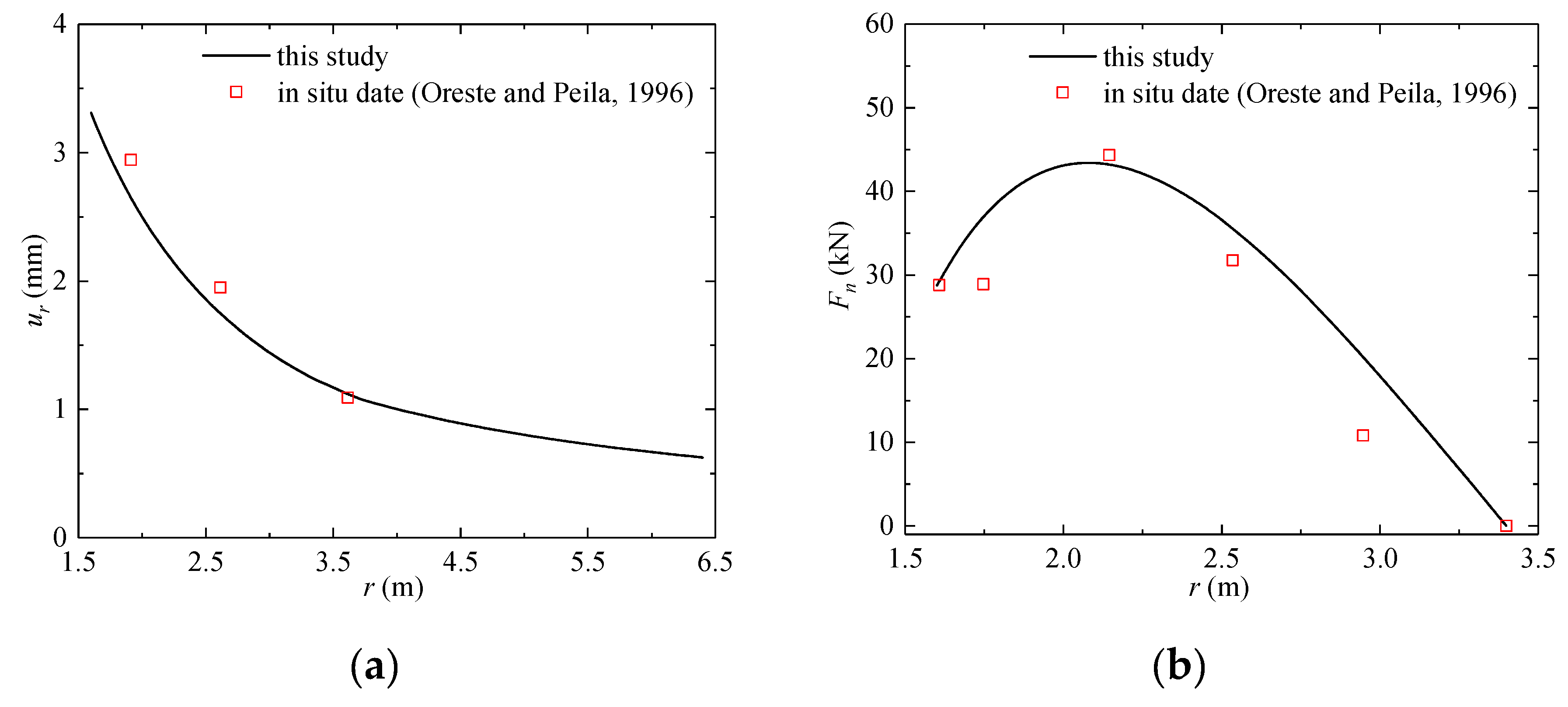
4.2. Comparison with the In Situ Test Results from the Kielder Experimental Tunnel

The results calculated using the proposed solution were compared with the measurements carried out in the Kielder experimental tunnel. The data were mainly from Oreste and Peila [8]. The rock mass in which the tests were carried out was a mudstone (RMR (Rock Mass Rating) = 32 and Q (Quantitative Classification of Rock Mass) = 0.33) with a strata thickness of 8 m. The main properties of the rock mass and passive bolts are listed in Table 3. The values of Ks and Kep were assumed to be 70 MPa and 30 MN/m, respectively. The tension force and radial displacement after 10 days from the initial bolt are potted in Figure 10. It can be observed that the calculation results agree well with the measured data.

5. Discussion

The following examples are given to explain the reinforcement effectiveness and mechanical behaviors of passive bolts. The generalized Hoek–Brown criterion was employed and the properties for a poor rock mass were adopted from the study conducted by Osgoui and Oreste [19], as shown in Table 4. The normalized displacement ur(R)/ u r ( R ) u b was employed to quantitatively evaluate the reinforcement effectiveness of the bolts, where ur(R) and u r ( R ) u b are the displacement at the tunnel periphery in the bolted and unbolted cases, respectively. Note that the smaller the normalized displacement, the better the reinforcement effectiveness.

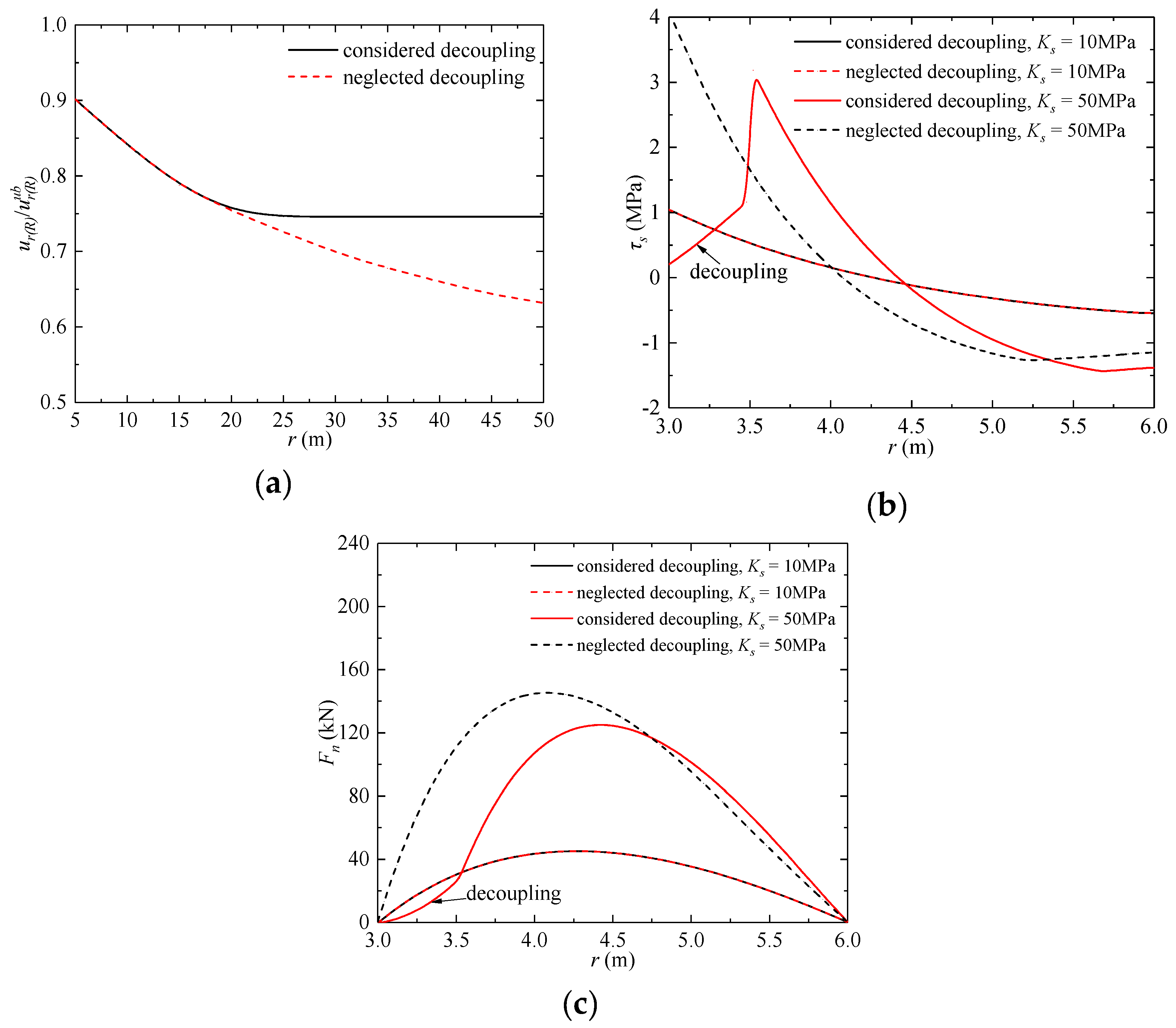
5.1. Comparison of the Solutions That Considered or Neglected Decoupling at the Bolt–Rock Interface

It was interesting to compare the results obtained from the models that considered and neglected the decoupling at the bolt–rock interface. Note that for the model that neglected the decoupling, the cohesion at the bolt–rock interface was fixed at ∞. The results plotted in Figure 11 show that the calculation results of the two models were identical before decoupling, and then the model that neglected the decoupling significantly overestimated the reinforcement effectiveness of the passive bolts, which may result in an unsafe design. Therefore, the decoupling at the bolt–rock interface should be considered in passive bolt designs.

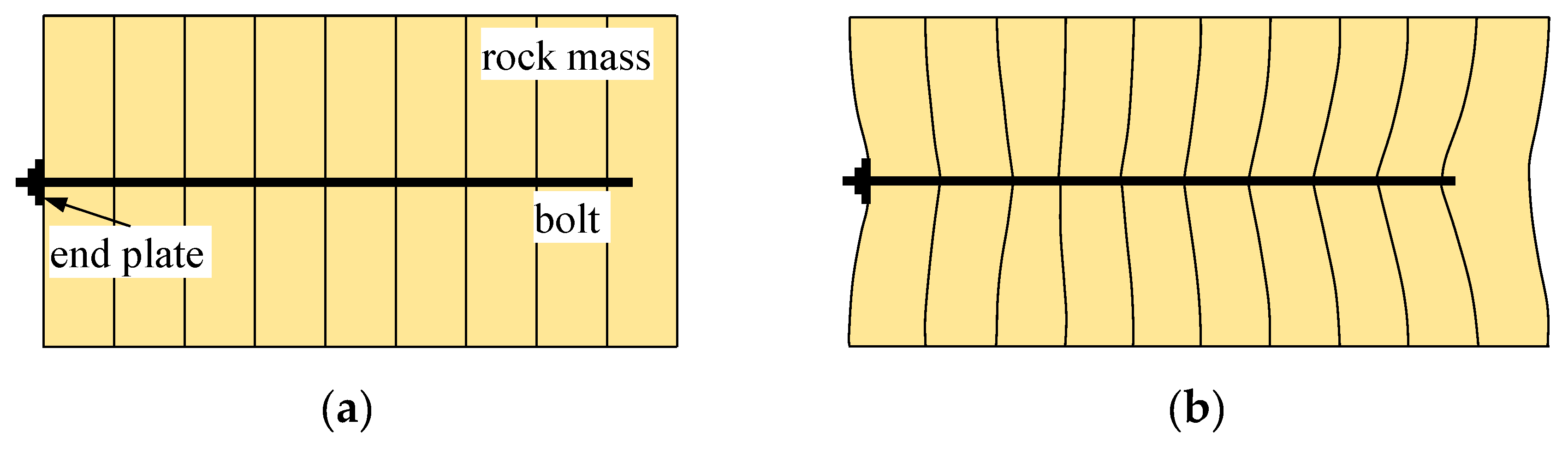
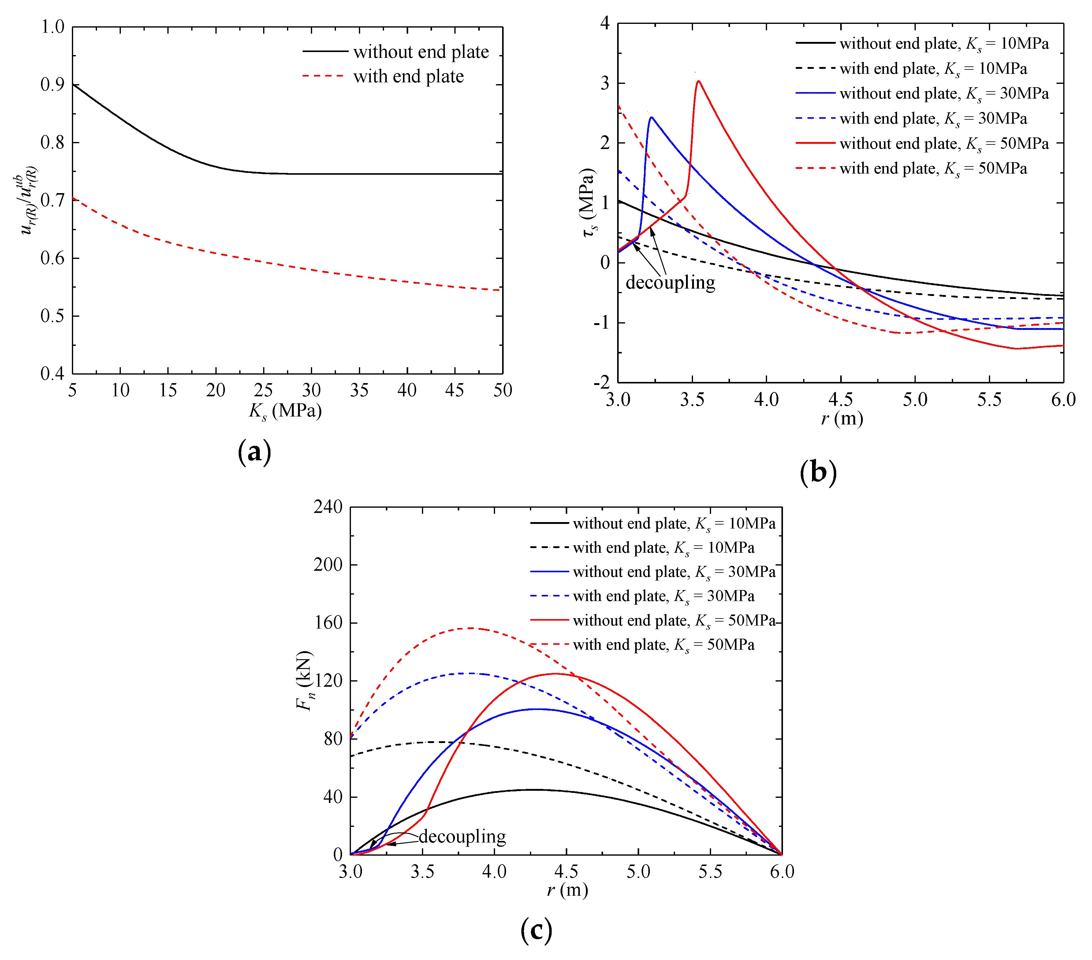
5.2. Effect of the End Plate and Shear Stiffness at the Bolt–Rock Interface

The results with different shear stiffnesses and with or without end plates are plotted in Figure 12. In the case without an end plate, Kep = 0 MN/m, while in the case with an end plate, Kep = 20 MN/m. As shown by the black solid line in Figure 12a, the normalized displacement decreased with the increasing shear stiffness before a critical value (about 20 MPa in this case), beyond which, the normalized displacement was almost constant because the shear stress at the bolt–rock interface increased with the increasing shear stiffness (see Figure 12b), while the decoupling at the bolt–rock interface occurred when the shear stress exceeds its capability. Moreover, Figure 12b shows that the maximum shear stress was generated at the end of bolts; therefore, the failure of the bolt–rock interface was more likely to start from the tunnel perimeter.
The red dashed line in Figure 12a illustrates that the end plate could effectively improve the reinforcement effectiveness of passive bolts by about 20% and avoids decoupling at the bolt–rock interface, which was due to the interaction between the end plate and rock mass exerting a support pressure on the tunnel periphery (see Figure 12c) and decreasing the shear stress (see Figure 12b). Figure 12c shows that the maximum tensile force in the case with an end plate was significantly larger than that in the other case, which implies that the tension failure of the bolts was more likely to occur in the case with an end plate.

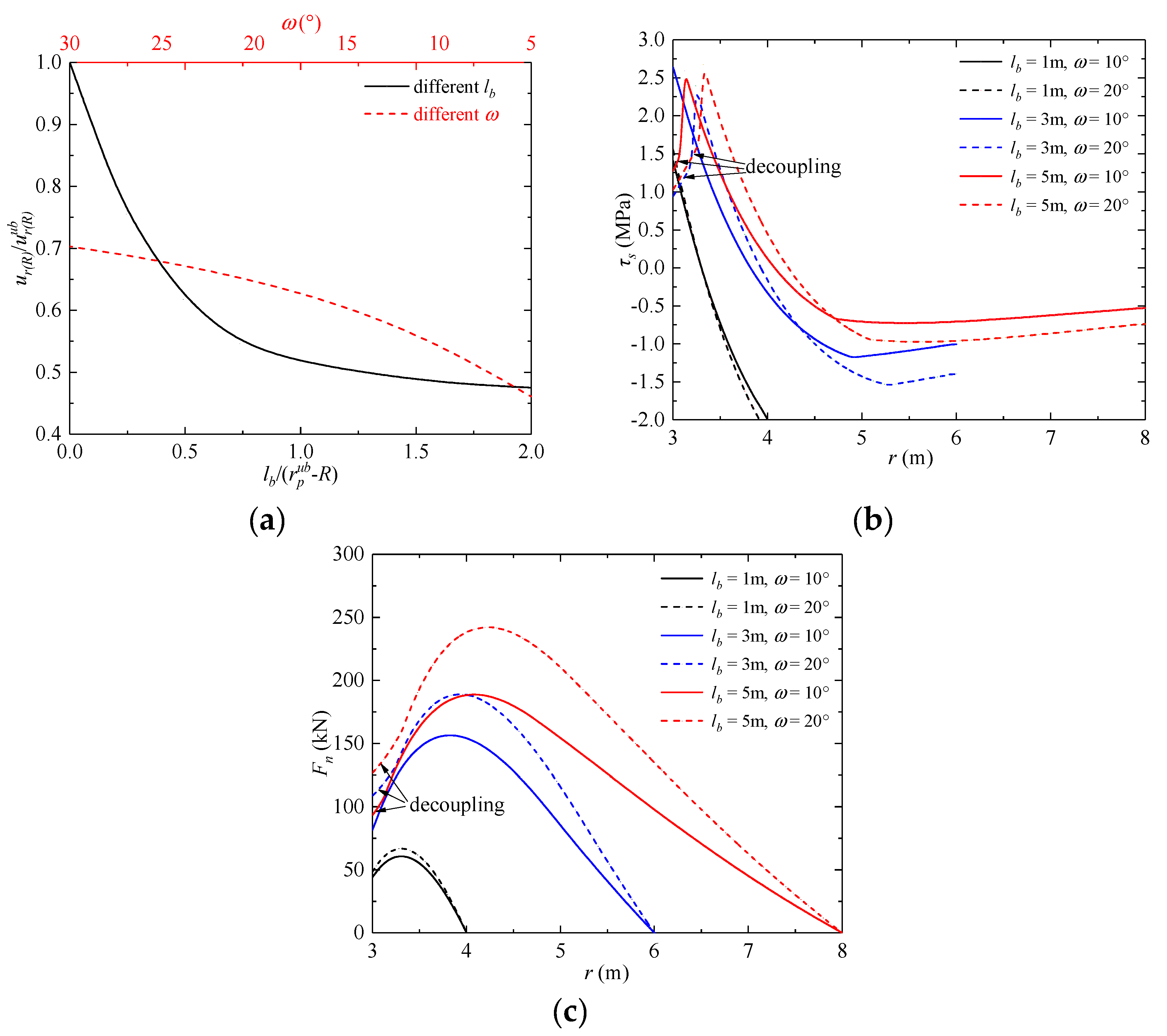
5.3. Effect of Bolt Length and Density

The normalized displacements with different bolt lengths and densities are plotted in Figure 13a, and the normalized bolt length lbn = lb/( r p u b R) [27] was taken as the abscissa, where r p u b is the plastic radius in the unbolted case. Note that if 0 ≤ lbn ≤ 1, the bolts were entirely embedded in the plastic region; when lbn > 1.0, the bolts penetrated the elastic region. Figure 13a shows that the normalized displacement decreased with the increasing normalized bolt length until lbn = 1.3, whereas the longer bolts could barely take more effective reinforcement. This phenomenon can be explained as follows: once the bolt section within the elastic region provided effective anchorage, the reinforcement effectiveness could not be further improved by increasing the bolt length. Therefore, the far end of the bolts should penetrate the elastic region to fully mobilize their effectiveness, while it was not necessary to over-extend the bolts beyond the range of the plastic region [25]. Furthermore, increasing the bolt density can result in better effectiveness (as shown by the red dashed line in Figure 13b).
Figure 13b,c plots the tension force and shear stress with different bolt lengths and densities. The figures show that the tension force and shear stress both increased with increasing bolt length and decreasing bolt density, while a large length or small density could cause the tension failure of the bolt and decoupling at the bolt–rock interface. Therefore, a reasonable length and density should be considered in passive bolt designs.

6. Conclusions

A new semi-analytical solution was established in this study for the mechanical analysis of fully grouted passive bolts and rock masses in tunnels. Comparisons and parameter analyses were conducted to assess the behavior of the proposed solution. The main conclusions are as follows:
(1) Comparisons with numerical results and in situ results indicate that the proposed solution could give a good estimation of the behaviors of passive bolts and rock masses in a deep circular tunnel.
(2) Compared with the model that considered the decoupling at the rock–bolt interface, a model that neglected the decoupling may significantly overestimate the reinforcement effectiveness of passive bolts, which may result in an unsafe design.
(3) The displacement of the rock mass decreased with increasing shear stiffness before a critical value, beyond which, decoupling at the bolt–rock interface occurred, resulting in the reduction of the reinforcement effectiveness.
(4) The interaction between the end plate and rock mass exerted a support pressure on the tunnel periphery and decreased the shear stress at the rock–bolt interface, thus effectively improving the reinforcement effectiveness and avoiding decoupling. The maximum tensile force in the bolts in the case with an end plate was significantly larger than that in the case without an end plate.
(5) To ensure the effectiveness and economy of passive bolts, the far end of the bolts should penetrate the elastic region, while it is not necessary to over-extend the bolts beyond the range of the plastic region. Increasing the bolt density can result in better effectiveness.
(6) The tension force and shear stress both increased with the increasing bolt length and decreasing bolt density, while a large length or small density may cause the tension failure of the bolt and decoupling at the bolt–rock interface.

Author Contributions

Conceptualization, M.W.; methodology, X.Z.; software, J.T.; validation, X.Z. and J.T.; formal analysis, W.Y.; investigation, X.Z.; resources, J.T.; data curation, J.T.; writing—original draft preparation, X.Z.; writing—review and editing, M.W.; visualization, Z.W.; supervision, D.L.; project administration, J.T.; funding acquisition, M.W. All authors have read and agreed to the published version of the manuscript.

Funding

This research was funded by National Natural Science Foundation of China, grant number No.51578458 and No.51878567 and No.51878568, and the China Railway Corporation Science and Technology Research and Development Program, grant number No.2017G007-H, No.2017G007-F and No.K2018G014.

Conflicts of Interest

The authors declare no conflict of interest.

Appendix A. Stress–Strain Analysis in an Unbolted Tunnel

As shown in Figure A1, when p < pcr, the rock mass behaves in an elastic–plastic manner, and a plastic region with radius rp and an elastic region are formed. When the support pressure is lower than a critical value pcr, a plastic region with radius rp will be formed.
Figure A1. An unbolted circular tunnel with a finite number of annuluses.
Applsci 10 04402 g0a1
For the M–C rock mass, pcr and rp can be obtained using [36]:
p c r = 2 p 0 Y p N p + 1 ,
r p = R [ p c r + Y r / ( N r 1 ) p + Y r / ( N r 1 ) ] 1 / ( N r 1 ) .
For the H–B rock mass, pcr and rp can be obtained using [37]:
2 ( p 0 p c r ) = σ c i , p ( m b , p p c r / σ c i , p + s p ) a p ,
r p = R exp [ ( m b , r p c r / σ c i , r + s r ) 1 a r ( m b , r p / σ c i , r + s r ) 1 a r ( 1 a r ) m b , r ] .
Equation (A3) can be solved numerically using the Newton–Raphson method.

Appendix A.1. Stress–Strain Analysis in an Unbolted Elastic Region

Resolving the differential equations composed using Equations (1) and (7)–(10) with the boundary condition σr = pcr at r = rp and σr = p0 at r = , the stresses and displacements in an elastic region (r > rp) can be calculated using Equations (A5)–(A7):
σ r = p 0 ( p 0 p c r ) r p 2 r 2 ,
σ θ = p 0 + ( p 0 p c r ) r p 2 r 2 ,
u r = 1 2 G ( p 0 p c r ) r p 2 r .
Note that when ppcr, the rock mass behaves elastically and its stresses and displacements can be calculated by replacing pcr and rp in Equations (A5)–(A7) with p and R, respectively.

Appendix A.2. Stress–Strain Analysis in an Unbolted Elastic Region

As shown in Figure A1, a plastic region is discretized into m annuluses with a uniform thickness Δr starting from the elastic–plastic interface. The jth annulus is bounded by two circles of r = rj−1 and r = rj. According to Equations (A5)–(A7), the stresses and displacement on the outer boundary of the plastic region (r = r(0) = rp) are:
σ r ( 0 ) = p c r ,
σ θ ( 0 ) = 2 p 0 p c r ,
u r ( 0 ) = 1 2 G ( p 0 p c r ) r p .
The number of the rock mass annuluses m and inner radius r(j) of each annulus can be expressed as:
m = ( r p R ) / Δ r ,
r ( j ) = r ( j 1 ) Δ r .
Incorporating Equations (4) and (5) into Equation (1), the stresses at r = r(j) can be obtained. For the M–C rock mass, the stresses at r = r(j) can be expressed in an incremental form by using the finite difference method, as follows:
σ r ( j ) = r ( j ) σ r ( j 1 ) + Δ r Y r r ( j ) ( N r 1 ) Δ r ,
σ θ ( j ) = N r σ r ( j ) + Y r .
For the H–B rock mass, the stresses at r = r(j) are:
r ( j ) ( σ r ( j ) σ r ( j 1 ) ) = Δ r σ c i , r ( m b , r σ r ( j ) σ c i , r + s r ) a r ,
σ θ ( j ) = σ r ( j ) + σ c i , r ( m b σ r ( j ) σ c i , r + s r ) a r .
Incorporating Equations (4) and (5) into Equation (17), the radial displacement at r = r(i) is:
u r ( i ) = Δ r r ( j ) ( C 1 σ r ( j ) + C 2 σ θ ( j ) C 3 p 0 ) + 2 G r ( j ) u r ( j - 1 ) 2 G ( r ( j ) + K ψ Δ r ) .
Equation (A15) can be solved numerically using the Newton–Raphson method. By repeating Equations (A8)–(A17) until j = m, the stresses and displacements in a plastic region can be obtained.

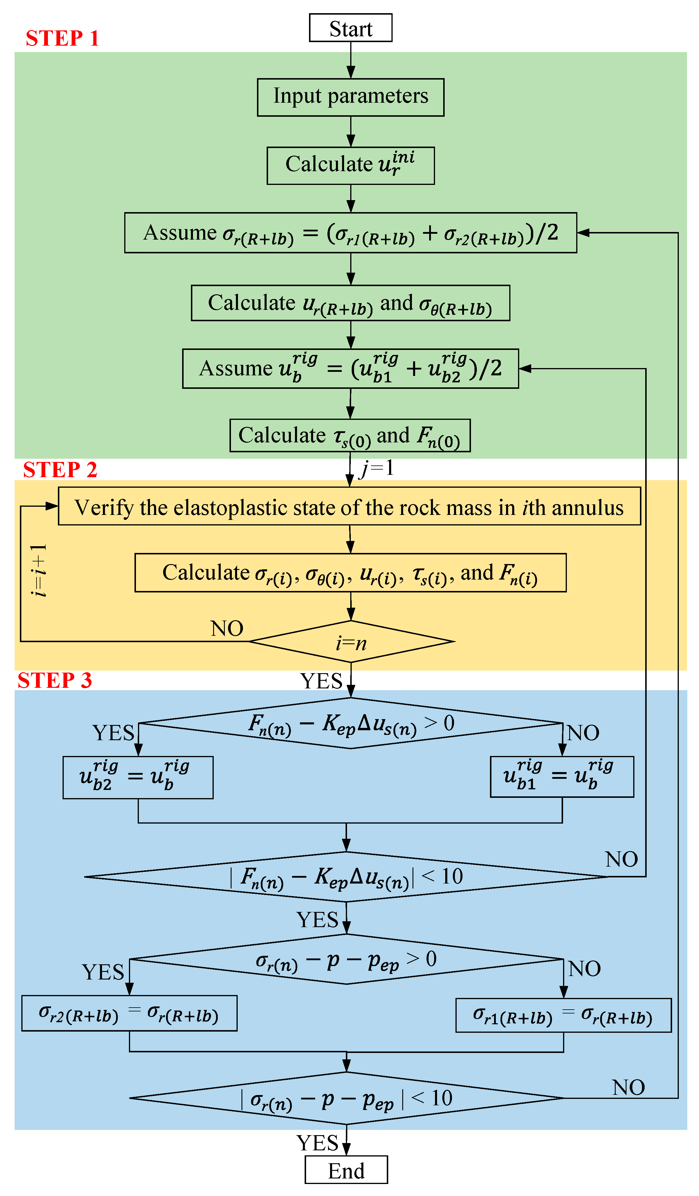
Appendix B. Calculation Procedure

It is obvious that the contact radial stress is greater than zero and smaller than p0; i.e., 0 < σr(R+lb) < p0. The rigid displacement along the whole bolt is greater than zero and smaller than a large value (such as 10 m), i.e., 0 < u b r i g < 10. The reasonable values of σr(R+lb) and u b r i g can be obtained using two boundary conditions in combination with the bisection method, and the details are described below and plotted in Figure A2.
Step 1. Preliminary calculations
(1)
Input parameters: R, p0, β, p, E, μ, ψ, Eb, lb, ds, Ab, lz, ω, Ks, Kep, cs, φs, Δr, cp, cr, φp, φr, σci,p, σci,r, mb,p, mb,r, sp, sr, ap, and ar.
(2)
Calculate u r i n i by replacing p in the equations in Appendix A with βp0.
(3)
Assume an initial value of σr(R+lb) = (σr1(R+lb)+σr2(R+lb))/2, where σr1(R+lb) = 0 and σr2(R+lb) = p0.
(4)
Calculate ur(R+lb) and σθ(R+lb) by replacing p and R in the equations in Appendix A with σr(R+lb) and R+lb, respectively.
(5)
Assume an initial value of u b r i g = ( u b 1 r i g + u b 2 r i g )/2, where u b 1 r i g = 0 and u b 2 r i g = 10.
(6)
Calculate τs(0) and Fn(0) using Equations (32) and (33), respectively.
Step 2. The sequence of calculation for each annulus in a bolted region
(1)
Verify the elastoplastic state of the rock mass in the ith annulus using Equation (4) (M–C rock mass) or Equation (5) (H–B rock mass).
(2)
Calculate σr(i) using Equation (24) (elastic state), or Equation (27) (plastic state, M–C rock mass) or Equation (29) (plastic state, H–B rock mass).
(3)
Calculate σθ(i) using Equation (25) (elastic state), or Equation (28) (plastic state, M–C rock mass) or Equation (30) (plastic state, H–B rock mass).
(4)
Calculate ur(i) using Equation (26) (elastic state) or Equation (31) (plastic state).
(5)
Calculate τb(i) and Fn(i) using Equations (32) and (33), respectively.
Repeat (1)–(5) until i = n.
Step 3. Verify the boundary conditions
(1) Verify the boundary condition at the near end of the bolt (Equation (A18)). If this condition is satisfied, verify the next boundary condition; otherwise, the bisection method is employed to determine another u b r i g until Equation (A18) is satisfied:
F n ( n ) = K e p Δ u s ( n ) .
(2) Verify the boundary condition at the tunnel periphery (Equation (A19)). If this condition is satisfied, the values of u b r i g and σr(R+lb) are reasonable; otherwise, the bisection method is employed to determine another σr(R+lb) until Equation (A19) is satisfied:
σ r ( n ) = p e p + p = K e p Δ u s ( n ) l z R ω + p .
Figure A2. Calculation procedure of the proposed solution.
Applsci 10 04402 g0a2

References

  1. Kovári, K. History of the sprayed concrete lining method—Part I: Milestones up to the 1960s. Tunn. Undergr. Space Technol. 2003, 18, 57–69. [Google Scholar] [CrossRef]
  2. Bobet, A.; Einstein, H. Tunnel reinforcement with rockbolts. Tunn. Undergr. Space Technol. 2011, 26, 100–123. [Google Scholar] [CrossRef]
  3. Li, P.F.; Wang, F.; Fang, Q. Undrained analysis of ground reaction curves for deep tunnels in saturated ground considering the effect of ground reinforcement. Tunn. Undergr. Space Technol. 2018, 71, 579–590. [Google Scholar] [CrossRef]
  4. Bobet, A. Elastic solution for deep tunnels. Application to excavation damage zone and rockbolt support. Rock Mech. Rock Eng. 2009, 42, 147–174. [Google Scholar] [CrossRef]
  5. Carranza-Torres, C. Analytical and numerical study of the mechanics of rockbolt reinforcement around tunnels in rock masses. Rock Mech. Rock Eng. 2009, 42, 175–228. [Google Scholar] [CrossRef]
  6. Fahimifar, A.; Ranjbarnia, M. Analytical approach for the design of active grouted rockbolts in tunnel stability based on convergence-confinement method. Tunn. Undergr. Space Technol. 2009, 24, 363–375. [Google Scholar] [CrossRef]
  7. Fahimifar, A.; Soroush, H. A theoretical approach for analysis of the interaction between grouted rockbolts and rock masses. Tunn. Undergr. Space Technol. 2005, 20, 333–343. [Google Scholar] [CrossRef]
  8. Oreste, P.; Peila, D. Radial passive rockbolting in tunnelling design with a new convergence-confinement model. In International Journal of Rock Mechanics and Mining Sciences & Geomechanics Abstracts; Elsevier: Amsterdam, The Netherlands, 1996; pp. 443–454. [Google Scholar]
  9. Stille, H.; Holmberg, M.; Nord, G. Support of weak rock with grouted bolts and shotcrete. In International Journal of Rock Mechanics and Mining Sciences & Geomechanics Abstracts; Elsevier: Amsterdam, The Netherlands, 1989; pp. 99–113. [Google Scholar]
  10. Zou, J.; Chen, K.; Pan, Q. An improved numerical approach in surrounding rock incorporating rockbolt effectiveness and seepage force. Acta Geotech. 2018, 13, 707–727. [Google Scholar] [CrossRef]
  11. Wang, G.; Liu, C.; Jiang, Y.; Wu, X.; Wang, S. Rheological model of DMFC rockbolt and rock mass in a circular tunnel. Rock Mech. Rock Eng. 2015, 48, 2319–2357. [Google Scholar] [CrossRef]
  12. Wang, G.; Han, W.; Jiang, Y.; Luan, H.; Wang, K. Coupling analysis for rock mass supported with CMC or CFC rockbolts based on viscoelastic method. Rock Mech. Rock Eng. 2019, 52, 4565–4588. [Google Scholar] [CrossRef]
  13. Zou, J.F.; Xia, Z.Q.; Dan, H.C. Theoretical solutions for displacement and stress of a circular opening reinforced by grouted rock bolt. Geomech. Eng. 2016, 11, 439–455. [Google Scholar] [CrossRef]
  14. Freeman, T. The behaviour of fully-bonded rock bolts in the Kielder experimental tunnel. Tunn. Tunn. Int. 1978, 10, 37–40. [Google Scholar]
  15. Cui, L.; Dong, Y.-K.; Sheng, Q.; Shen, Q. New numerical procedures for fully-grouted bolt in the rock mass with slip and non-slip cases at the rock-bolt interface. Constr. Build. Mater. 2019, 204, 849–863. [Google Scholar] [CrossRef]
  16. Indraratna, B.; Kaiser, P. Analytical model for the design of grouted rock bolts. Int. J. Numer. Anal. Methods Geomech. 1990, 14, 227–251. [Google Scholar] [CrossRef]
  17. Indraratna, B.; Kaiser, P. Design for grouted rock bolts based on the convergence control method. In International Journal of Rock Mechanics and Mining Sciences & Geomechanics Abstracts; Elsevier: Amsterdam, The Netherlands, 1990; pp. 269–281. [Google Scholar]
  18. Osgoui, R.R.; Oreste, P. Convergence-control approach for rock tunnels reinforced by grouted bolts, using the homogenization concept. Geotech. Geol. Eng. 2007, 25, 431–440. [Google Scholar] [CrossRef]
  19. Osgoui, R.R.; Oreste, P. Elasto-plastic analytical model for the design of grouted bolts in a Hoek–Brown medium. Int. J. Numer. Anal. Methods Geomech. 2010, 34, 1651–1686. [Google Scholar] [CrossRef]
  20. Osgoui, R.R.; Ünal, E. An empirical method for design of grouted bolts in rock tunnels based on the Geological Strength Index (GSI). Eng. Geol. 2009, 107, 154–166. [Google Scholar] [CrossRef]
  21. Yu, T.Z.; Xian, C.J. Behaviour of rock bolting as tunnelling support. In Proceedings of the International Symposium on Rock Bolting; Abisko: Abisko, Sweden, 1983; pp. 87–92. [Google Scholar]
  22. Cai, Y.; Esaki, T.; Jiang, Y. A rock bolt and rock mass interaction model. Int. J. Rock Mech. Min. Sci. 2004, 41, 1055–1067. [Google Scholar] [CrossRef]
  23. Cai, Y.; Esaki, T.; Jiang, Y. An analytical model to predict axial load in grouted rock bolt for soft rock tunnelling. Tunn. Undergr. Space Technol. 2004, 19, 607–618. [Google Scholar] [CrossRef]
  24. Li, C.; Stillborg, B. Analytical models for rock bolts. Int. J. Rock Mech. Min. Sci. 1999, 36, 1013–1029. [Google Scholar] [CrossRef]
  25. Guan, Z.; Jiang, Y.; Tanabasi, Y.; Huang, H. Reinforcement mechanics of passive bolts in conventional tunnelling. Int. J. Rock Mech. Min. Sci. 2007, 44, 625–636. [Google Scholar] [CrossRef]
  26. Oreste, P. Distinct analysis of fully grouted bolts around a circular tunnel considering the congruence of displacements between the bar and the rock. Int. J. Rock Mech. Min. Sci. 2008, 45, 1052–1067. [Google Scholar] [CrossRef]
  27. Tan, C.H. Difference solution of passive bolts reinforcement around a circular opening in elastoplastic rock mass. Int. J. Rock Mech. Min. Sci. 2016, 81, 28–38. [Google Scholar] [CrossRef]
  28. Tan, C.H. Passive bolts reinforcement around a circular opening in strain-softening elastoplastic rock mass. Int. J. Rock Mech. Min. Sci. 2016, 88, 221–234. [Google Scholar] [CrossRef]
  29. Cui, L.; Zheng, J.-J.; Sheng, Q.; Pan, Y. A simplified procedure for the interaction between fully-grouted bolts and rock mass for circular tunnels. Comput. Geotech. 2019, 106, 177–192. [Google Scholar] [CrossRef]
  30. Möller, S.C. Tunnel Induced Settlements and Structural Forces in Linings; Univ. Stuttgart, Inst. f. Geotechnik: Stuttgart, Germany, 2006. [Google Scholar]
  31. Hoek, E.; Carranza-Torres, C.; Corkum, B. Hoek-Brown failure criterion-2002 edition. Proc. Narms-Tac. 2002, 1, 267–273. [Google Scholar]
  32. Jafari, A. A Laboratory Study of Bond Failure Mechanism in Deformed Rock Bolts Using a Modified Hoek Cell. In Proceedings of the Frontiers of Rock Mechanics & Sustainable Development in the Century—Isrm International Symposium-asian Rock Mechanics Symposium, Beijing, China, 11–14 September 2001. [Google Scholar]
  33. Malvar, L.J. Bond of Reinforcement Under Controlled Confinement. Aci. Mater. J. 1991, 89, 47. [Google Scholar]
  34. Itasca. FLAC3D V5. 0, Fast Lagrangian Analysis of Continua in 3 Dimensions; User’s Guide; Itasca Consulting Group: Minneapolis, MN, USA, 2011. [Google Scholar]
  35. Lee, Y.-K.; Pietruszczak, S. A new numerical procedure for elasto-plastic analysis of a circular opening excavated in a strain-softening rock mass. Tunn. Undergr. Space Technol. 2008, 23, 588–599. [Google Scholar] [CrossRef]
  36. Brady, B.H.; Brown, E.T. Rock Mechanics: For Underground Mining: Springer Science & Business Media; Springer: New York, NY, USA, 1993. [Google Scholar]
  37. Sharan, S. Analytical solutions for stresses and displacements around a circular opening in a generalized Hoek–Brown rock. Int. J. Rock Mech. Min. Sci. 2008, 1, 78–85. [Google Scholar] [CrossRef]
Figure 1. A deep circular tunnel reinforced with passive bolts: (a) the cross-section and (b) the longitudinal section.
Applsci 10 04402 g001
Figure 2. Static equilibrium condition for an infinitesimal element of the bolted rock mass: (a) stresses in the rock mass and bolt tension and (b) equivalent stresses.
Applsci 10 04402 g002
Figure 3. The spring–slider model of the bolt–rock interface.
Applsci 10 04402 g003
Figure 4. The effective diameter of the bolt.
Applsci 10 04402 g004
Figure 5. Schematic representation of the interaction between the rock mass and the end plate: (a) undeformed rock mass and (b) deformed rock mass.
Applsci 10 04402 g005
Figure 6. A bolted circular tunnel with a finite number of annuluses.
Applsci 10 04402 g006
Figure 7. Schematic representation of the numerical model.
Applsci 10 04402 g007
Figure 8. Comparison of the results calculated using the proposed model and numerical model (Mohr–Coulomb (M–C) rock mass): (a) σr and σθ, (b) ur, (c) Fn, and (d) τs.
Applsci 10 04402 g008
Figure 9. Comparison of the results calculated using the proposed model and numerical model (Hoek–Brown (H–B) rock mass): (a) σr and σθ, (b) ur, (c) Fn, and (d) τs.
Applsci 10 04402 g009
Figure 10. Comparison of the calculation results and the measured data: (a) ur and (b) Fn.
Applsci 10 04402 g010
Figure 11. The results obtained from the models that considered or neglected decoupling: (a) ur(R)/ u r ( R ) u b , (b) τs, and (c) Fn (Eb = 210 GPa, ds = 25 mm, Ab = 491 mm2, lz = 1 m, lb = 3 m, ω = 10°, Kep = 0 MN/m, β = 0.3, p = 0, cg = 1 MPa, φg = 40°).
Applsci 10 04402 g011
Figure 12. The calculation results with different shear stiffnesses and with or without an end plate: (a) ur(R)/ u r ( R ) u b , (b) τs, and (c) Fn (Eb = 210 GPa, ds = 25 mm, Ab = 491 mm2, lz = 1 m, lb = 3 m, ω = 10°, β = 0.3, p = 0, cg = 1 MPa, φg = 40°).
Applsci 10 04402 g012
Figure 13. The calculation results with different bolt lengths and densities: (a) lbn, (b) τs, and (c) Fn (Eb = 210 GPa, ds = 25 mm, Ab = 491 mm2, lz = 1 m, lb = 3 m, ω = 10°, Ks = 50 MPa, Kep = 20 MN/m, β = 0.3, p = 0, cg = 1 MPa, φg = 40°).
Applsci 10 04402 g013
Table 1. The parameters of rock mass and passive bolts [2,29].
Rock MassPassive Bolts
Symbol (Unit)ValueSymbol (Unit)Value
R (m)3Eb (GPa)210
p0 (MPa)1lb (m)3
E (GPa)0.5ds (mm)25
μ0.2Ab (mm2)491
cp (MPa)0.1lz (m)1
cr (MPa)0.1ω (°)10
φp (°)30Ks (MPa)10
φr (°)30Kep (MN/m)0
ψ (°)0β0.3
p (MPa)0
cs (kPa)
φs (°)0
Table 2. The parameters of rock mass [35].
Symbol (Unit)ValueSymbol (Unit)Value
R (m)3mb,r2
p0 (MPa)15sp4 × 10−3
E (GPa)5.7sr4 × 10−3
μ0.25ap0.55
σci,p (MPa)30ar0.55
σci,r (MPa)30ψ (°)15
mb,p2
Table 3. The parameters of rock mass and passive bolts [8].
Rock MassPassive Bolts
Symbol (Unit)ValueSymbol (Unit)Value
R (m)1.6Eb (GPa)210
p0 (MPa)2.6lb (m)1.8
E (GPa)5ds (mm)25
μ0.25Ab (mm2)491
σci,p (MPa)37lz (m)0.9
σci,r (MPa)37ω (°)32
mb,p0.1Ks (MPa)70
mb,r0.05Kep (MN/m)30
sp8 × 10−5β0.3
sr1 × 10−5p (MPa)0
ap0.5cs (kPa)
ar0.5φs (°)0
ψ (°)0
Table 4. The parameters of the rock mass [19].
Symbol (Unit)ValueSymbol (Unit)Value
R (m)3mb,r0.615
p0 (MPa)5sp7.3 × 10−4
E (GPa)2.57sr1.7 × 10−4
μ0.25ap0.516
σci,p (MPa)30ar0.538
σci,r (MPa)24ψ (°)0
mb,p0.981

