Retinex Based Image Enhancement via General Dictionary Convolutional Sparse Coding

Abstract

Retinex theory represents the human visual system by showing the relative reflectance of an object under various illumination conditions. A feature of this human visual system is color constancy, and the Retinex theory is designed in consideration of this feature. The Retinex algorithms have been popularly used to effectively decompose the illumination and reflectance of an object. The main aim of this paper is to study image enhancement using convolution sparse coding and sparse representations of the reflectance component in the Retinex model over a learned dictionary. To realize this, we use the convolutional sparse coding model to represent the reflectance component in detail. In addition, we propose that the reflectance component can be reconstructed using a trained general dictionary by using convolutional sparse coding from a large dataset. We use singular value decomposition in limited memory to construct a best reflectance dictionary. This allows the reflectance component to provide improved visual quality over conventional methods, as shown in the experimental results. Consequently, we can reduce the difference in perception between humans and machines through the proposed Retinex-based image enhancement.

1. Introduction

The color of an object determined by a machine visual system (MVS) such as a digital camera is based on the amount of light reflected from it. On the other hand, the human visual system (HVS) determines the color of an object by considering the details of the surrounding environment and changes in overall illumination [1]. The complex HVS automatically recognizes the changes in illumination and easily recognizes the original color of the object. This feature of the HVS is called color constancy and has been studied for a long time [2,3]. Owing to the inconsistency between the HVS and the MVS under various illumination conditions, a machine cannot obtain the same image as a human. These inconsistencies also cause algorithmic errors in functions such as color separation, pattern recognition and object tracking. Therefore, to improve the performance of MVS, it is important to understand the color constancy of HVS.

The Retinex concept by Land and McCann [4,5,6,7] combines the functions of retina and cortex, and explains how the HVS perceives color. If S is defined as the value of an image in the spatial domain $\mathsf{\Omega }$, the image value in the Retinex model mainly depends on two factors: the amount of illumination projected onto the object in the image and the amount of illumination reflected by the object in the image. Based on these two components, S can be constructed with the reflectance function R and illumination function L [8] as follows:

$$S\left(x\right)=R\left(x\right)·L\left(x\right)$$

(1)

where, $0<R<1$ (reflectivity) and $0<L<\infty$ (illumination effect), $\forall x\in \mathsf{\Omega }$

The HVS can recognize both the illumination component and the reflectance component, and is able to remove the illumination component. This is called color constancy. Therefore, the HVS can recognize the constant color of an object, while ignoring the changing illumination. Removing the illumination component from the image can cause dark areas in the low-light image enhancement application to represent the original color of the object, which can increase the success rate of other algorithms on the machine. Also, it is possible to improve the edge, texture, etc. so that the reflectance component can exhibit the same effect in reconstruction as a super resolution.

Motivated by the color perception characteristics of the HVS, the Retinex theory enhances high-contrast images, allowing more detail and color to be observed in low-light areas [8,9,10,11,12,13]. In addition, Retinex theory can be used effectively for shadow removal [14]. A representative method among Retinex theories is the Retinex model using regularization parameters by calculating the total variation in the reflectance function [8,15]. Recently, a Retinex model [16] has been proposed for effective image enhancement using the sparsity of reflectance in the gradient region and the sparsity of illumination in the frequency domain. The Retinex model in [17] proposed image enhancement using sparse coding. Sparse coding is a method of constructing the basis of an image through a dictionary.

However, such conventional Retinex methods have a problem in that when the illumination changes rapidly, details in a complex area within the image are not properly reflected and blurred, or illumination and reflectance cannot be accurately decomposed. In most Retinex models, illumination has smooth conditions and reflectance shows a detailed structure. Therefore, if the reflectance function can be more accurately generated, the detailed description of the complex area can be well preserved when the illumination changes rapidly, and thus, the illumination and reflectance of the image can be accurately resolved. In sparse source separation Retinex model [16] that consider sparsity, it is assumed that the reflectance component is sparse in the frequency domain. An image with a complex region (high rank) has, a number of detailed components. In such a case, the decomposition of reflectance is not properly performed, and an error in the reflectance function affects the illumination function, which results in the improper decomposition of reflectance and illumination. In particular, in the case of a Retinex model [17] using sparse coding, an advantage is that the reflectance component can be expressed by the dictionary greater detail. The sparse coding consists of a dictionary and a sparse coefficient in a linear combination, constituting a local patch dictionary. A drawback of the dictionary-based sparse coding approaches is that important spatial structures of the signal of interest may be lost because of its subdivision into mutually-independent patches. Further, patches (atoms) of the dictionaries learned using this approach are often redundant and contain shifted versions of the same features. Therefore, it is necessary to construct a reflectance dictionary for each image, which cannot be used as a robust dictionary. Therefore, a new method that accurately generates the components of the reflectance function is needed to overcome these limitations.

In this paper, we propose an image enhancement method based on Retinex theory using convolutional sparse coding (CSC). Our approach builds on recent advances in CSC and reconstruction techniques. We show that the CSC reconstruction technique provides a higher quality of high contrast and complex image than the existing patch-based sparse reconstruction techniques. In addition, we observe that CSC, is a particularly well-suited general dictionary for the different types of high-contrast and complex signals present in the reflectance function. The advantage of a general dictionary is that when an arbitrary image is input, the reconstruction can be performed immediately with the learned dictionary without learning a new one. We use singular value decomposition (SVD) in CSC to construct a more compact dictionary in limited memory. In addition, since it is a form of reflectance basis of a general image, it only has additional information that fits the basis. Based on this fact, we can improve the low-light image through our proposed method. Additionally, a halo artifact can occur in a common Reinex-based reconstruction problem, which can be reduced by our proposed method. These are detailed in Section 4. Therefore, we pose the Retinex image enhancement problem as a CSC problem and derive necessary formulations to solve it. We make the following contributions:

• We show that the reflectance function of the Retinex model can be learned through a CSC dictionary, leading to efficient image enhancement through the expression of various nonlinear image shapes.
• We propose that the reflectance function can be reconstructed using a trained general dictionary using CSC from a large dataset.
• We use SVD in CSC to construct a more compact dictionary in limited memory.

The remainder of this paper is organized as follows. Section 2 briefly introduces traditional Retinex model, sparse coding for Retinex model, and basic CSC. Section 3 discusses our CSC Retinex algorithm, focusing on the proposed objective function and the general reflectance function dictionary learned with CSC. Obtained experimental results are presented and analyzed in Section 4. Finally, Section 5 summarizes this paper.

2. Related Work

In this section, the traditional Retinex model, Retinex model using sparse coding, and CSC are described. Section 2.1 introduces the representation of Retinex model separately through reflectance and illumination functions. Section 2.2 introduces the used Retinex model by learning a dictionary through sparse coding. Finally, Section 2.3 describes CSC.

2.1. Retinex Model

The physics-based Retinex model [16] solves the problem by transforming the Retinex theory into a more physical form through a series of equations or optimization problems. These algorithms have been widely studied in recent years because of their ability to remove the entire illumination from an image. As mentioned above, the algorithm in this category expresses the image value S as a product of the illumination function L and the reflectance function R as seen in Equation (1). Here, we further assume that $0<R<1$ (reflectivity) and $0<L<\infty$ (illumination effect). Based on these assumptions, Equation (1) implies that $L>S>0$. In order to handle the product form, we first convert it into the logarithmic domain, that is, $s=log\left(S\right)$, $l=log\left(L\right)$, and $r^{\prime }=log\left(R\right)$. Then, we obtain $s=l+r^{\prime }$. Note that $0<R<1$. We set $r=-r^{\prime }>0$; then the above model takes the following form:

$$l=s+r$$

(2)

Thus, the illumination component l and the reflectance component r can be easily decomposed by converting them to a logarithmic addition.

2.2. Sparse Coding Retinex (SCR) Model

In the SCR model [17], sparse coding is used to search for a suitable basis in the dictionary for the reflectance function and capture more detailed structures or features of the reflectance function. Sparse coding can be used to learn the dictionary, and each image patch can be represented sparsely using a linear combination of the atoms from a specially chosen dictionary. Specifically, the signal Y is sparse in the sense that $Y\approx DX$ with the sparse coefficient matrix X, which is represented by the dictionary D. The SCR model expresses the reflectance component as a dictionary of sparse coding to remove illumination.

$$\begin{array}{c}\hfill \underset{r\ge 0,l\ge s,D,\left\{{\mathsf{\Gamma }}_{ij}\right\}}{min}{E}^{\ast }(r,l,D,{\left\{{\mathsf{\Gamma }}_{ij}\right\}}_{(i,j)\in P})\\ \hfill :=\frac{1}{2}{\left|\right|\nabla l\left|\right|}_2^2+\frac{\beta }{2}\left|\right|l-r-{s\left|\right|}_2^2+\frac{\tau }{2}\sum _{(i,j)\in P}\left|\right|R_{ij}r-D{\gamma }_{ij}{\left|\right|}_2^2+\delta \sum _{(i,j)\in P}\left|\right|{\gamma }_{ij}{\left|\right|}_0\end{array}$$

(3)

here, ∇ is the gradient operator. D is a learned dictionary of size $n^2$-by-k attached to the restored image, with k atoms in the dictionary; $R_{ij}$ is the sampling matrix of size $n^2$-by-$N^2$ to construct a patch for a part of r; ${\gamma }_{ij}$ is a vector of size k-by-1, containing the encoding coefficients for the patch of r represented in the dictionary; $P={\{1,2,\dots ,N-n+1\}}^2$ denotes the index set for different patches of r; $\left|\right|·{\left|\right|}_2$ denotes the Euclidean norm of a vector; and $\left|\right|·{\left|\right|}_0$ denotes the number of nonzero elements.

A drawback of dictionary-based sparse coding approaches is that important spatial structures of the signal of interest can be lost because of its subdivision into mutually-independent patches. Further, patches (atoms) of the dictionaries learned with this approach are often redundant and contain shifted versions of the same features. This can be seen in Figure 1b, which shows the sample atoms of a dictionary learned from reflectance images. Moreover, as we show in the red box of Figure 2, owing to the nature of the mathematical formulation (a linear combination of learned patches), these patch-based approaches can fail to adequately represent high-frequency, high-contrast image features, which are particularly important in reflectance images.

2.3. Convolutional Sparse Coding (CSC)

An alternative to patch-based approaches is CSC, which is based on an image decomposition into spatially-invariant convolutional features, as explained in the following paragraphs. Compared to the atoms of a dictionary, the learned filters of our CSC scheme (Figure 1c) show a much richer variance (e.g., they span a larger range of orientations), which leads to better reconstructions.

CSC models the signal of interest $\alpha$ as a sum of sparsely-distributed convolutional features [19,20,21], that is $\alpha$ is modeled as:

$$\alpha =\sum _{k=1}^K{d}_k\ast z_k,$$

(4)

The CSC problems are expressed in the form

$$\begin{array}{c}\hfill \underset{d,z}{argmin}\sum _{w=1}^W\frac{1}{2}\left|\right|x^w-\sum _{k=1}^K{d}_k\ast z_k^w{\left|\right|}_2^2+\beta \sum _{k=1}^K\left|\right|z_k^w{\left|\right|}_1\\ \hfill \mathrm{subject}\mathrm{to}\left|\right|d_k{\left|\right|}_2^2\le 1\forall k\in \{1,\dots ,K\}\end{array}$$

(5)

where each example image $x^w$ is represented as the sum of sparse coefficient feature maps $z_k^w$ convolved with filters $d_k$ of fixed spatial support. The superscripts indicate the example index $w=1,\dots ,W$, and the subscripts indicate the coefficient/filter map index $k=1,\dots ,K$. The variables $x^w\in {\mathbb{R}}^D$ and $z_k^w\in {\mathbb{R}}^D$ are vectorized images and feature maps, respectively, $d_k\in {\mathbb{R}}^S$ represents the vectorized s-dimensional filters, and ∗ is the s-dimensional convolution operator defined on the vectorized inputs. The constraint on $d_k$ ensures the dictionary does not absorb all of the system’s energy.

As shown in [21], Equation (5) is reformulated as an unconstrained optimization problem. The constraint is then absorbed in an additional penalty indicator ${\mathrm{ind}}_c(·)$ for each filter, defined on the convex set of constraints $C=\left\{x\right|\left|\right|Mx|{|}_2^2\le 1\}$, where M is the ${\mathbb{R}}^{S\times D}$ Fourier sub-matrix that computes the inverse Fourier transform and projects the result onto the spatial support of each filter.

$$\underset{d,z}{argmin}\frac{1}{2}\sum _{w=1}^W\left(\right||x^w-d\ast Z^w{\left|\right|}_2^2+\beta \left|\right|Z^w{\left|\right|}_1+{\mathrm{ind}}_c\left(d\right))$$

(6)

where, $d={[d_1^T\dots d_K^T]}^T$, $d\in {\mathbb{R}}^{DK\times 1}$, $Z^w=[Z_1^w\dots Z_K^W]$ is a concatenation of Toeplitz matrices, each one expressing the convolution with the respective sparse coefficient map $z_k^w(Z^w\in {\mathbb{R}}^{D\times DK})$. Accordingly, eliminating the sum over the examples (index W) by stacking the vectorized images in $x^{\prime }={[{x^1}^T\dots {x^W}^T]}^T$ and coefficient maps $Z^{\prime }={[{Z^1}^T\dots {Z^W}^T]}^T$ result in

$$\underset{d,z}{argmin}\frac{1}{2}\left|\right|x^{\prime }-d\ast Z^{\prime }{\left|\right|}_2^2+\beta \left|\right|Z^{\prime }{\left|\right|}_1+{\mathrm{ind}}_C\left(d\right)$$

(7)

Equation (7) derives a consensus optimization method for CSC, allowing the splitting of large-scale and high-dimensional CSC into smaller sub-problems [21]. The individual sub-problems can be solved efficiently using the distributed Fourier-domain formulation, with parallel workers. Consensus optimization makes CSC tractable to large problem sizes.

3. Proposed Method

In this section, we describe the proposed CSC Retinex algorithm, focusing on the proposed objective function and the general reflectance function dictionary learned with CSC. First, a new reflectance function using CSC is described. Then, we develop an objective function which combines illumination and reflectance functions. Next, we introduce a method to minimize the objective function. Finally, the architecture of the Retinex model is depicted.

3.1. Proposed Reflectance Function

The reflectance function of the proposed Retinex model aims to find the best basis that guarantees more detailed structures or features. Therefore, the proposed reflectance function should generate the most appropriate basis dictionary from the example image, and there should be a negligible redundancy between each dictionary patch. As mentioned in Section 2.3, CSC is based on an image decomposition into spatially-invariant convolutional features. Compared to the atoms of a dictionary, the learned filters of our CSC scheme (Figure 1c) show a much richer variance (e.g., they span a larger range of orientations), which leads to better reconstructions.

The components of the reflectance function of the proposed Retinex model are as follows.

$$\begin{array}{c}\hfill \frac{1}{2}\left|\right|r-\sum _{k=1}^K{d}_k\ast z_k{\left|\right|}_2^2+\beta \sum _{k=1}^K\left|\right|z_k{\left|\right|}_1\\ \hfill \mathrm{subject}\mathrm{to}\left|\right|d_k{\left|\right|}_2^2\le 1\forall k\in \{1,\dots ,K\}\end{array}$$

(8)

In this paper, CSC was used as given in Equation (8) to construct the reflectance function. Therefore, we learn dictionaries and coefficient maps through CSC. The reflectance is generated through the convolution of the dictionary and coefficient map. When a component of the reflectance function is generated through convolution, various nonlinear shapes of an image can be expressed, including both local and global features. For this reason, the reflectance can be expressed even in a more complex area than the conventional sparse coding method, following which the illumination can be accurately decomposed in the objective function. Learning in CSC takes longer than the previous method, but if we learn the dictionary, we can quickly proceed with the algorithm through the stored dictionary when creating the reflectance function component in the test stage.

We can reconstruct the reflectance component by using CSC to learn a general dictionary with a large dataset. In sparse coding, each image patch can be sparsely expressed using a linear combination of atoms from a specially selected dictionary. However, in such a linear combination, there is a limit to the number that can be expressed, and since the dictionary patch of sparse coding has high redundancy, this number is further reduced. In CSC, each image patch can be sparse expressed using a convolution of atoms from a specially selected dictionary. The convolution can express more cases than a linear combination; moreover, the redundancy of the CSC dictionary is also lower than the sparse coding, thereby leading to the expression of more cases (Figure 1). Therefore, if we generate a general dictionary sufficiently learned from a large dataset through CSC, an appropriate reflectance component can be reconstructed even in an untrained test image. This is advantageous as there is no need to generate a dictionary every time, when compared to the SCR model that has to generate a dictionary for each image. To do this, we construct a basis dictionary using SVD.

3.2. Proposed Objective Function

In the proposed method, CSC is applied to the Retinex model to effectively decompose the image’s illumination and reflectance. The main idea of the CSC Retinex model is to search the appropriate basis in advance for the reflectance function, and then decompose the illumination by identifying more detailed structures or features in the reflectance function. Therefore, the key step is to construct a dictionary for expressing the reflectance component of the input image.

Our model is based on the following assumptions:

• In general, since the illumination function is spatially smooth, it can be expressed as $\frac{\alpha }{2}{\left|\right|\nabla l\left|\right|}_2^2$ as the regularization term.
• For the reflectance function, it is generated by CSC as mentioned in Section 3.1 by $\frac{1}{2}\left|\right|r-{\sum }_{k=1}^K{d}_k\ast z_k{\left|\right|}_2^2+\beta {\sum }_{k=1}^K\left|\right|z_k{\left|\right|}_1$
• Based on the reflectivity, the constraints $l\ge s$ and $r\ge 0$ are added.

We consider the following energy function for Retinex to simulate and explain how the HVS perceives color:

$$\underset{r\ge 0,l\ge s,d,z}{min}E(r,l,d,z)=\frac{1}{2}\left|\right|r-\sum _{k=1}^K{d}_k\ast z_k{\left|\right|}_2^2+\beta \sum _{k=1}^K\left|\right|z_k{\left|\right|}_1+\frac{\alpha }{2}{\left|\right|\nabla l\left|\right|}_2^2+\frac{\eta }{2}\left|\right|l-s-{r\left|\right|}_2^2$$

(9)

here, $\alpha$, $\beta$ and $\eta$ are positive numbers for regularization parameters.

In our proposed model, the reflectance can be better represented by a trained dictionary than the SCR model, and the first and second terms in Equation (9) can be interpreted as the regularization terms for reflectance r. In addition, by applying an iterative algorithm in our proposed model, we construct a dictionary that can derive the optimal reflectance each time the algorithm is repeated. Therefore, the following alternating minimization method [8] is used to solve Equation (9).

3.3. Proposed Retinex Model

As mentioned in Section 3.2, the following alternating minimization method [8] is used to solve Equation (9). The basic pseudo-code of the proposed CSC Retinex model is as follows and it is represented by Algorithm 1.

Algorithm 1: Basic Pseudo-Code for Proposed CSC Retinex Model.

1: Initialize $j=0$, and let $l^0=s$ be the initial illumination function 2: At the kth iteration: 3: Given $l^j$, compute $r^{j+\frac{1}{2}}$ by solving $\underset{r,d,z}{min}{E}_1(r,d,z)=\frac{1}{2}\left|\right|r-{\sum }_{k=1}^K{d}_k\ast z_k{\left|\right|}_2^2+\beta {\sum }_{k=1}^K\left|\right|z_k{\left|\right|}_1+\frac{\eta }{2}\left|\right|l^j-s-r{\left|\right|}_2^2$ 4: And update $r^{j+1}$ by using $r^{j+1}=\max \{r^{j+\frac{1}{2}},0\}$ 5: Given $r^{j+1}$, compute $l^{j+\frac{1}{2}}$ by solving $\underset{l}{min}{E}_2\left(l\right)=\frac{\alpha }{2}{\left|\right|\nabla l\left|\right|}_2^2+\frac{\eta }{2}\left|\right|l-s-r^j{\left|\right|}_2^2$ 6: And update $l^{j+1}$ by using $l^{j+1}=\max \{l^{j+\frac{1}{2}},s\}$ 7: Go back to step 2 until $\frac{\left|\right|l^{j+1}-l^j\left|\right|}{\left|\right|l^{j+1}\left|\right|}\le {ϵ}_l$ and $\frac{\left|\right|r^{j+1}-r^j\left|\right|}{\left|\right|r^{j+1}\left|\right|}\le {ϵ}_r$

3.3.1. Reflectance Function Sub-Problem

From line 3 of Algorithm 1, the reflectance sub-problem can be written as

$$\underset{r,d,z}{min}{E}_1(r,d,z)=\frac{1}{2}\left|\right|r-\sum _{k=1}^K{d}_k\ast z_k{\left|\right|}_2^2+\beta \sum _{k=1}^K\left|\right|z_k{\left|\right|}_1+\frac{\eta }{2}\left|\right|l^k-s-r{\left|\right|}_2^2$$

(10)

here, the formula for finding the dictionary $d_k$ and coefficient map $z_k$ through CSC Equation (7) is as follows.

$$\underset{d,z}{argmin}{E}_{1-CSC}(d,z)=\frac{1}{2}\left|\right|r^{\prime }-d\ast Z^{\prime }{\left|\right|}_2^2+\beta \left|\right|Z^{\prime }{\left|\right|}_1+{\mathrm{ind}}_C\left(d\right)$$

(11)

where, $r^{\prime }={[{r^1}^T\dots {r^W}^T]}^T$. Equation (11) can be solved using the consensus alternate direction method of multipliers (ADMM) [21,22]. $Z^{\prime }$ and $r^{\prime }$ can be expressed in a small N blocks matrix $Z^{\prime }=[Z_1\dots Z_N]$, $r^{\prime }=[r_1\dots r_N]$. Here, $r_i$ represents the i th data block along with its respective filters $Z_i$. The filter d sub-problem through ADMM is as follows [21].

Algorithm 2’s calculation follows CSC’s ADMM method [21]; however, in particular, we propose a new method to solve the least-squares problem in line 3. The least-squares solution in line 3 is as follows.

$$d_i^{m+1}={(Z_i^{†}{Z}_i+\rho \mathbb{I})}^{-1}(Z_i^{†}{r}_i+\rho (y^m-{\lambda }_i^m))$$

(12)

where † denotes the conjugate transpose, and $\mathbb{I}$ denotes the identity matrix. Let $Z_i=U^i{\sum }^i{V^i}^T={\sum }_{p=1}^h{\sigma }_p^i{u}_p^i{v_p^i}^T$. Then, we can solve the least-squares problem in line 3 through SVD. The diagonal entries ${\sigma }_p^i$ of ${\sum }^i$ are called the singular values of $Z_i$. The columns of $U^i$ are called left singular vectors. Moreover, the columns of ${V^i}^T$ are called right singular vectors. And h is the rank of $Z_i$. Then, $Z_i^{†}{Z}_i$ can be calculated as $V^i{{\sum }^i}^2{V^i}^T$. We can use SVD to select only the important parts of large datasets and update the dictionary through it. Since we have limited memory (dictionary filter size and number), it is particularly important to construct a general dictionary for selecting and compressing only important information from large datasets.

SVD is known to be the most robust and reliable method for solving the least-squares problem, but it has the disadvantage of complicated computation. Nevertheless, we use SVD to obtain the most common basis dictionary. It means that the dictionary constituting the reflectance can be constructed on a basis like SVD. Therefore, the best reflectance component $r^{\prime }$ can be obtained from the dictionary and coefficient map in CSC.

Algorithm 2: CSC Reflectance function ADMM for the Filters d.

1:  while Not Converged do 2:   for $i=1$ to N do 3:    $d_i^{m+1}=\underset{d_i}{argmin}\frac{1}{2}\left|\right|r_i-Z_i{d}_i{\left|\right|}_2^2+\frac{\rho }{2}\left|\right|d_i-y^m+{\lambda }_i^m{\left|\right|}_2^2$ 4:   end for 5:   $y^{m+1}=\underset{y}{argmin}{\mathrm{ind}}_C\left(y\right)+\frac{N\rho }{2}\left|\right|y-\frac{1}{N}{\sum }_{i=1}^N{d}_i^{m+1}-\frac{1}{N}{\sum }_{i=1}^N{\lambda }_i^m{\left|\right|}_2^2$ 6:   for $i=1$ to N do 7:    ${\lambda }_i^{m+1}={\lambda }_i^m+d_i^{m+1}-y^{m+1}$ 8:   end for 9:  end while 10:  $d=y^{m+1}$

3.3.2. Illumination Function Sub-Problem

From line 5 of Algorithm 1, the illumination sub-problem can be written as

$$\underset{l}{min}{E}_2\left(l\right)=\frac{\alpha }{2}{\left|\right|\nabla l\left|\right|}_2^2+\frac{\eta }{2}\left|\right|l-s-r^j{\left|\right|}_2^2$$

(13)

Since Equation (13) is a $l_2$-norm problem, it can be easily solved through a partial derivative in the whole image area $\mathsf{\Omega }$ by differentiating with respect to l and setting the result of Equation (13) to zero. Then, it can be solved efficiently through a fast Fourier transform (FFT) [8,17].

4. Experimental Result

In this section, we present the numerical results to illustrate the effectiveness of the proposed model and algorithm. In addition, we verify the algorithm through a comparative analysis of our proposed method and the SCR method. The proposed method and the SCR method implement the algorithm by applying the HSV (Hue, Saturation and Value) Retinex model to the color image. HSV Retinex is intended to reduce color changes by applying the Retinex algorithm only to the value channel of the HSV color space, and then convert it back to the RGB domain.

We note that the reflectance image obtained from Retinex is usually an overenhanced image. Therefore, we add a Gamma correction operation after the decomposition. Suppose $L=exp\left(l\right)$ is the illumination function obtained from Algorithm 1, and $S=exp\left(s\right)$ is the initial image; then the reflection function will be given by $R=S/L$. The Gamma correction of L with an adjusting parameter $\gamma$ is defined as $L^{\prime }=W{\left(\frac{L}{W}\right)}^{\frac{1}{\gamma }}$. In this experiment, we set the commonly used parameter $\gamma =2.2$. W is the white value (it is equal to 255 in an 8-bit image, and also equal to 255 in the value channel of an HSV image), and the final result is given as $S^{\prime }=L^{\prime }·R$.

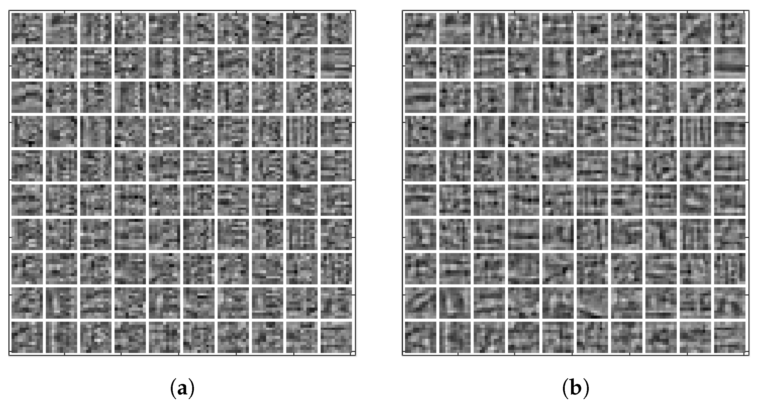
We use the following parameter values to compare the two methods in the test: $\alpha =1$, $\eta =0.1$, $\beta =1$. For the stopping criteria, we set ${ϵ}_l={ϵ}_r=0.001$ in Algorithm 1. We verified the algorithm using MATLAB 2019(a) version. When the size of the dictionary to be learned in the algorithm is small, the calculation of the proposed method can be completed faster. However, if the algorithm has a larger dictionary size, the reflectance function can be more complex, and the computational complexity will increase; therefore, we need to choose an appropriate dictionary size. In this paper, we experimentally set the size of the dictionary to $11\times 11$ and use 100 filters ($11\times 11\times 100$), as seen in Figure 3. To generate the general dictionary for large-scale image data, we use 2000 images from ImageNet [23]. As seen here, Figure 3a without SVD and Figure 3b with SVD are similar in appearance, but the dictionary with SVD includes more general features that yield better reconstruction results (Section 4.1 and Section 4.2). It also looks simpler and closer to the basis by using SVD. We collected training and test images for our experiment from [24,25], which was publicly released.

4.1. Real Image

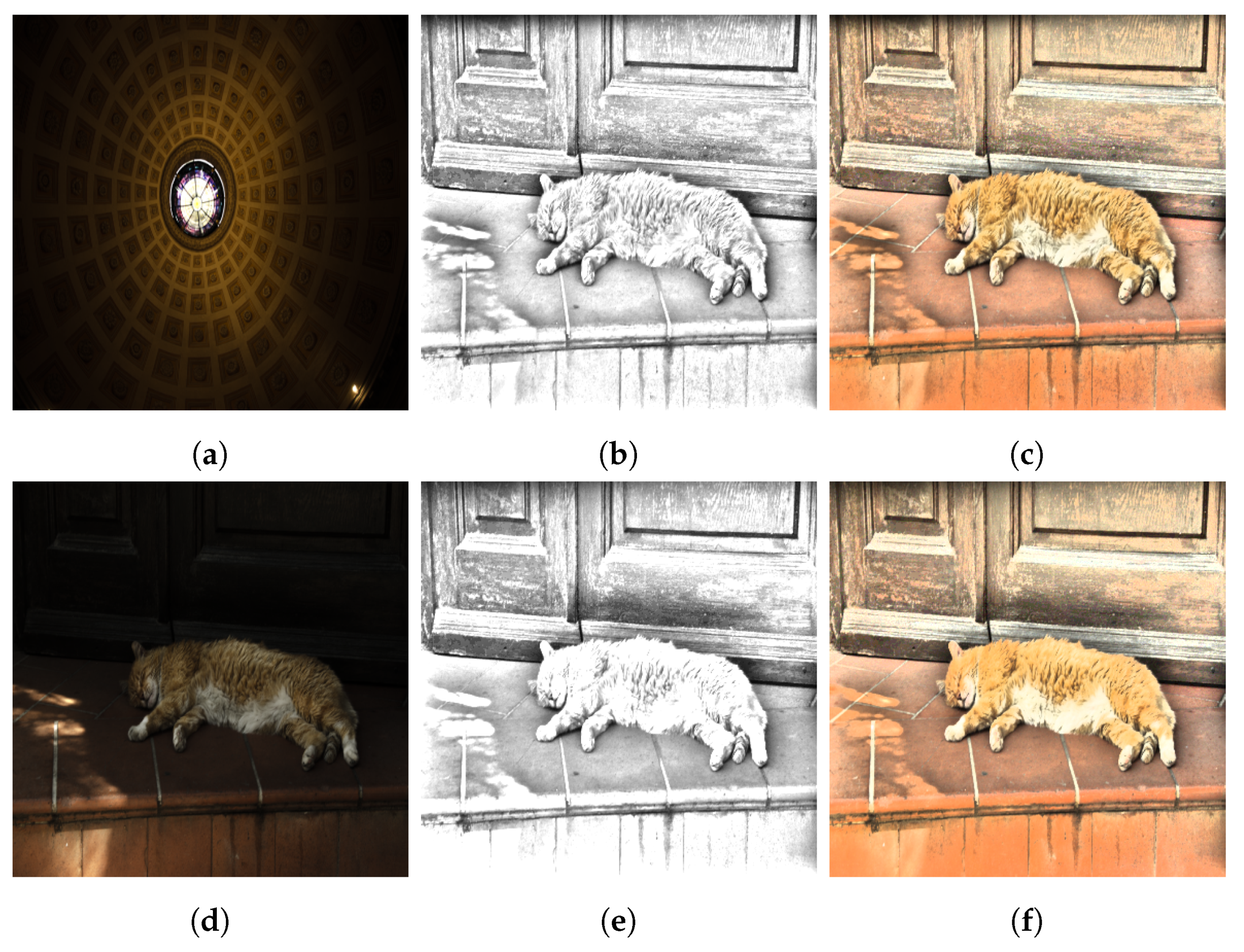
As a first experiment with a real image, we test an image with a complex structure using a dictionary learned from an image with a simple structure. By comparing this with the dictionary of sparse coding and the dictionary of CSC, we can see that the reflectance dictionary of CSC is superior to sparse coding. Through the learned dictionary using Figure 4a, the reflectance and enhancement images can be obtained through each CSC and sparse coding. Since the image used in training and the image used in the test in a single image are different, the separation of illumination and reflectance through CSC and sparse coding is not good. Although separation through CSC is not complete, it still yields better results than sparse coding. The reflectance of Figure 4b and the enhancement image of Figure 4c obtained through the CSC show that the details are better restored in the cat’s hair and texture.

Second, in Figure 5, the results of sparse coding in a single image, CSC in a single image, CSC in generating a general dictionary through large datasets, SVD-CSC in a single image and SVD-CSC in generating a general dictionary through large datasets are compared. These comparisons help contrast the performance of the general dictionary generated from large datasets to a single image dictionary. Figure 1a is an original image used as a training and test image for single image sparse coding, single image CSC, and single image SVD-CSC. In addition, it is used as a test image in the general dictionary. As shown in Figure 5c, the result of using SVD-CSC in a single image had a better quality with regard to image contrast than the result using a general dictionary. However, this difference is minimal, and Figure 5e using general dictionary in SVD-CSC also show good results. Figure 5e using the SVD-CSC general dictionary looks almost the same as Figure 5b using the CSC single dictionary. This is because SVD is not used for training in large datasets, and thus, important basis data is not extracted and used in the iteration. Therefore, only the cost function value of the reflectance function itself is minimized, and local reflectance differences are not preserved.

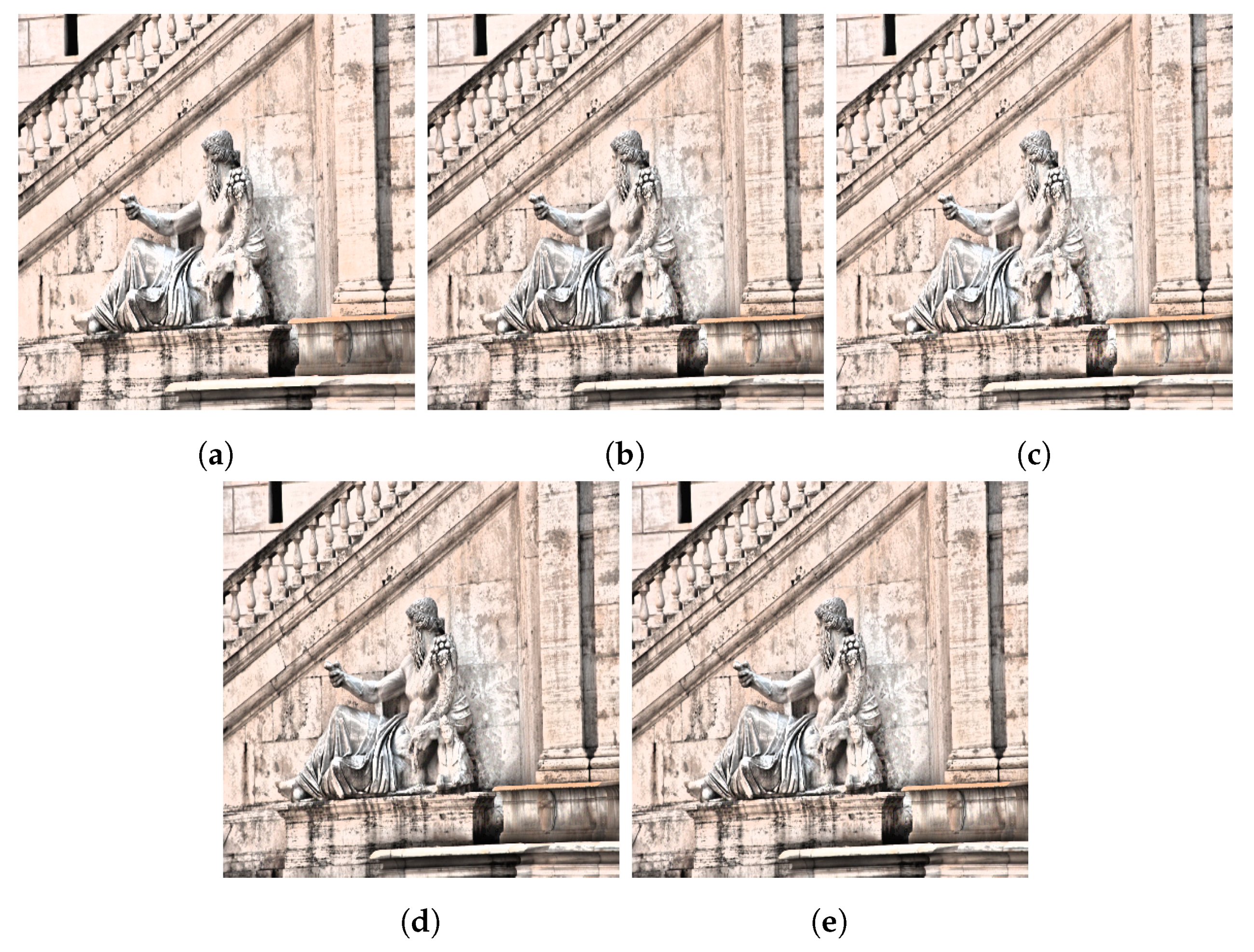
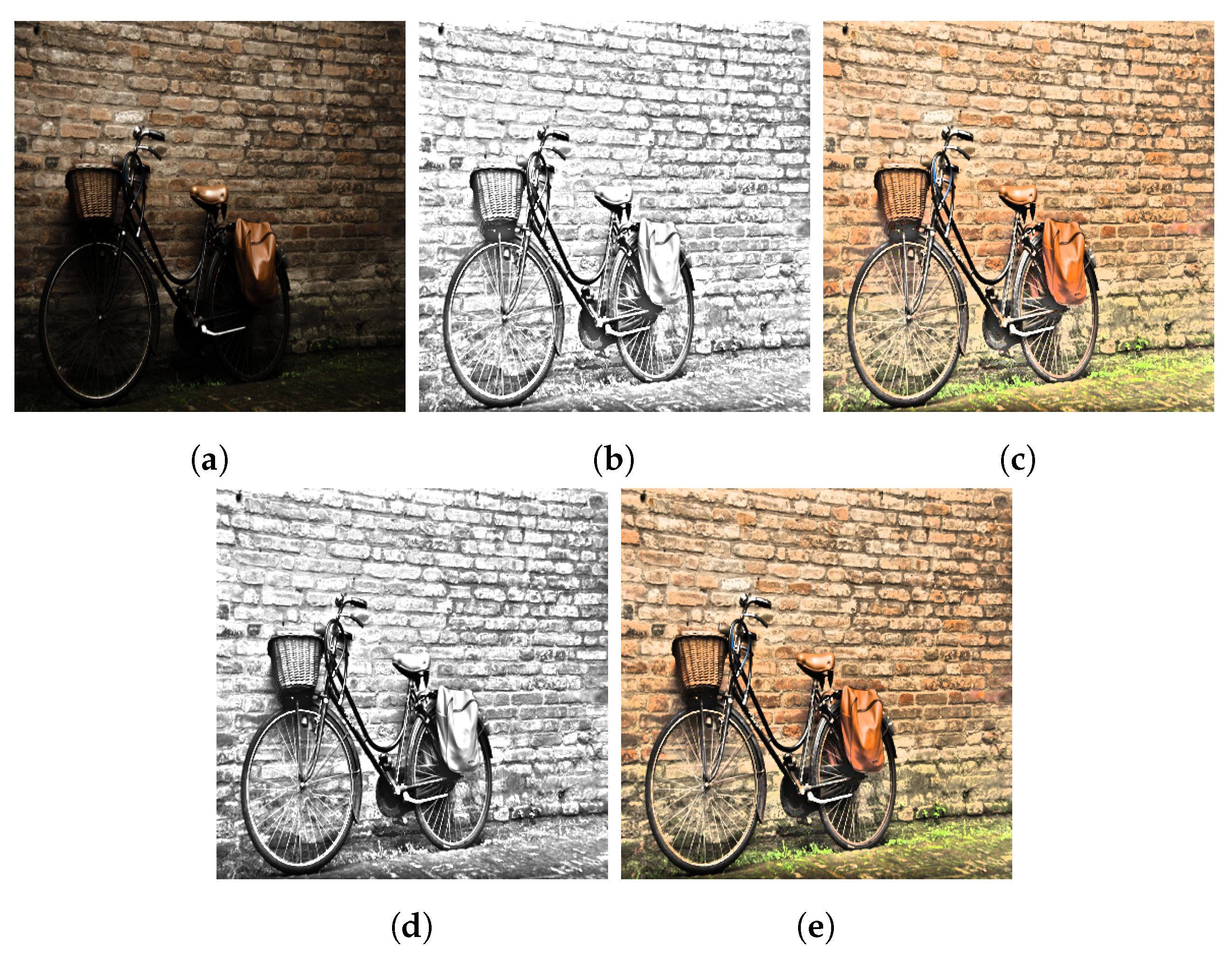
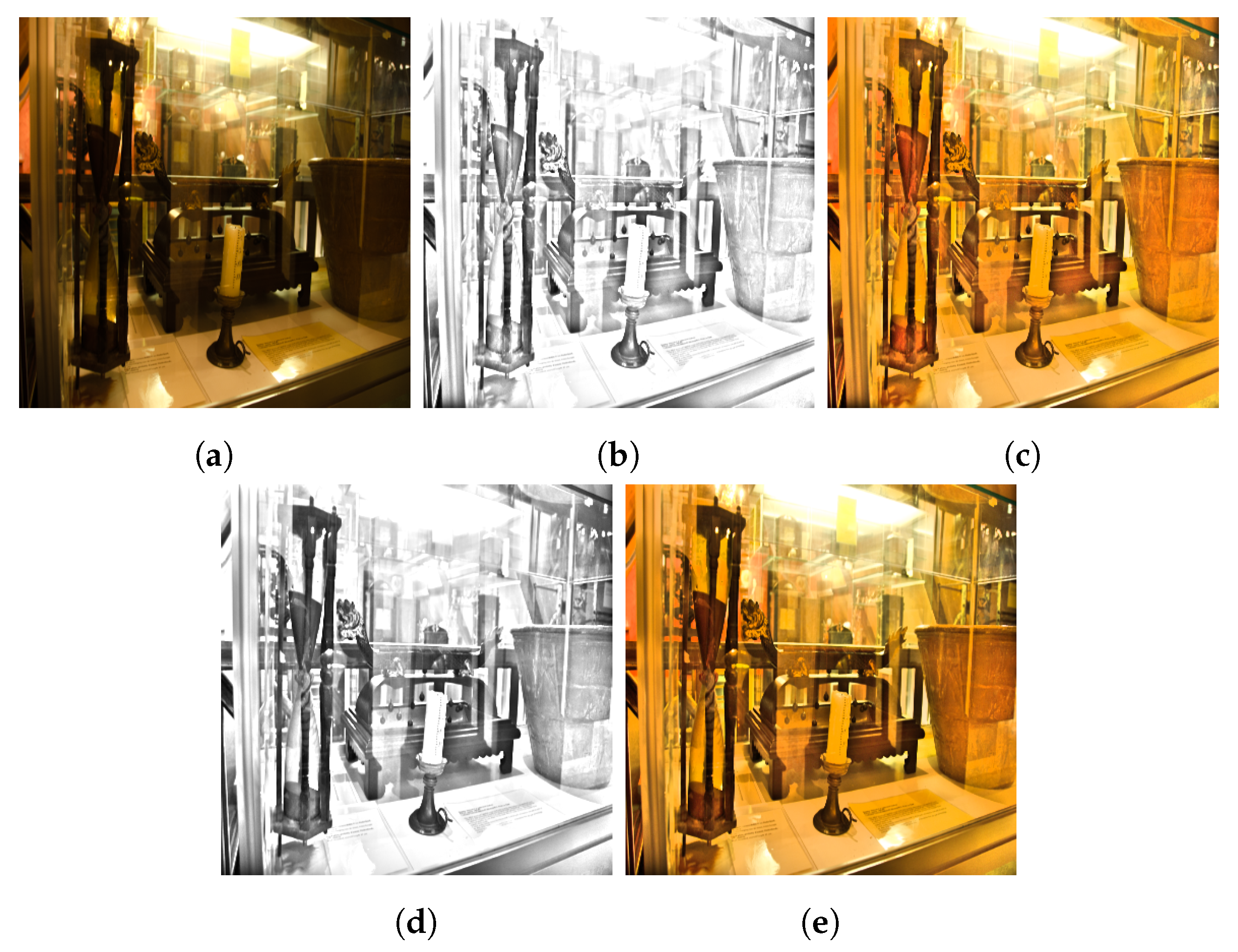
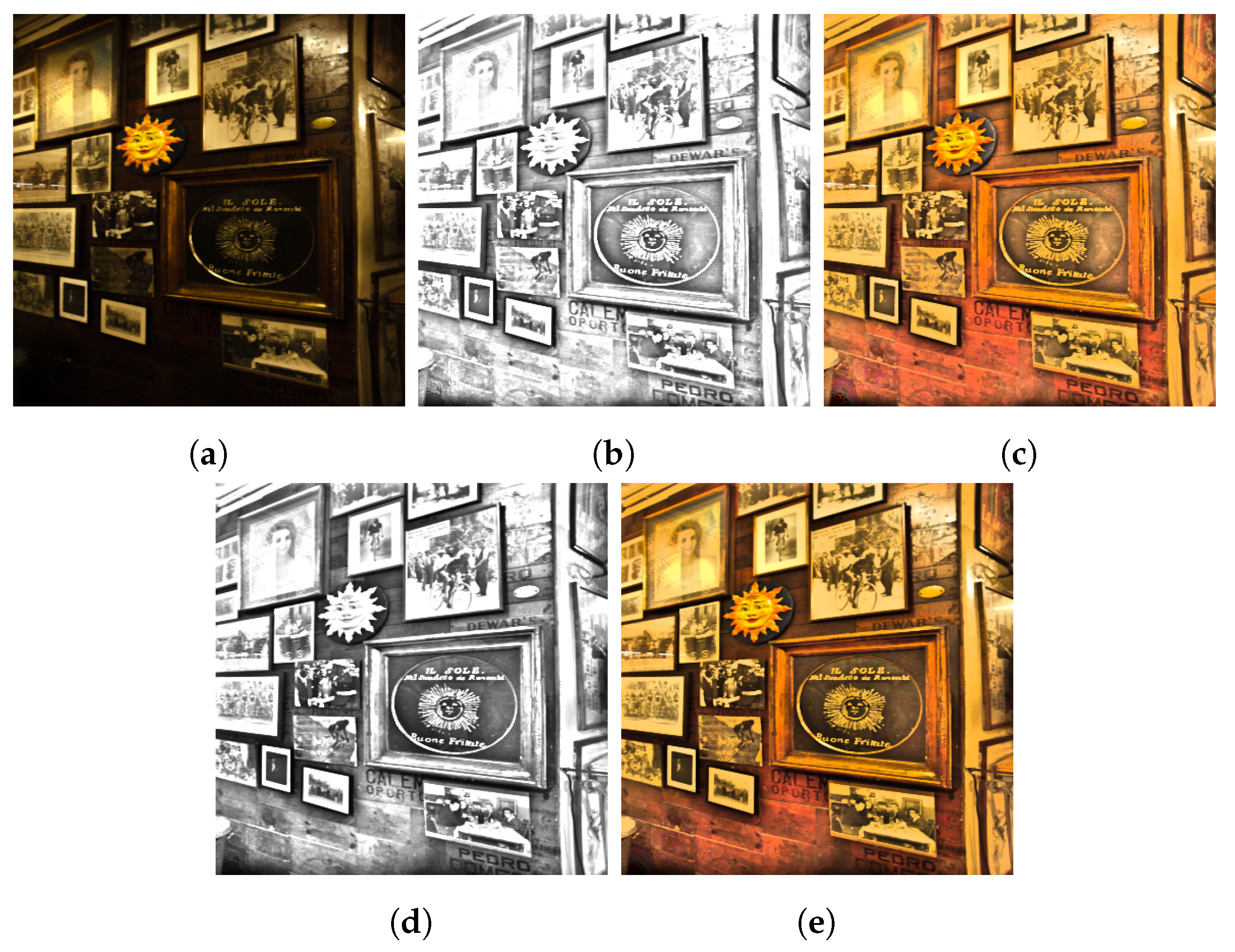
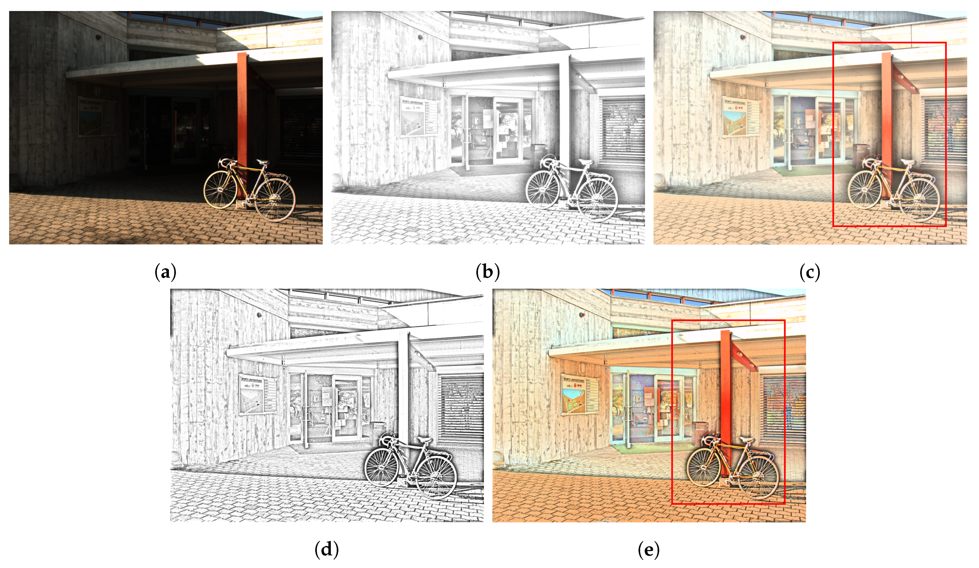
Third, we compare the SVD-CSC method with the CSC method without SVD. We show through this comparison that a dictionary using SVD can be more general than the one without SVD. As mentioned before, both dictionaries were trained with ImageNet [23] datasets. In Figure 6, Figure 7 and Figure 8, the results of the general dictionary through SVD-CSC have better image quality than those without SVD. In particular, the SVD-CSC shows better local reflectance than the CSC, when looking at the wheels of the bicycle in Figure 6, the hourglass and candlestick in Figure 7, and the frames in Figure 8. As mentioned earlier, this difference is even more pronounced in the absence of SVD, especially in terms of local reflection, because dictionaries do not contain important information, but are only directed at minimizing the energy in the least-squares problem. On the other hand, SVD-CSC generates a dictionary using SVD to decompose on the best basis in the least-squares problem.

Additionally, we examine the effect of SVD-CSC by reconstructing the reflectance from a dictionary of limited memory. For this purpose, we compare the results when the allowable memory is altered by changing the size of the filter. If the size of the filter is reduced, the elements constituting the dictionary are reduced. Consequently, each filter compresses and expresses information more clearly than when the filter size is large, and when reconstructing reflectance from such information, each filter must have more important information such as the basis of SVD than the preceding one to obtain better reconstruction results. In Figure 9a, it is seen that when using $5\times 5\times 100$ filters, the large data CSC does not express the local reflectance well.Meanwhile, the large data SVD-CSC in Figure 9b does not express perfect local reflectance, but it shows better results than the large data CSC. When using $15\times 15\times 100$ filters in Figure 9c,d, both large data CSC and large data SVD-CSC have sufficient information, and hence, they show similar results. Therefore, the proposed large data SVD-CSC method can achieve better reconstruction results by constructing a compact dictionary with limited memory.

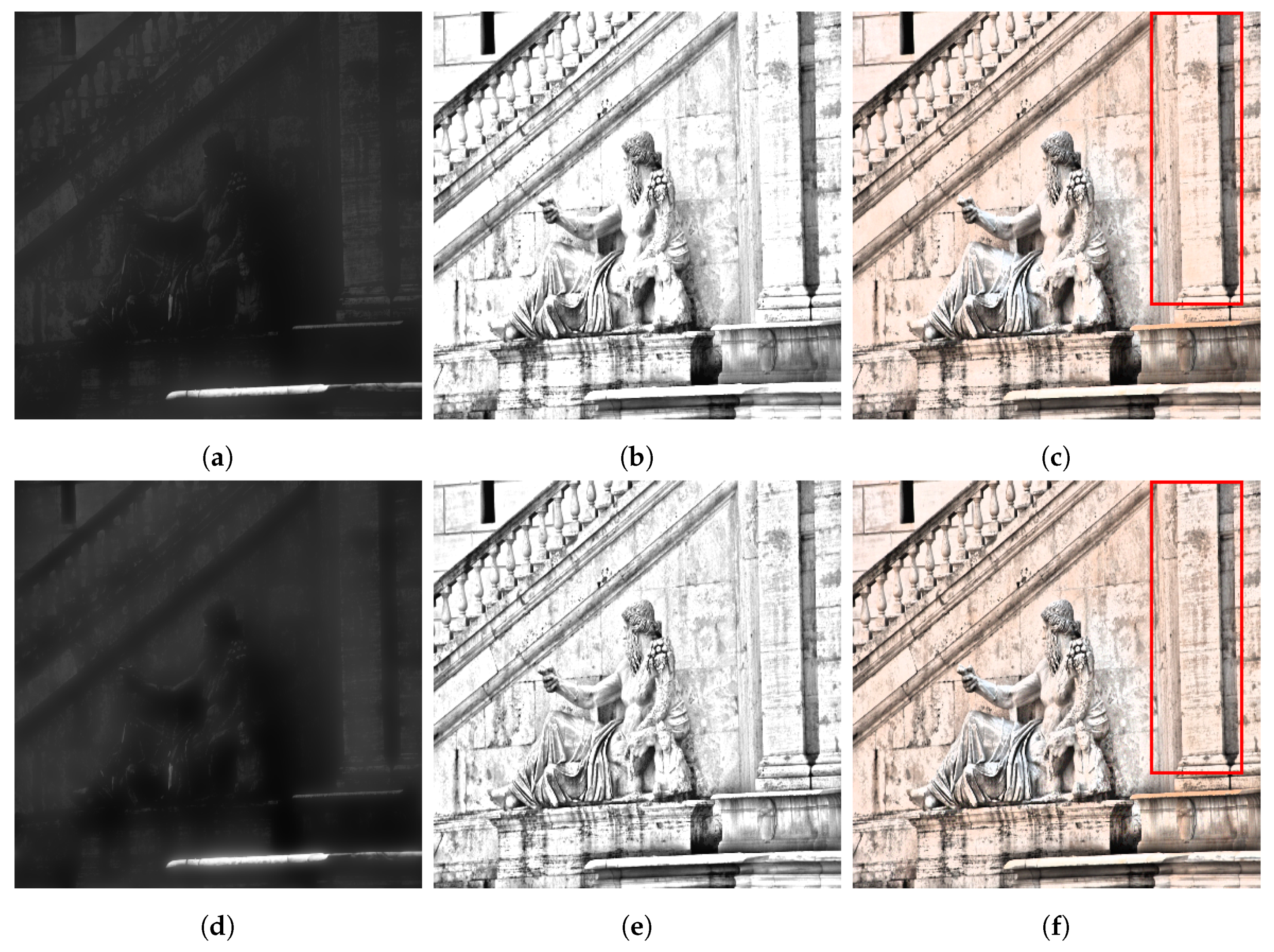
In Figure 5, Figure 6, Figure 7 and Figure 8, we show the image enhancement effect in low-light image. Finally, we show that high quality reflectance images can be obtained by removing a halo artifact from image reconstruction. A common problem with Retinex-based algorithms is the appearance of a halo artifact around the high-contrast areas owing to the rapid change in illumination. The halo artifact are shown in the red box in Figure 10. As shown in Figure 10c, the halo artifact usually appear due to the smoothness conditions of illumination of the Retinex model [16]. However, in Figure 10e our proposed method can reduce this artifact because the reflectance can be reconstructed in more detail. Therefore, our proposed method can reduce a halo artifact while using limited memory in these reconstruction applications, and acquire high quality images with enhanced edges and texture such as super resolution.

Objective Evaluation

A blind image quality assessment called natural image quality evaluator (NIQE) [26] was used to evaluate the enhanced results. A lower NIQE value represents a higher image quality. Since NIQE evaluates only the naturalness of image assessment, we used another color image assessment called auto regressive-based image sharpness metric (ARISM) [27]. In

Table 1. Objective evaluation for Retinex algorithm (11 × 11 × 100 filters).

Method		Sparse Coding [17]	Single Image CSC [18]	Single Image SVD-CSC	Large Data CSC	Large Data SVD-CSC
NIQE	Figure 5	5.5215	4.7281	4.6913	4.9423	4.7617
	Figure 6	7.2126	5.2011	4.8745	5.9401	5.4191
	Figure 7	4.8099	3.6200	3.2708	4.0044	3.6144
	Figure 8	4.9710	3.6874	3.4015	4.1226	3.6671
ARISM	Figure 5	4.2104	3.6534	3.6087	3.7988	3.7133
	Figure 6	4.6012	3.5023	3.4423	3.8546	3.5511
	Figure 7	3.1248	2.7981	2.6559	2.9061	2.7689
	Figure 8	3.4180	2.8211	2.6881	3.0580	2.8338

, the large data SVD-CSC method had a lower score on NIQE/ARISM than the sparse coding and large data CSC methods; thus, our method is shown to have a good balance and performance. In addition, the large data SVD-CSC method has a superior or similar performance to the single image CSC, and a lower performance than the single image SVD-CSC, but without a significant difference. Therefore, through objective evaluation, we showed that the general dictionary of large data SVD-CSC method has a robust performance in most cases.

We reconstruct the reflectance from the limited memory dictionary illustrated in Figure 5, Figure 6, Figure 7 and Figure 8 to confirm the effect of SVD-CSC. The smaller the filter size of the dictionary, the more the compression rate, which adversely affects the performance when it reconstructs reflectance and subsequently, leads to bad results. Nevertheless, our proposed SVD-CSC method represents an effective objective performance indicator. In

Table 2. Objective evaluation by filter size.

Filter Size		5 × 5 × 100 Filters		11 × 11 × 100 Filters		15 × 15 × 100 Filters
Method		Large Data CSC	Large Data SVD-CSC	Large Data CSC	Large Data SVD-CSC	Large Data CSC	Large Data SVD-CSC
NIQE	Figure 5	5.4092	5.0324	4.9423	4.7617	4.7252	4.7053
	Figure 6	7.2085	6.1543	5.9401	5.4191	5.2118	5.1904
	Figure 7	4.6962	4.1081	4.0044	3.6144	3.4139	3.3392
	Figure 8	4.8696	4.2718	4.1226	3.6671	3.5627	3.4919
ARISM	Figure 5	3.9813	3.8085	3.7988	3.7133	3.6821	3.6226
	Figure 6	4.5274	4.0021	3.8546	3.5511	3.5015	3.4920
	Figure 7	3.2778	2.9963	2.9061	2.7689	2.7254	2.7114
	Figure 8	3.4842	3.1081	3.0580	2.8338	2.7121	2.7099

, when the filter size is $15\times 15$, CSC and SVD-CSC express reflectance with sufficient information, and both show similar results that are good. However, when the filter size is $5\times 5$, the performance of the CSC is greatly reduced, whereas the SVD-CSC shows similar performance to the $11\times 11$ filter CSC. Therefore, it can be seen that the proposed SVD-CSC can be effectively applied when the compression ratio is high.

4.2. Synthesis Image

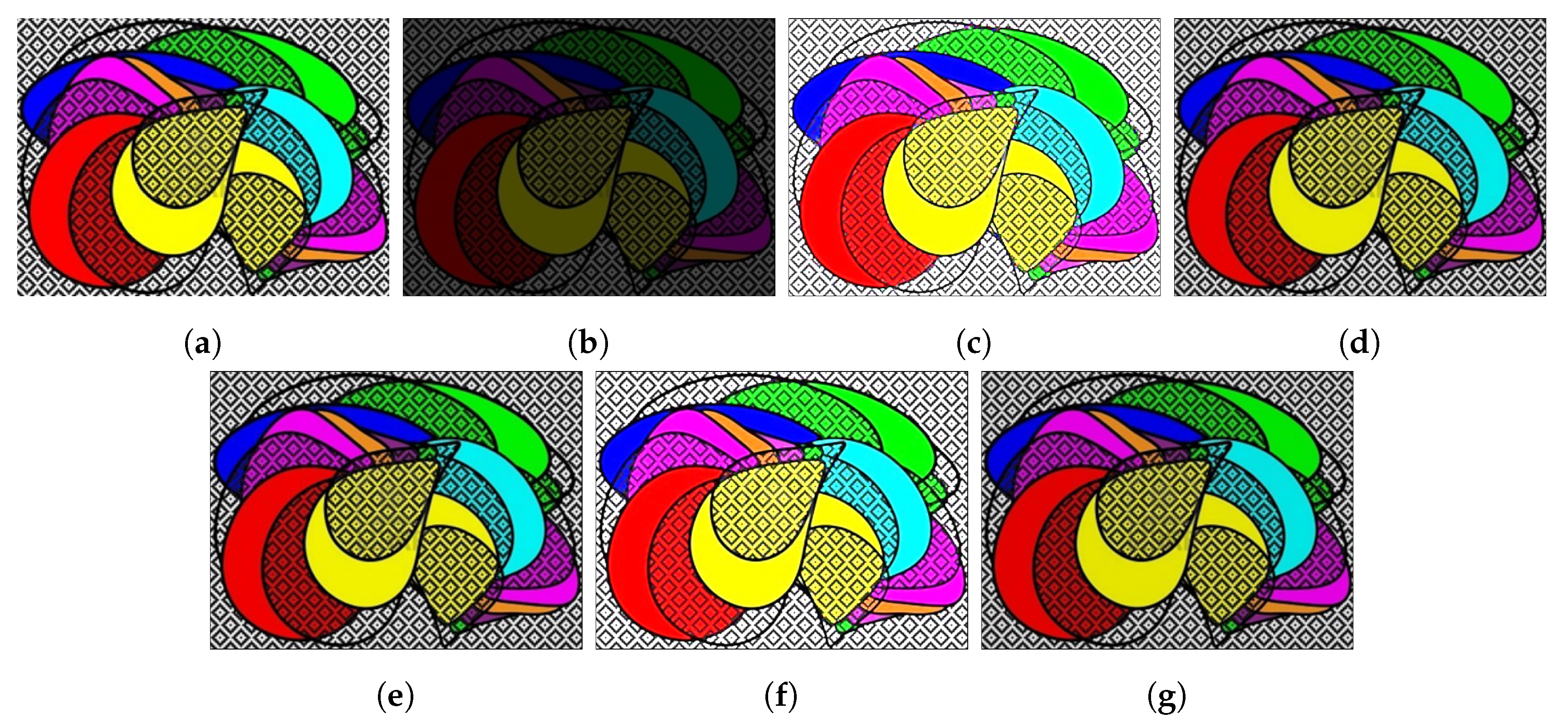
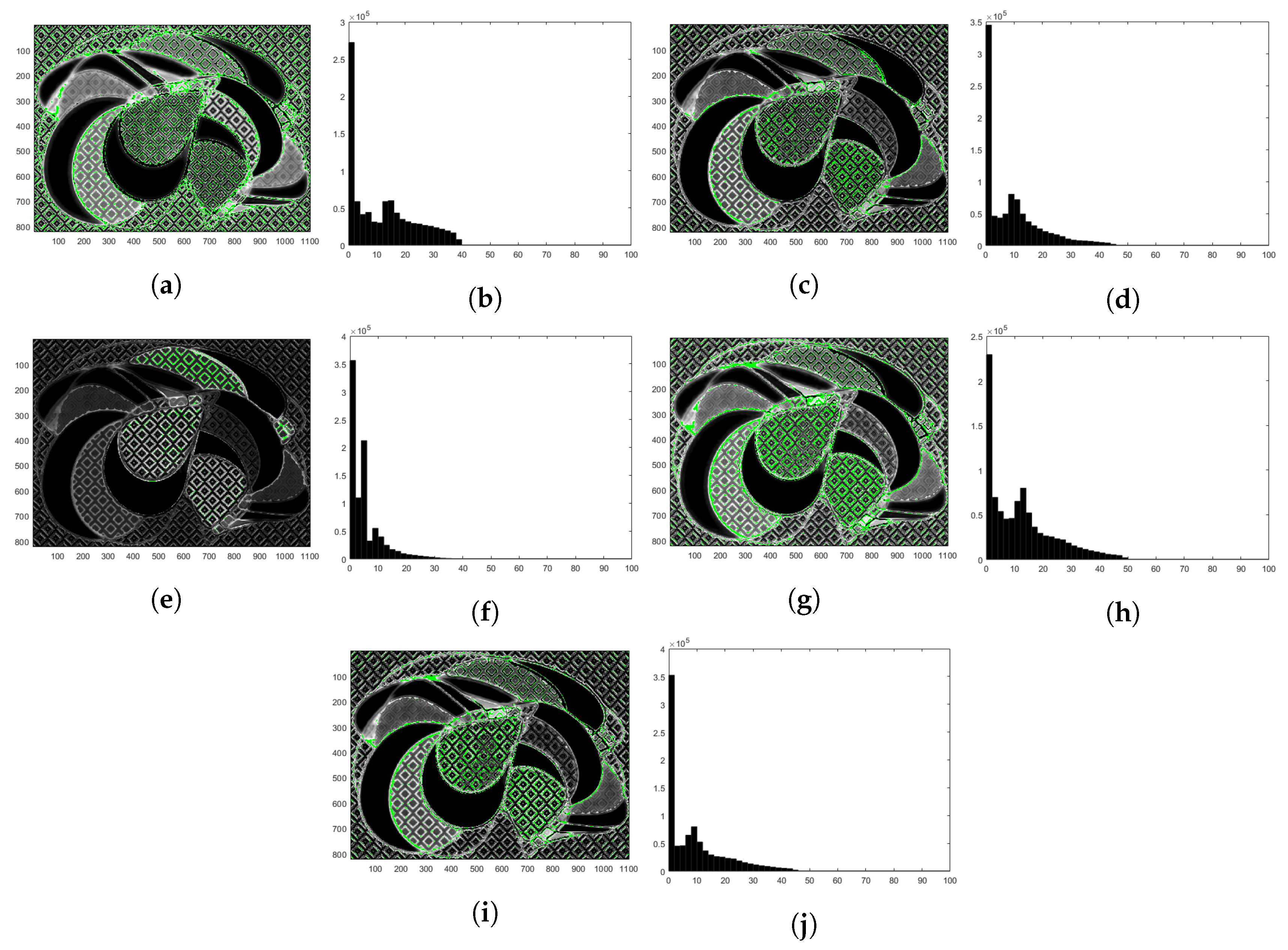
We compare the performance of the proposed SVD-CSC and other methods with a synthesized image. Figure 11 shows the results of image tests using an image with uniformly dark colors and the same degrees of illumination. From Figure 11b, image enhancement results shown in Figure 11c–g were obtained using sparse coding, single image CSC, single image SVD-CSC, large data CSC, and large data SVD-CSC methods, respectively. In Figure 12, we compare the methods using the S-CIELAB color metric [28], which includes a spatial processing step, and is useful and efficient for measuring color reproduction errors in digital images. We show the S-CIELAB errors between Figure 11a and the sparse coding results in Figure 11c, between Figure 11a and the single image CSC results in Figure 11d, between Figure 11a and the single image SVD-CSC results in Figure 11e, between Figure 11a and the large data CSC results in Figure 11f, and between Figure 11a and the large data SVD-CSC results in Figure 11g. Figure 12a,c,e,g,i show a green color when the S-CIELAB error exceeds 30 units. Figure 12b,d,f,h,j show the histogram distribution of the S-CIELAB error. The S-CIELAB error histogram distributions give the numbers of pixels per error unit. In this test, the S-CIELAB error values for the proposed method (SVD-CSC) indicate that 8.1% of the image exceeded 30 units, whereas 22.9%, 7.9%, 6.4%, and 13.8% of the image exceeded 30 units with sparse coding, single image CSC, single image SVD-CSC, and large data CSC respectively. Quantitatively, the error of single image SVD-CSC is the least, but the dictionary created in this method cannot be used in general. On the other hand, in the case of the large data SVD-CSC, the learned dictionary can be used robustly in general, with performance close to that of the single image SVD-CSC.

5. Conclusions

In this paper, we proposed Retinex based image enhancement method via CSC. To realize this, the reflectance function of the Retinex algorithm was designed through CSC. In addition, we applied a SVD to the proposed reflectance function, and a dictionary closer to the basis was constructed. Through this, the Retinex algorithm was designed to preserve more details than the existing methods, and the object function also contributed to the improved quality of the separated image. We also showed that by learning a dictionary from large datasets, we can use a general dictionary without learning a new dictionary from any input image. As shown in the experimental results, the general dictionary is robust and performs adequately for both real and synthetic images. Although we showed that the reflectance dictionary can be effectively constructed using a limited memory and has general applications, it does not contain the optimal number of dictionary filters because the number of dictionary filters has been determined experimentally. Therefore, further research is required to determine the optimal number of dictionary filters for clear and accurate results.

References

1. Rizzi, A.; McCann, J.J. On the behavior of spatial models of color. In Color Imaging XII: Processing, Hardcopy, and Applications; International Society for Optics and Photonics: Bellingham, WA, USA, 2007; Volume 6493, p. 649302. [Google Scholar]
2. Palma-Amestoy, R.; Provenzi, E.; Bertalmío, M.; Caselles, V. A perceptually inspired variational framework for color enhancement. IEEE Trans. Pattern Anal. Mach. Intell. 2008, 31, 458–474. [Google Scholar] [CrossRef]
3. Ebner, M. Color Constancy; John Wiley & Sons: Hoboken, NJ, USA, 2007; Volume 7. [Google Scholar]
4. Land, E.H. The retinex theory of color vision. Sci. Am. 1977, 237, 108–129. [Google Scholar] [CrossRef]
5. Land, E.H. Recent advances in retinex theory and some implications for cortical computations: Color vision and the natural image. Proc. Natl. Acad. Sci. USA 1983, 80, 5163. [Google Scholar] [CrossRef] [PubMed] [Green Version]
6. Land, E.H.; McCann, J.J. Lightness and retinex theory. JOSA 1971, 61, 1–11. [Google Scholar] [CrossRef] [PubMed]
7. McCann, J.J.; Parraman, C.E.; Rizzi, A. Pixel and spatial mechanisms of color constancy. In Color Imaging XV: Displaying, Processing, Hardcopy, and Applications; International Society for Optics and Photonics: Bellingham, WA, USA, 2010; Volume 7528, p. 752803. [Google Scholar]
8. Ng, M.K.; Wang, W. A total variation model for Retinex. SIAM J. Imaging Sci. 2011, 4, 345–365. [Google Scholar] [CrossRef]
9. Kimmel, R.; Elad, M.; Shaked, D.; Keshet, R.; Sobel, I. A variational framework for retinex. Int. J. Comput. Vis. 2003, 52, 7–23. [Google Scholar] [CrossRef]
10. Bertalmío, M.; Caselles, V.; Provenzi, E. Issues about retinex theory and contrast enhancement. Int. J. Comput. Vis. 2009, 83, 101–119. [Google Scholar] [CrossRef]
11. Morel, J.M.; Petro, A.B.; Sbert, C. Fast implementation of color constancy algorithms. In Color Imaging XIV: Displaying, Processing, Hardcopy, and Applications; International Society for Optics and Photonics: Bellingham, WA, USA, 2009; Volume 7241, p. 724106. [Google Scholar]
12. Rahman, Z.u.; Jobson, D.J.; Woodell, G.A. Retinex processing for automatic image enhancement. J. Electron. Imaging 2004, 13, 100–111. [Google Scholar]
13. Morel, J.M.; Petro, A.B.; Sbert, C. A PDE formalization of Retinex theory. IEEE Trans. Image Process. 2010, 19, 2825–2837. [Google Scholar] [CrossRef] [PubMed]
14. Finlayson, G.D.; Hordley, S.D.; Drew, M.S. Removing shadows from images using retinex. In Color and Imaging Conference; Society for Imaging Science and Technology: Bellingham, WA, USA, 2002; Volume 2002, pp. 73–79. [Google Scholar]
15. Ma, W.; Osher, S. A TV Bregman iterative model of Retinex theory. Inverse Probl. Imaging 2012, 6, 697. [Google Scholar] [CrossRef]
16. Yoon, J.; Choi, J.; Choe, Y. Efficient image enhancement using sparse source separation in the Retinex theory. Opt. Eng. 2017, 56, 113103. [Google Scholar] [CrossRef]
17. Chang, H.; Ng, M.K.; Wang, W.; Zeng, T. Retinex image enhancement via a learned dictionary. Opt. Eng. 2015, 54, 013107. [Google Scholar] [CrossRef]
18. Yoon, J.; Choe, Y. Retinex based reflectance decomposition using convolutional sparse coding. Trans. Korean Inst. Electr. Eng. 2020, 69, 486–494. [Google Scholar] [CrossRef]
19. Zeiler, M.D.; Krishnan, D.; Taylor, G.W.; Fergus, R. Deconvolutional networks. In Proceedings of the 2010 IEEE Computer Society Conference on Computer Vision and Pattern Recognition, San Francisco, CA, USA, 13–18 June 2010; pp. 2528–2535. [Google Scholar]
20. Heide, F.; Heidrich, W.; Wetzstein, G. Fast and flexible convolutional sparse coding. In Proceedings of the IEEE Conference on Computer Vision and Pattern Recognition, Boston, MA, USA, 7–12 June 2015; pp. 5135–5143. [Google Scholar]
21. Choudhury, B.; Swanson, R.; Heide, F.; Wetzstein, G.; Heidrich, W. Consensus convolutional sparse coding. In Proceedings of the IEEE International Conference on Computer Vision, Venice, Italy, 22–29 October 2017; pp. 4280–4288. [Google Scholar]
22. Boyd, S.; Parikh, N.; Chu, E.; Peleato, B.; Eckstein, J. Distributed optimization and statistical learning via the alternating direction method of multipliers. Found. Trends Mach. Learn. 2011, 3, 1–122. [Google Scholar] [CrossRef]
23. Deng, J.; Dong, W.; Socher, R.; Li, L.J.; Li, K.; Fei-Fei, L. Imagenet: A large-scale hierarchical image database. In Proceedings of the 2009 IEEE Conference on Computer Vision and Pattern Recognition, Miami, FL, USA, 20–25 June 2009; pp. 248–255. [Google Scholar]
24. Wei, C.; Wang, W.; Yang, W.; Liu, J. Deep retinex decomposition for low-light enhancement. arXiv 2018, arXiv:1808.04560. [Google Scholar]
25. Meylan, L.; Susstrunk, S. Bio-inspired color image enhancement. In Human Vision and Electronic Imaging IX; International Society for Optics and Photonics: Bellingham, WA, USA, 2004; Volume 5292, pp. 46–56. [Google Scholar]
26. Mittal, A.; Soundararajan, R.; Bovik, A.C. Making a “completely blind” image quality analyzer. IEEE Signal Process. Lett. 2012, 20, 209–212. [Google Scholar] [CrossRef]
27. Gu, K.; Zhai, G.; Lin, W.; Yang, X.; Zhang, W. No-reference image sharpness assessment in autoregressive parameter space. IEEE Trans. Image Process. 2015, 24, 3218–3231. [Google Scholar] [PubMed]
28. Zhang, X.; Wandell, B.A. A spatial extension of CIELAB for digital color image reproduction. In SID International Symposium Digest of Technical Papers; Society for Information Display: Campbell, CA, USA, 1996; Volume 27, pp. 731–734. [Google Scholar]
Figure 1. Single image dictionary: (a) Training image; (b) Sparse coding dictionary in single image [17]; (c) CSC dictionary in single image.
Applsci 10 04395 g001
Figure 2. The result of applying the Retinex algorithm from the single image dictionary in Figure 1: (a) SCR [17] illumination; (b) SCR reflectance; (c) Image enhancement through SCR; (d) CSC Retinex [18] illumination; (e) CSC Retinex reflectance; (f) Image enhancement through CSC Retinex.
Applsci 10 04395 g002
Figure 3. Proposed Retinex algorithm dictionary; (a) Our CSC dictionary in large datasets, (b) Our SVD-CSC dictionary in large datasets.
Applsci 10 04395 g003
Figure 4. Results of using different images for training and test in a single image: (a) Training image; (b) Reflectance using CSC dictionary; (c) Image enhancement using CSC dictionary; (d) Original Test image; (e) Reflectance using sparse coding dictionary; (f) Image enhancement using sparse coding dictionary.
Applsci 10 04395 g004
Figure 5. Comparison of single image dictionary and large datasets general dictionary in enhancement image: (a) Image enhancement using SCR same as Figure 2c; (b) Image enhancement using CSC Retinex, same as Figure 2f; (c) Image enhancement using CSC general dictionary; (d) Image enhancement using SVD-CSC single dictionary; (e) Image enhancement using SVD-CSC general dictionary.
Applsci 10 04395 g005
Figure 6. Comparison of SVD-CSC and CSC methods without SVD: (a) Original test image; (b) Reflectance using CSC general dictionary; (c) Image enhancement using CSC general dictionary; (d) Reflectance using SVD-CSC general dictionary; (e) Image enhancement using SVD-CSC general dictionary.
Applsci 10 04395 g006
Figure 7. Comparison of SVD-CSC and CSC methods without SVD: (a) Original test image; (b) Reflectance using CSC general dictionary; (c) Image enhancement using CSC general dictionary; (d) Reflectance using SVD-CSC general dictionary; (e) Image enhancement using SVD-CSC general dictionary.
Applsci 10 04395 g007
Figure 8. Comparison of SVD-CSC and CSC methods without SVD: (a) Original test image; (b) Reflectance using CSC general dictionary; (c) Image enhancement image using CSC general dictionary; (d) Reflectance using SVD-CSC general dictionary; (e) Image enhancement image using SVD-CSC general dictionary.
Applsci 10 04395 g008
Figure 9. Comparison of reconstruction results by filter size; (a) 5 × 5 × 100 filters CSC, (b) 5 × 5 × 100 filters SVD-CSC, (c) 15 × 15 × 100 filters CSC, (d) 15 × 15 × 100 filters SVD-CSC.
Applsci 10 04395 g009
Figure 10. Comparison of high contrast image reconstruction: (a) Original test image; (b) Reflectance using [16] Retinex model; (c) Image enhancement image using [16] Retinex model; (d) Reflectance using SVD-CSC general dictionary; (e) Image enhancement image using SVD-CSC general dictionary.
Applsci 10 04395 g010
Figure 11. Comparison of various methods using S-CIELAB color metric: (a) Original image; (b) Shadow version of the original image; (c) Image enhancement by sparse coding; (d) Image enhancement by single image CSC; (e) Image enhancement by single image SVD-CSC; (f) Image enhancement by large data CSC; (g) Image enhancement by large data SVD-CSC.
Applsci 10 04395 g011
Figure 12. S-CIELAB Spatial distribution of errors and error histogram: (a) Spatial distribution of errors between Figure 11a and the sparse coding results in Figure 11c that are 30 units or higher, marked in green; (b) S-CIELAB histogram distribution between Figure 11a and the sparse coding results in Figure 11c; (c) Spatial distribution of errors between Figure 11a and the single image CSC results in Figure 11d that are 30 units or higher, marked in green; (d) S-CIELAB histogram distribution between Figure 11a and the single image CSC results in Figure 11d; (e) Spatial distribution of errors between Figure 11a and the single image SVD-CSC results in Figure 11e that are 30 units or higher, marked in green; (f) S-CIELAB histogram distribution between Figure 11a and the single image SVD-CSC results in Figure 11e; (g) Spatial distribution of errors between Figure 11a and the large data CSC results in Figure 11f that are 30 units or higher, marked in green; (h) S-CIELAB histogram distribution between Figure 11a and the large data CSC results in Figure 11f; (i) Spatial distribution of errors between Figure 11a and the large data SVD-CSC results in Figure 11g that are 30 units or higher, marked in green; (j) S-CIELAB histogram distribution between Figure 11a and the large data SVD-CSC results in Figure 11g.
Applsci 10 04395 g012