A Polarity Capturing Sphere for Word to Vector Representation

Abstract

Embedding words from a dictionary as vectors in a space has become an active research field, due to its many uses in several natural language processing applications. Distances between the vectors should reflect the relatedness between the corresponding words. The problem with existing word embedding methods is that they often fail to distinguish between synonymous, antonymous, and unrelated word pairs. Meanwhile, polarity detection is crucial for applications such as sentiment analysis. In this work we propose an embedding approach that is designed to capture the polarity issue. The approach is based on embedding the word vectors into a sphere, whereby the dot product between any vectors represents the similarity. Vectors corresponding to synonymous words would be close to each other on the sphere, while a word and its antonym would lie at opposite poles of the sphere. The approach used to design the vectors is a simple relaxation algorithm. The proposed word embedding is successful in distinguishing between synonyms, antonyms, and unrelated word pairs. It achieves results that are better than those of some of the state-of-the-art techniques and competes well with the others.

1. Introduction

Word vector embeddings seek to model each word as a multi-dimensional vector. There are many distinct benefits to modeling words as vectors. Implementing natural language processing (NLP) algorithms using machine learning models necessitates converting a textual word or sentence to a numeric format. Moreover, this conversion has to be meaningful. For example, words with similar meanings should possess vectors that are in close proximity in the embedded space. This is because such words should produce similar outputs, if applied to a machine learning model. Additionally, a word embedding of a complete dictionary will provide a complete representation of the corpus. In this, each word is assigned to its unique position in the vector space, which reflects its aggregate relations with all other words in one cohesive construct. Word vector spaces have been very useful in many applications; for example, machine translation [1], sentiment analysis [2,3,4,5], question answering [6,7], information retrieval [8,9], spelling correction [10], crowdsourcing [11], named entity recognition (NER) [12], text summarization [13,14,15], and others.

The problem of existing word vector embedding methods is that the polarity of words is not adequately considered. Two antonyms are considered polar opposites, and have to be modeled as such. However, most current methods do not deal with this issue. For example, they do not differentiate in the similarity score between two unrelated words and two opposite words.

In this work we propose a new embedding that takes into account the polarity issue. The new approach is based on embedding the words into a sphere, whereby the dot product of the corresponding vectors represents the similarity in meaning between any two words. The polar nature of the sphere is the main motivation behind such embedding since this way antonymous relations can be captured such that a word and its antonym are placed at opposite poles of the sphere. This polarity capturing feature is essential for some applications such as sentiment analysis. Recently, word embedding methods have started to pervade the sentiment analysis field, at the expense of traditional machine learning algorithms, which rely on sentiment-polarity data that are annotated manually, and expensive feature engineering. Using word embeddings, a sentence can be mapped to a number of features based on the embeddings of its words. However, these embeddings should reflect the polarity of words in order to be able to perform the sentiment analysis task. As mentioned before, this polarity issue is completely addressed in our word embedding approach.

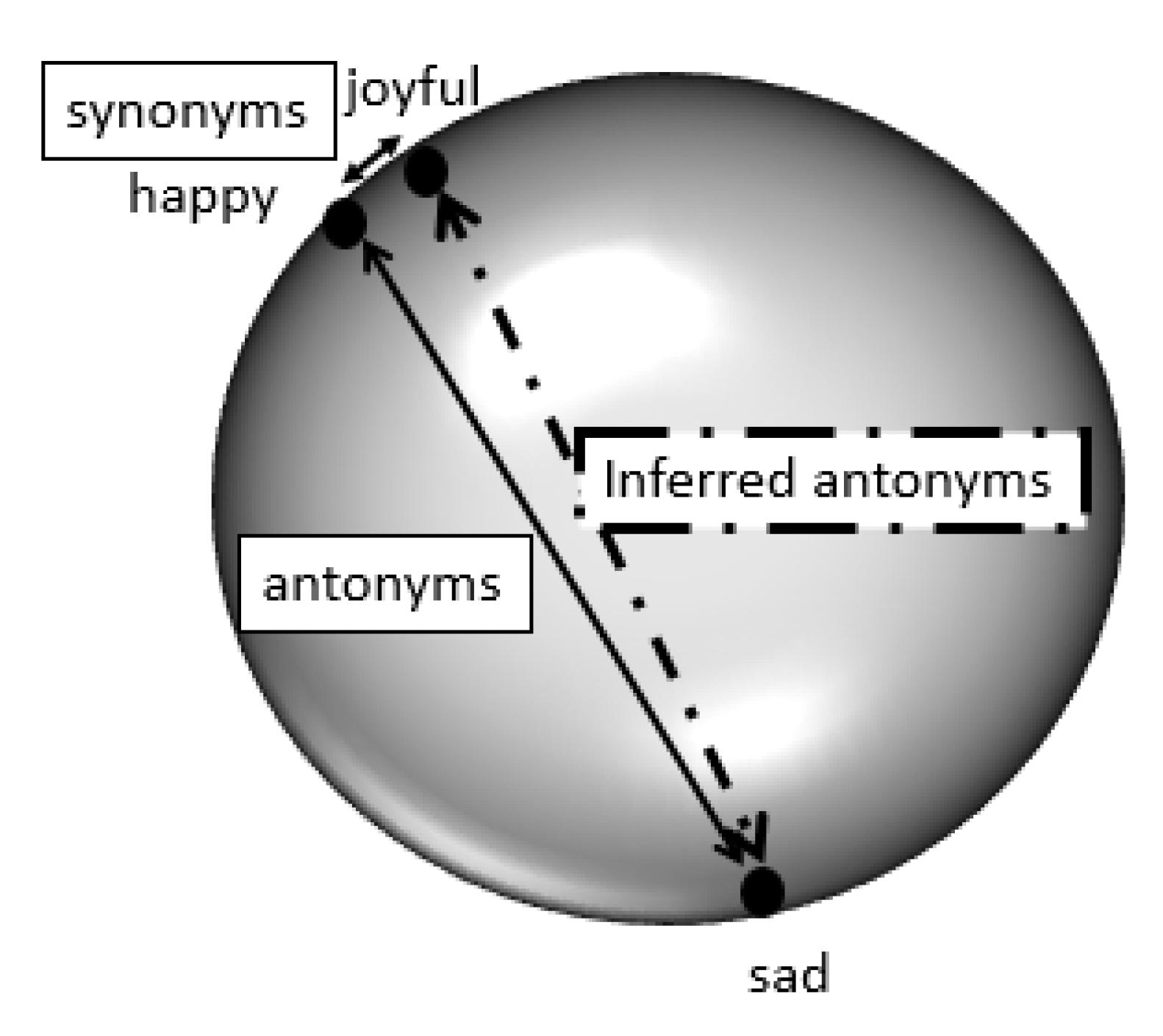
Figure 1 illustrates the concept of the proposed approach. As shown in the figure, the two vectors corresponding to the words “happy” and “joyful” have close similarity because they are synonyms. On the other hand, the vectors corresponding to “happy” and “sad” are on opposite poles and have a similarity score of −1, because they are antonyms. The algorithm can infer a new relation that “joyful” and “sad” are antonyms too, as their corresponding vectors are also placed close to opposite poles of the sphere.

Two words that are similar in meaning are assigned vectors whose similarity measure is 1. Two unrelated words will be assigned a similarity close to zero, and two antonyms are assigned similarity close to −1. In other words, we specifically consider the polarity issue and make a distinction between “opposite” and “unrelated”.

The fact that the similarity between opposing words or antonyms is close to −1 is consistent with the logically appealing fact that negation amounts to multiplying by −1. Double negation amounts to multiplying −1 twice, giving a similarity close to one (the antonym of an antonym is a synonym). In our geometry, negation can also be considered as reflection around the origin. Thus, the designed model makes logical sense. Another question to investigate is whether the unrelated words should have similarity close to zero. The answer is yes. It is logical that unrelated words, e.g., “train” and “star”, would have their vectors far away from each other, because of our principle that vector similarities or closeness should reflect relatedness. This is consistent with the theory that at a high dimension, the dot product of randomly occurring unit vectors on the sphere is close to zero [16]. The algorithm has a number of beneficial features:

• The proposed algorithm is a very simple relaxation algorithm, and it converges very well and fast. It is simpler than the typically used word to vector design methods, such as neural networks or deep networks.
• We believe that embedding the vectors into a sphere provides a natural representation, unlike distributional models for learning word vector representations and other co-occurrence-based models. Some of these models often fail to distinguish between synonyms and antonyms, since antonymous words occur in similar context the same way synonymous words do. Other models fail to distinguish between antonymous word pairs and unrelated word pairs.
• The learned word vectors can always be continuously augmented. The database can flexibly be extended to include more words by simply feeding the algorithm with more word pairs with the desired target similarity scores. The algorithm guarantees that these new vectors will be placed correctly with regard to the existing vectors.
• Composite words can also be handled by our algorithm. This is because any word pair with the desired similarity score can be fed into the algorithm . For example, “old-fashioned” is an expression that combines two words: “old” and “fashion”; this combined expression can be given to our algorithm as a synonym to a word that conveys its meaning; e.g., “outdated”.
• Generally it is a supervised procedure. The designer typically gives synonyms/antonyms from thesauri or other sources. However, it could also be designed in a semi-supervised setting. This means that in addition to the user-defined similarity scores between the collected words, there could be many more unlabeled pairs that have to be learned from the text pieces available (for example, through co-occurrence arguments). The labeled pairs will provide some anchor around which the unlabeled pairs will organize, and are therefore essential for guiding the correct vector placements. In other words, new relations between word pairs will be inferred from existing ones.

2. Literature Review

One of the earliest word vector embeddings is the work by Mikolov et al. [17], who published the Google word2vec representations of words. Their method relies on the continuous skip-gram model for learning the vectors introduced in [18]. Finding vector representations that predict the surrounding words is the training goal of the skip-gram model. For computational efficiency, the authors have replaced the full softmax with three alternative choices, and evaluated the results for each: hierarchical softmax, noise contrastive estimation, and negative sampling. Moreover, subsampling of frequent words was introduced to speed up the training and leverage the accuracy of word representations.

Pennington et al. [19] have published another approach (called GloVe) of word vector modeling using a method that combines the benefits of the techniques of global matrix factorization and local context window. The authors have suggested the idea of learning the word vector with the ratios of co-occurrence probabilities rather than the probabilities themselves. The result is a new global log-bilinear regression model, where the model directly captures global corpus statistics.

Mikolov et al. [20] developed a model known as fastText that is based on continuous bag-of-words (cbow) used in word2vec [18]. The authors used a combination of known improvements to learn high-quality word vector representations. To obtain higher accuracy, the authors added position-dependent weights and subword features to the cbow model architecture.

Dev et al. [21] developed a technique that aligns word vector representations from different sources such as word2vec [17] and GloVe [19]. The authors extend absolute orientation approaches to work for arbitrary dimensions.

It can be noted that word2vec [17,18], GloVe [19], and fastText [20] are distributional models for learning word vector representations. Words are assigned similarity relations based on co-occurrence in text. The limitation of these models is a weakness in distinguishing antonyms from synonyms because antonymous words such as “good” and “bad” very often occur in similar contexts so their learned vectors will be close. This way it may be hard to figure out whether a pair of words is a pair of synonyms or antonyms. However, such information is crucial for some applications such as sentiment analysis. On the other hand, our approach is a simple relaxation algorithm that takes into account learning word vectors that are able to distinguish between word relations such as synonyms, antonyms, and unrelated words. It is based on embedding the vectors on the sphere. The sphere provides a natural setting for this task, because antonyms can be placed on opposite sides of the sphere. In contrast, most methods embed the vectors in the space $R^n$, which does not provide a natural way of modeling opposites. The aforementioned models rely on corpus data of huge sizes to guarantee the effectiveness of the generated vectors. In our approach, we make use of the available experts’ lexicons, dictionaries, and thesauruses, and so the similarity relations are fairly accurate, because of the expert knowledge used to construct these lexicons.

Other works include Vilnis et al. [22], who introduced density-based distributed embeddings by learning representations in the space of Gaussian distributions. Bian et al. [23] focused on incorporating morphological, syntactic, and semantic knowledge with deep learning to obtain more efficient word embeddings. Zhou et al. [24] used the category information associated with the community question answering pages as metadata. These metadata are fed to the skip-gram model to learn continuous word embeddings, followed by applying Fisher kernel to obtain fixed length vectors.

Some works introduce retrofitting to overcome the deficiencies in distributional models in representing the semantic and relational knowledge between words. Faruqui et al. [25] applied retrofitting to pre-trained word vectors from distributional models. The vectors are refined to account for the information in semantic lexicons. The method used is graph-based learning where the graph is constructed for the relations extracted from the lexicons. Jo [26] proposed extrofitting by extracting the semantic relations between words from their vectors using latent semantic analysis. The author further combined extrofitting with external lexicons for synonyms to obtain improved results.

There have been some attempts at tackling the polarity issue. Mohammad et al. [27] proposed an empirical none-word embedding approach for the detection of antonymous word pairs. The authors’ approach relies on the co-occurrence and distributional hypotheses of antonyms, stating that antonymous word pairs occur in similar contexts more often than chance. Nevertheless, these hypotheses are only useful indications but not sufficient conditions to detect antonymous words.

Lobanova [28] proposed pattern-based methods to automatically identify antonyms. The author pointed out how antonyms are useful in many NLP applications, including contradiction identification, paraphrase generation, and document summarization.

Yih et al. [29] derived the word vector representations using latent semantic analysis (LSA), with assigning signs to account for antonymy detection, and devising the polarity inducing LSA (PILSA). Yet the authors pivoted on the fact that words with least cosine similarity are indeed opposites without regard to distinguishing between unrelated word pairs, which also have low cosine similarity, and antonymous word pairs. To embed out-of-vocabulary words, the authors adopted a two stage strategy: first conducting a lexical analysis, and, if no match was found, using semantic relatedness. This strategy weakens the smoothness of extending their approach.

Again, Mohammad et al. [30] devised an empirical method that marks word pairs that occur in the same thesaurus category as synonyms and others that occur in contrasting categories as opposites. They then apply postprocessing rules, since based on their method one word pair may be marked as both synonym and antonym at the same time. The approach devised is a none-word embedding one.

Chang et al. [31] introduced multi-relational latent semantic analysis (MRLSA) that extends PILSA [29], modeling multiple word relations. The authors proposed a 3-way tensor, wherein each slice captures one particular relation. However, the model performance depends on the quality of a pivot slice (e.g., the synonym slice), which MRLSA has to choose. Motivated by this approach, Zhang et al. [32] introduced a Bayesian probabilistic tensor factorization model. Their model combined both thesauri information and existing word embeddings, though their model used pre-trained word embeddings.

Santus et al. [33] devised a new average-precision-based measure to discriminate between synonyms and antonyms. The measure is built on the paradox of “simultaneous similarity and difference between the antonyms”. The authors deduced that both synonyms and antonyms are similar in all dimensions of meaning except one. This different dimension can be identified and used for the discrimination task.

Ono et al. [34] trained word embeddings to detect antonyms. They introduced two models: a word embeddings on thesauri information (WE-T) model and a word embeddings on thesauri and distributional information (WE-TD) model. For WE-T, the authors applied an AdaGrad online learning method that uses a gradient-based update with automatically-determined learning rate. For WE-TD, the authors introduce skip-gram with negative sampling (SGNS). However, their model is trained such that synonymous and antonymous pairs have high and low similarity scores respectively. This imposes a challenge in differentiating between antonymous word pairs and unrelated word pairs since both will have low similarity scores.

Nguyen et al. [35] proposed augmenting lexical contrast information to distributional word embeddings in order to enhance distinguishing between synonyms and antonyms. Moreover, the authors extended the skip-gram model to incorporate the lexical contrast information into the objective function.

Motivated by the fact that antonyms mostly lie at close distances in the vector space, Li et al. [36] proposed a neural network model that is adapted to learn word embeddings for antonyms. These embeddings are used to carry out contradiction detection.

In most of these aforementioned antonymy construction methods the problem is that they focus mostly on this task only. For example [29,32,34] only evaluated their vectors on antonymy detection without showing the performance of these vectors on synonyms or unrelated words. The goal in these works has mainly not been to obtain a global word embedding that works for synonyms, antonyms, and unrelated words.

Word embeddings obtain the whole picture, as to the semantic relations of the words in a corpus. As such, they have many applications. For example, Zou et al. [1] proposed a method to learn bilingual embeddings to perform a Chinese–English machine translation task. Moreover, word embeddings methods are applied to sentiment analysis; Maas et al. [2] proposed a model that combines supervised and unsupervised techniques to learn word vectors that capture sentiment content. The goal was to be able to use these vectors in sentiment analysis tasks. The authors used an unsupervised probabilistic model of documents followed by a supervised model that maps a word vector to a predicted sentiment label using a logistic regression predictor that relies on sentiment annotated texts. Tang et al. [3] developed a word embedding method by training three neural networks. The method relies on encoding sentiment information in the continuous representations of words. They evaluated their method on a benchmark Twitter sentiment classification dataset. Dragoni et al. [4] employed word embeddings and deep learning to bridge the gap between different domains, thereby building a multi-domain sentiment model. Deho et al. [5] used word2vec to generate word vectors that learn contextual information. To perform sentiment analysis, the generated vectors were used to train machine learning algorithms in the form of classifiers. Question answering is another application of word embeddings; for example, Liang et al. [6] tackled the rice FAQ (frequently asked question) question-answering system. The authors proposed methods based on word2vec and LSTM (long-short term memory). The core of the system is question similarity computing, which is used to match users’ questions and the questions in FAQ. Liu et al. [7] designed a deep learning model based on word2vec to find the best answers to the farmers’ questions. Search service also exploits word embeddings; Liu et al. [9] established a model based on word embeddings to improve the accuracy of data retrieval in the cloud. Spelling correction can also be done using word embeddings. Kim et al. [10] proposed a method of correcting misspelled words in Twitter messages by using an improved Word2Vec. The authors in [11] proposed crowdsourcing where the relevance between task and worker is obtained. The proposed model involves the computation of the similarity of word vectors and the establishment of the semantic tags similar matrix database based on the Word2vec deep learning. Habibi et al. [12] proposed a method based on deep learning and statistical word embeddings to recognize biomedical named entities (NER), such as genes, chemicals, and diseases. Word embeddings have also tackled the field of text summarization; to achieve automatic summarization Kågebäck et al. [13] proposed the use of continuous vector representations as a basis for measuring similarity. Rossiello et al. [14] proposed a centroid-based method for text summarization that exploits the compositional capabilities of word embeddings.

Word embeddings have been developed for other languages as well. Zahran et al. [37] compared diverse techniques for building Arabic word embeddings, and evaluated these techniques using intrinsic and extrinsic evaluations. Soliman et al. [38] proposed the AraVec model, a pre-trained distributed word embedding project, which makes use of six different models. The authors described the used resources for building such models and the preprocessing steps involved.

3. The Proposed Method

Let $x_i={(x_{i1},\dots ,x_{iN})}^T$ be an N-dimensional vector of unity length that represents word i; i.e., $\parallel x_i\parallel =1$. The fact that the length of the vector is 1 means that the word is embedded on a sphere. The dot product between two vectors $x_i^T{x}_j$ represents the similarity between their corresponding words. For example $x_i^T{x}_j$ for the words easy and simple would be very high (close to 1). For the words easy and manageable it would also be high, but a shade lower. For the opposites easy and difficult it would be close to −1, and for unrelated words, such as easy and cat, it would be close to zero. It is well known that when picking up any two random vectors on a sphere of high dimension, their dot product will be close to zero. This means that the bulk of the words will have similarity close to zero with the word easy. Note also that because of the unit length property, the dot product $x_i^T{x}_j$ and the distance are related in a one to one way (because $\parallel x_i-x_j{\parallel }^2=\parallel x_i{\parallel }^2+{\parallel x_j\parallel }^2-2x_i^T{x}_j=2\left[1-x_i^T{x}_j\right]$).

We collect a number of words for which we estimate a similarity number, on a scale from −1 to 1. For example, for a pair of words with corresponding vectors $x_i$ and $x_j$, let the estimated similarity be $s_{ij}$. We collect a very large training set, obtained from some well-known synonym and antonym lists. For any word relations that are not covered by these lists, we add a moderately sized but typically not-large training set, mainly labeled by an expert human. The expert-labeled dataset serves as the nucleus that will guide the training using the other larger collected datasets.

We develop an algorithm that estimates the vectors $x_i$ that would yield the similarity numbers as close as possible to the given similarity numbers. We define the following error function:

$$\begin{array}{c}\hfill E=\sum _i\sum _j{w}_{ij}{\left[x_i^T{x}_j-s_{ij}\right]}^2\\ \mathrm{subject}\mathrm{to}\parallel x_i\parallel =1,i=1,\dots ,K\hfill \end{array}$$

(1)

where $w_{ij}$ is a weighting coefficient representing the confidence in the similarity estimate $s_{ij}$. For example, the word pairs labeled by an expert may have higher weighting coefficient than other word pairs in the remaining larger training set. It is hard to solve this large optimization problem if one seeks to obtain all K vectors $x_i$ at once. However, we propose a relaxation algorithm, that tackles one $x_i$ at a time. In this algorithm we focus on some $x_k$ and fix all other $x_l$’s for the time being. Then we optimize E with respect to $x_k$. This is feasible and gives a close form solution. Then, we move on to the next vector, and fix the others, optimize with respect to that vector. We continue in this manner until we complete all vectors. Then we start another cycle, and re-optimize each $x_k$, one at a time. We perform a few similar cycles until the algorithm converges.

Consider that we are focusing now on vector $x_k$, while keeping all other vectors constant. Then we can decompose the objective function in (1) into a component containing $x_k$ and other components that do not have $x_k$ in them, as follows.

$$\begin{array}{ccc}\hfill E& =& \sum _{i\ne k}\sum _{j\ne k}{w}_{ij}{\left[x_i^T{x}_j-s_{kj}\right]}^2+2\sum _{j\ne k}{w}_{kj}{\left[x_k^T{x}_j-s_{kj}\right]}^2\hfill \\ & =& R_k+2\sum _{j\ne k}{w}_{kj}{\left[x_k^T{x}_j-s_{kj}\right]}^2\hfill \end{array}$$

(2)

where $R_k$ is the term not containing $x_k$. We skipped the term $x_k^T{x}_k-s_{kk}$ because it equals zero always (the similarity between a vector and itself is 1, and the norm of any vector is enforced as 1 too). The factor 2 in the RHS is to account for the existence of $x_k$ in first summation, and in the second summation. The optimization will now focus on optimizing the second term in the summation. Using a Lagrange multiplier to take into account the unity norm constraint, we formulate the augmented objective function:

$$V=R_k+2\sum _{j\ne k}{w}_{kj}{\left[x_k^T{x}_j-s_{kj}\right]}^2-\lambda \left(x_k^T{x}_k-1\right)$$

(3)

where $\lambda$ is the Lagrange multiplier. For simplicity, let us redefine quantities in a way to skip the factor of 2 in the equation. Simplifying, we get:

$$\begin{array}{ccc}\hfill V& =& R_k+\sum _{j\ne k}{w}_{kj}\left[x_k^T{x}_j{x}_j^T{x}_k-2x_j^T{s}_{kj}{x}_k+s_{kj}^2\right]\hfill \\ & & -\lambda x_k^T{x}_k+\lambda \hfill \\ & =& R_k+x_k^T\left(\sum _{j\ne k}{w}_{kj}{x}_j{x}_j^T\right)x_k-\left(2\sum _{j\ne k}{w}_{kj}{x}_j^T{s}_{kj}\right)x_k\hfill \\ & & +\sum _{j\ne k}{w}_{kj}{s}_{kj}^2-\lambda x_k^T{x}_k+\lambda \hfill \\ & =& R_k+x_k^{T}A{x}_k-2b^T{x}_k+c\hfill \end{array}$$

(4)

where we isolated $x_k$ from the terms that do not contain $x_k$, and the following matrices are defined as:

$$A=\sum _{j\ne k}{w}_{kj}{x}_j{x}_j^T-\lambda I$$

(5)

$$b=\sum _{j\ne k}{w}_{kj}{x}_j{s}_{kj}$$

(6)

$$c=\sum _{j\ne k}{w}_{kj}{s}_{kj}^2+\lambda$$

(7)

Taking the derivative with respect to $x_k$ and equating to zero, we get

$$\frac{dV}{d{x}_k}=2A{x}_k-2b=0$$

(8)

$$x_k=A^{-1}b$$

(9)

To evaluate $\lambda$ we enforce the condition $x_k^T{x}_k=1$.

$$x_k^T{x}_k=b^T{A}^{-2}b=1$$

(10)

where we used the fact that A is a symmetric matrix. We get

$$b^T{\left[A^{\prime }-\lambda I\right]}^{-2}b=1$$

(11)

where

$$A^{\prime }=\sum _{j\ne k}{w}_{kj}{x}_j{x}_j^T$$

(12)

To solve Equation (11), we note that $\lambda$ is a scalar, so we simply implement a one-dimensional search.

Once we obtain $x_k$ as above, we turn our attention to the next vector, and apply similar analysis. Once we complete all vectors, we perform another cycle through all vectors, and so on. The algorithm converges, in the sense that each step leads to a reduction in the objective function (1), leading to a local minimum (akin to neural network training and other machine learning algorithms). This is proven in the theorem described below.

Theorem 1.

Let the errors before and after applying (9) and (11) be $E_1$ and $E_2$ respectively (we mean the errors given by Equation (1)).

Then

$$E_2\le E_1$$

(13)

The application of the steps with cycling through the vectors one by one, and repeating the cycles several times will lead to a convergence of the attained vectors to some limiting values.

The proof of this assertion, as well as other details of the optimization problem, are given in the Appendix A.

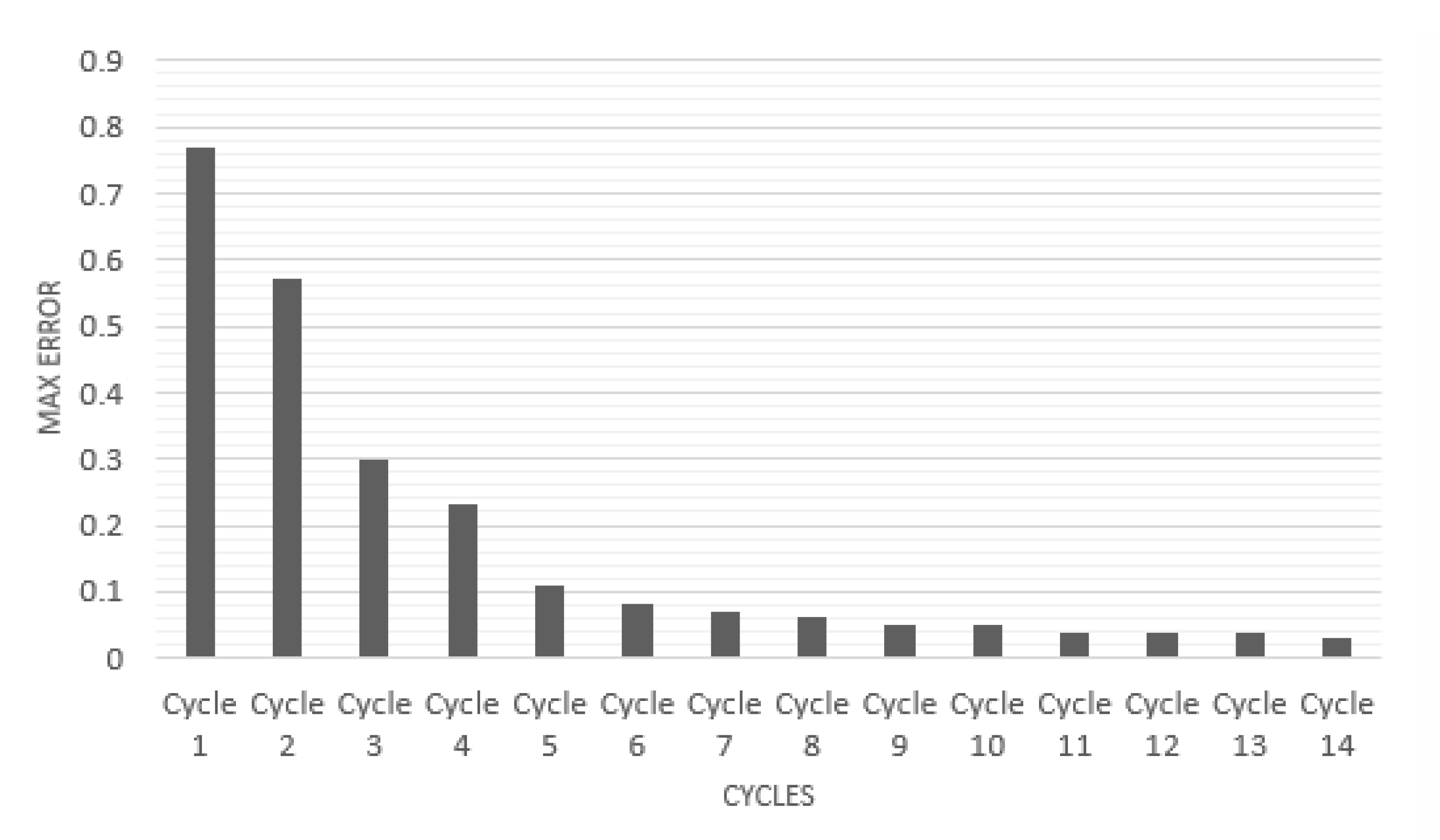
Figure 2 is a graph which empirically shows that the vectors stabilize one cycle after another. Shown in the graph is max$\left(|x_k\left(new\right)-x_k\left(old\right)|\right)$ against cycle number. The maximum is computed over the components of the vector and over all vectors $x_k$. One can observe that after around 15 cycles the changes in vectors become very small, indicating their convergence to their particular positions in the space.

4. Vocabulary and Data Gathering

To design the proposed word embedding, we have collected data in the form of labeled pairs of words from multiple sources. Moreover, we explored the properties of the vocabulary that achieve best results using our algorithm. We model our vocabulary as a graph referred to as the graph of words, such that the words are the vertices and relations between the words are the edges. (graph modeling has been a very useful tool in natural language processing; see [39].) Weights are attached to the edges of the graph, and these weights represent the similarity scores between the two words they each connect. The existence of an edge means that a labeled word pair exists as a part of the vocabulary to train the algorithm. There is, however, a potential problem. The graph could have a number of components that are disconnected from each other; i.e., no sequence of edges can lead from one component to the other. This could lead to potentially multiple solutions for the optimization task. The algorithm would not know where to place the vectors corresponding to the disconnected components with respect to each other. In other words, one can rotate entire connected groups without them affecting the error function (in Equation (1)), because no similarity terms exist between any of the disconnected groups’ vertices. This would lead to arbitrarily estimated similarities between the vectors (words) of any two disconnected components.

Venkatesh p. 124 [40] provides an in depth investigation of when a large graph is void of disconnected components; i.e., one large connected component. He proves the following theorem:

Theorem 2.

Consider a graph with n vertices and with probability p that an edge exists between any two vertices. If $p=\frac{\log n}{n}+\frac{c}{n}$, for some constant c, then the probability that the random graph $G(n,p)$ is connected tends to $e^{-e^{-c}}$, as $n⟶\infty$.

This theorem essentially says that if $p>>\log \left(n\right)/n$ then the graph is one giant connected component. Since the expected degree of each vertex is $k=np$, this means that the average degree of our graph should be generally higher than log(n); i.e., $k>\log \left(n\right)$. We used this fact as a guide in determining the number of synonym/antonym pairs used to create the training set, since each pair will create an edge in the out graph of words.

At the end of generating the training set, we apply the networkx python algorithm [41] to detect the number of components in a graph. There may still be several disconnected components. In such a case, we manually select pairs of words corresponding to the disconnected components. We seek to connect them by estimating the similarity using our judgment of the word meanings. This essentially draws edges between the disconnected components. Ideally, how many edges should we add between any two disconnected components? The answer is d, the dimension of our vector space. This would essentially anchor the vectors in fixed places with respect to each other. It would also prevent the possibility of rotating a component with respect to another along some remaining degrees of freedom without violating the existing distances or similarities between the vectors as given in the training set.

To collect our vocabulary we have used several sources. This is in order not to rely overly on one single source. We used the following:

• Lists for frequent English words’ synonyms and antonyms extracted from the web sites: [42,43].
• Lists for certain categories that we manually constructed; e.g., family, sports, animals, countries, capitals, and others (we added 33 lists). Each list consists of many words, and we assigned a specific similarity score among the words in each list, based on our judgment.
• We collected an extensive amount of words from WordNet [44] and from other sources, such as educational websites and books [45,46,47,48,49,50,51,52,53]. Subsequently, we created a crawler that would visit the site of thesaurus.com (the premier site for word meanings, synonyms, antonyms, etc.) [54]. The crawler would fetch the synonyms and antonyms of the sought words from the thesaurus. The obtained words would be fed again to the site and more synonyms and antonyms were obtained, and so on. These would then be added to the training set.
• We gathered random word pairs from a site that contains random phrases [55]. We checked these pairs, and selected only the ones that were unrelated. As mentioned before, unrelated pairs should give similarity around zero, and they have the important task of connecting disconnected groups in the graph. In addition to the unrelated pairs, we collected synonyms and antonyms for these selected words using the crawler from thesaurus.com.
• We gathered other unrelated word pairs randomly by pairing words manually in the constructed vocabulary (of course after checking that they are indeed unrelated).
• We manually added some synonyms, antonyms, and unrelated word pairs using other different online dictionaries.

For the collected pairs we have assigned a similarity close to 1 for synonyms and close to −1 for antonyms. This is just the theoretical target function. After convergence it typically yields different similarities. The reason is that there is competition between words to pull the vectors of its synonymous words towards its vector. This results in “middle ground” vector locations that satisfy reasonable contiguity towards its different synonyms.

Table 1. Vocabulary structure.

Number of distinct words (graph vertices)	27770
Number of synonymous pairs	102260
Number of antonymous pairs	38783
Number of unrelated pairs	182287
Number of graph edges	323330
Ratio of number of edges to number of vertices	11.64
Average degree of the graph	23.29
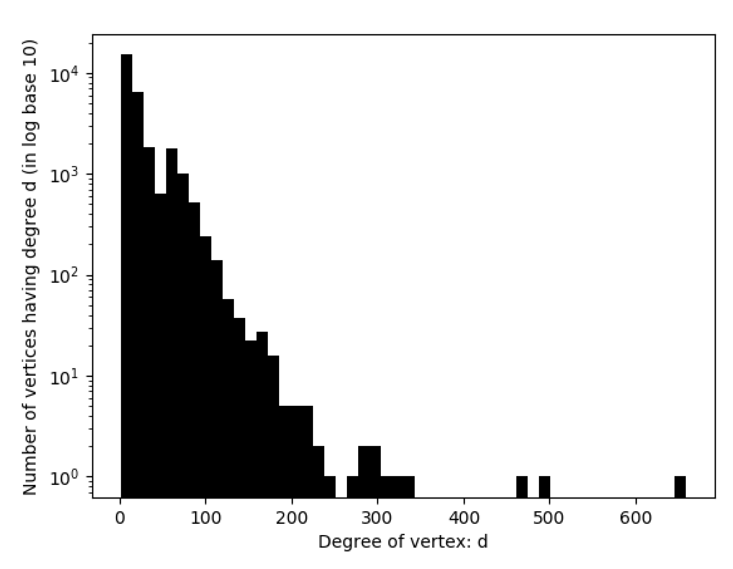
Number of connected components	1

shows the structure of the constructed vocabulary while Figure 3 is a histogram for the degree of vertices in the constructed vocabulary.

5. Results and Discussion

We have tested the proposed word embedding method. After a thorough design, and training using our method, we have performed the following four evaluation experiments in addition to outlining an opinion mining application for hotel reviews:

• Word Similarity: We present the similarity scores obtained between many selected word pairs, and compare with the scores of other published word vector representations. The comparison of the performances should be done using the judgment of the reader.
• Human Judged Similarity: We apply our approach and some competing methods on benchmark word pair lists. These lists, published in some papers, have human-judged similarity scores. So this allows comparison with actual numbers.
• Antonymy Detection: We evaluate our approach on answering closest-opposite questions (extracted from the GRE test), comparing our results with the published ones.
• Antonym/Synonym Discrimination: We test the performance of our approach in discriminating between antonyms and synonyms. The performance is compared with other published word vector representations.
• Opinion Mining: We outline the application of our method on an opinion mining task. Moreover, we use other published word vectors to compare the performance on such task.

All used datasets are the same for all the compared models in order to have fair comparisons. In all the conducted experiments, we used the word vectors generated using our implemented algorithm. The training vocabulary used is the one gathered as explained in the previous section. The generated word vector’s number of dimensions is 50.

5.1. Word Similarity

Table 2. Word similarity comparison (* means the pair is not part of the training set for our method).

Word1	Word2	Sphere (Our Approach)	Word2vec [17]	GloVe [19]	FastText [20]
happy	joyful	0.944	0.424	0.598	0.701
amusing	happy	* 0.778	0.27	0.387	0.5
king	queen	* 0.83	0.651	0.76	0.764
boy	girl	* 0.859	0.854	0.825	0.862
male	female	* 0.702	0.841	0.938	0.945
education	student	0.608	0.401	0.682	0.547
movement	motion	0.887	0.231	0.56	0.583
oscillate	move	* 0.828	0.239	0.166	0.354
district	county	* 0.733	0.594	0.651	0.586
district	commune	0.761	0.164	0.367	0.464
friend	partner	0.96	0.37	0.609	0.619
valuable	worthy	0.849	0.351	0.537	0.649
great	tremendous	0.858	0.775	0.668	0.804
joyfulness	joy	* 0.986	0.513	0.362	N/A
France	Paris	0.94	0.555	0.721	0.632
Germany	Berlin	0.949	0.554	0.685	0.673
Egypt	Cairo	0.934	0.602	0.699	N/A
France	French	0.82	0.633	0.686	0.68
Germany	German	0.801	0.681	0.7	0.742
Egypt	Egyptian	0.869	0.602	0.718	0.753
Japan	China	* 0.738	0.315	0.697	0.645
Japan	Greece	* 0.609	0.545	0.494	0.595
african-country	european-country	* 0.88	N/A	N/A	N/A
modern	ongoing	* 0.487	0.129	0.357	0.424
obsolete	outdated	* 0.915	0.743	0.725	0.797
money	shopping	* 0.599	0.166	0.487	0.407
internet	web	0.888	0.597	0.737	0.683
apple	orange	* 0.93	0.392	0.493	0.561
soccer	football	0.926	0.731	0.819	0.804
lion	tiger	* 0.987	0.512	0.621	0.67
giraffe	animal	0.954	0.422	0.436	0.573
light	sun	* 0.612	0.401	0.525	0.558
geology	earth	* 0.701	0.264	0.444	0.531
tenor	opera	* 0.847	0.459	0.395	0.519
unauthorized	simultaneously	* −0.101	0.175	0.237	0.3
bag	country	* 0.061	0.085	0.301	0.367
beach	truck	* 0.448	0.09	0.296	0.421
array	again	* 0.294	−0.011	0.314	0.317
useful	wash	* 0.195	0.073	0.288	0.224
tourism	beach	* 0.513	0.266	0.389	0.459
decent	morning	* 0.027	0.041	0.373	0.253
go	new	* 0.111	0.113	0.564	0.345
yes	no	−1	0.392	0.695	0.549
active	passive	−0.916	0.436	0.577	0.678
happy	unhappy	−0.912	0.613	0.565	0.767
young	old	−0.841	0.417	0.573	0.583
youth	old	* −0.357	0.212	0.384	0.392
youth	elderly	−0.674	0.215	0.39	0.499
valuable	valueless	* −0.912	0.334	0.262	0.614
recall	forget	* −0.907	0.3	0.532	0.567
education	ignorance	−0.854	0.2	0.306	0.487
complex	easy	* −0.769	0.213	0.439	0.453
beginning	deadline	* −0.73	0.22	0.447	0.348
modern	outdated	* −0.933	0.404	0.427	0.528
unlike	same	* −0.957	0.299	0.681	0.482
grow	eradicate	* −0.858	0.241	0.308	0.491
certainty	uncertainty	−0.931	0.492	0.617	0.706
truth	lying	* −0.766	0.237	0.468	0.479
daring	coward	* −0.676	0.196	0.233	0.432
decelerate	speed	* −0.843	0.212	0.22	0.385

contains a number of word pairs where the corresponding similarity scores are obtained by the proposed word embedding. The similarity score is computed as the dot product between unit vectors. We have compared our scores with the scores of other published pre-trained word vectors: word2vec [17], GloVe [19], and fastText [20]. The number of dimensions of the vectors in word2vec, GloVe, and fastText is 300, while the dimension of the vectors in our approach is 50. The reason for selecting a number of dimensions of 50 is that more dimensions lead to sparser space, and more overfitting. N/A means that one or both of the words in the given pair have no pre-trained vectors in the method considered. In the table we have included word pairs from different categories:

• Synonyms that occur in the training vocabulary of the proposed method.
• Synonyms that are not part of the training vocabulary of the proposed method (marked with the * symbol in the table).
• Antonyms that are part of the training vocabulary.
• Antonyms that are not included as part of the training vocabulary (also marked with the * symbol).
• Unrelated words that occur in the training vocabulary.
• Unrelated words that are not part of the training vocabulary (marked with the * symbol).
• Word pairs that belong to a certain category (e.g., countries).

Note that the pairs that are not part of the training set constitute an unbiased out of sample test, since the algorithm has not seen them while training.

From Table 2, we can observe several interesting facts:

• By human judgment, the proposed algorithm seems to be more successful in capturing the similarity between the different words. For example, the pairs “happy–joyful”, “amusing–happy” and “district–county” are close synonyms, and our algorithm manages to assign a high similarity. Opposing algorithms give low similarity scores around 0.5 or so.
• For the antonyms, our algorithm assigns rightly negative numbers. For example, the pairs “modern–outdated” and “unlike–same” are assigned similarities lower than −0.8. The competing algorithms assign similarities in the range of about 0.3 to 0.68, not really signaling that these words are antonyms.
• For unrelated words, the proposed embedding generally gives them similarities close to zero. For example, the pairs “array–again”, “useful–wash” and “decent–morning” are given respectively 0.294, 0.195, and 0.027, which are reasonably close to zero.
• The competing algorithms are not very successful in differentiating antonyms from unrelated pairs. They give them all comparable scores. For example, the antonyms “modern–outdated” and “unlike–same”, and the unrelated pairs “array–again”, “useful–wash” and “decent–morning” are given similarities in the same range. It is not clear from the scores whether the pair is an an antonym or an unrelated pair. Additionally the pair “yes–no” is the most basic antonym, and in spite of that, the competing algorithms do not give them a zero score.
• An antonymous pair such as “happy–unhappy” is given a high similarity score in all the other three competing approaches. Thus it is treated the same as a synonymous pair while it is given a negative similarity score in our approach.
• An antonymous pair such as “decelerate–speed” is given a low similarity score in all the other three approaches, and thus is treated the same as an unrelated pair while it is given a negative similarity score in our approach.
• In all the four approaches, the “country–capital” pairs have close similarities.
• In all the four approaches, the “country–nationality” pairs have close similarities.
• The pair “Japan–Greece” has a lower similarity score than the pair “Japan–China”, although both pairs are country pairs. This is due to the fact that Japan and China have more properties in common (both are Asian countries, and are distance-wise close to each other).
• A combination such as “African-country” is not found in any of the other three vocabularies. Since the other approaches do not represent such composite words as vectors.
• We must caution, however, that the competing methods word2vec, GloVe, and fastText are not specifically designed to handle antonyms. Therefore, the comparison presented, which shows clear domination of our method for antonyms, may not be fully due to a particular design or algorithmic outperformance, but also partly due to the fact that the competing methods were not designed to deal with antonyms.

5.2. Human Judged Similarity

We considered here datasets from other researchers that attached human-judged similarity scores to the word pairs. This would give an unbiased assessment, as the similarity estimate is performed by different researchers. None of the human-judged similarity scores associated with the pairs in these datasets are included in our training set, in order to have it as an out of sample test.

We considered the labeled data of MC30 [56] and RG [57], which have human-judged similarity measures. There is a third dataset available, namely, the WordSim-353 [58] human-judged dataset, but we did not perform a test using this dataset because they estimated antonyms as similar while in our approach we consider antonyms as opposites. We computed two metrics, the Spearman rank correlation (Sp) and root mean square error (RMSE). Moreover, we have compared the obtained metrics’ values with those of word2vec [17], GloVe [19], and fastText [20].

Table 3. Results of human-judged datasets.

Approach	MC30		RG
	Sp	RMSE	Sp	RMSE
Sphere (our approach)	0.91	0.18	0.9	0.15
word2vec	0.8	0.3	0.76	0.29
GloVe	0.79	0.27	0.82	0.25
fastText	0.83	0.24	0.84	0.22

shows that we achieve the best results for both metrics on both datasets.

5.3. Antonymy Detection

We have applied our approach on answering the closest-opposite GRE questions, collected in [27,30]. The GRE, or Graduate Record Examinations, is a worldwide exam needed for admission to graduate schools. The verbal part has a group of multiple choice questions that seek the closest-opposite. The 162 questions of the development set are used as a part of our training vocabulary; i.e., the words together with the correct answers are added to the training vocabulary as antonymous pairs. On the other hand, both the 950 questions and the 790 questions datasets are used as test sets (i.e., their pairs do not exist in our training set).

We applied our word embedding method to compute the similarities between the word in question and all candidate answers, and selected the answer that is closest to −1, signifying an antonym. We have computed the precision, recall, and F-score as given in [27], so that we could make comparisons with the numbers given in the competing methods. They are given by

$$Precision\left(P\right)={\displaystyle \frac{\mathrm{Number}\mathrm{of}\mathrm{questions}\mathrm{answered}\mathrm{correctly}}{\mathrm{Number}\mathrm{of}\mathrm{questions}\mathrm{attempted}}}$$

(14)

$$Recall\left(R\right)={\displaystyle \frac{\mathrm{Number}\mathrm{of}\mathrm{questions}\mathrm{answered}\mathrm{correctly}}{\mathrm{Total}\mathrm{number}\mathrm{of}\mathrm{questions}}}$$

(15)

$$F-score={\displaystyle \frac{2\times P\times R}{P+R}}$$

(16)

In our case we note that the precision = recall = F-score; this is because our approach attempted all the questions. All the words that exist in the questions and in the candidate answers have corresponding vectors in our word embedding method.

Furthermore, we compared our results with the best results recorded in [27,29,30,31,32,34] that use the same dataset. From

Table 4. Results of closest-opposite GRE.

Approach	Development Set			Test Set 950			Test Set 790
	Precision	Recall	F-Score	Precision	Recall	F-Score	Precision	Recall	F-Score
Sphere (our approach)	0.98	0.98	0.98	0.83	0.83	0.83	0.8	0.8	0.8
Mohammad et al., 2008 [27]	0.76	0.66	0.70	0.76	0.64	0.70	-	-	-
Yih et al., 2012 [29]	0.88	0.87	0.87	0.81	0.80	0.81	-	-	-
Mohammad et al., 2013 [30]	0.79	0.66	0.72	-	-	-	0.77	0.63	0.69
Chang et al., 2013 [31]	0.88	0.85	0.87	0.81	0.77	0.79	-	-	-
Zhang et al., 2014 [32]	0.88	0.88	0.88	0.82	0.82	0.82	-	-	-
Ono et al., 2015 [34]	0.92	0.91	0.91	0.90	0.88	0.89	0.89	0.87	0.88

, it is shown that we achieved the best precision, recall, and F-score for the development set. We achieved the second best scores in both test sets after [34]; however, the dimension of their vectors is 300 while the dimension of our vectors is only 50. As mentioned earlier, their model is trained such that there is no differentiation between antonymous pairs and unrelated pairs, as both will have low similarity scores. Moreover, we were able to compare our results with [34] only on antonymy detection as the authors did not include the performance of their vectors on synonyms or unrelated words.

5.4. Antonym/Synonym Discrimination

In this section, we show using statistical measures how our approach perform in the task of discriminating between antonyms and synonyms. Moreover, our approach’s performance is compared to the other published word vectors’ models: word2vec [17], GloVe [19], and fastText [20]. The used dataset is introduced by [35]. This dataset considers word pairs in three categories: adjectives, nouns and verbs. The pairs are marked as antonyms or synonyms. Therefore, we have conducted this experiment as a binary classification task with two classes namely, antonyms and synonyms. The classification is done based on the similarity score between the vectors of the word pair. If this similarity score is equal to or greater than a certain threshold (more specifically 0.5), then the pair is classified as synonyms otherwise the pair is classified as antonyms. The used dataset is refined such that pairs that have any non-existent word in any of the models are removed. After this refinement the dataset has the following structure:

• 470 adjectives: (238 antonyms and 232 synonyms);
• 547 nouns: (276 antonyms and 271 synonyms);
• 632 verbs: (311 antonyms and 321 synonyms).

In

Table 5. Antonym/synonym discrimination results—adjectives.

Approach	Precision	Recall	F-Score	Accuracy
Sphere (our approach)	0.86	0.83	0.83	82.98%
word2vec	0.61	0.56	0.50	55.96%
GloVe	0.65	0.60	0.57	60.43%
fastText	0.67	0.67	0.67	66.81%

,

Table 6. Antonym/synonym discrimination results—nouns.

Approach	Precision	Recall	F-Score	Accuracy
Sphere (our approach)	0.72	0.72	0.72	72.39%
word2vec	0.65	0.58	0.51	57.77%
GloVe	0.67	0.62	0.58	61.61%
fastText	0.67	0.66	0.65	65.81%

and

Table 7. Antonym/synonym discrimination results—verbs.

Approach	Precision	Recall	F-Score	Accuracy
Sphere (our approach)	0.83	0.81	0.81	81.49%
word2vec	0.70	0.54	0.43	53.80%
GloVe	0.69	0.59	0.53	59.02%
fastText	0.66	0.63	0.61	62.66%

the performance measures are recorded for the four models and for the three categories respectively. The results show that our model outperforms all the other three models in all the categories.

5.5. Comments on the Results

We can observe that the proposed word embedding approach gives more reasonable similarity scores than some of the major approaches, such as word2vec, GloVe, and fastText. These methods have a particular deficit dealing with antonyms, and distinguishing between antonyms and unrelated words. The failure of some of them in assigning the right similarity score to the pair “yes” and “no” is case in point. Our algorithm also fared better on the two benchmarks tested. It also did well compared to other algorithms that are specifically designed to deal with antonyms, on the GRE antonym dataset. Furthermore, our approach proved its efficiency in discriminating between antonyms and synonyms as compared to other published word vectors’ models. Our algorithm can handle composite words (like “fairy tale”). It could potentially also handle words with multiple meanings, such as “bat” (the animal) and “bat” (a club). The way to tackle these is to consider them as different words, like “bat-1” and “bat-2”. The challenge facing all word embedding methods is to distinguish words with multiple meanings from the context of the sentence.

5.6. Opinion Mining

Opinion mining application refers to classifying a review as positive or negative. We applied our approach to learn vectors for words that have bias from which sentiments can be inferred. We have begun with a small set of such words then grow our sphere by obtaining synonyms and antonyms for these words. The generated word vectors are used to compute the sentiment that the review reflects. Every word in the review has two sub-scores that are obtained by respectively the dot product between this word and a number of positive words on one hand, and a number of negative words on the other hand, which are specifically collected to gauge sentiment. We applied the approach to 20,000 hotel reviews [59] from “515K Hotel Reviews Data in Europe” dataset [60] that are collected from booking.com where each review is annotated as positive or negative. Furthermore, we used vectors from other models to compare the results. We achieved the highest F-score compared to word2vec [17], GloVe [19], and fastText [20]. The scores obtained are 0.81, 0.79, 0.74, and 0.79 respectively [61].

6. Conclusions

In this work we have devised a new approach for embedding words into a sphere. The algorithm is a simple relaxation one without the need for intensive training phases. The approach is a polarity capturing one in the sense that antonymous word pairs are located at opposite poles of the sphere. Not only antonymy can be detected but also other relations (e.g., unrelated pairs).

We have managed to gather an adequate vocabulary that can flexibly be extended. Moreover, we evaluated our approach using several datasets, showing that the approach competes well with other approaches in the literature. We have successfully proved that our approach does not suffer from the ambiguity in differentiating between various word pair relations such as synonyms, antonyms, and unrelated pairs.