Abstract
Diffusive surfaces are considered as one of the most challenging aspects to deal with in the acoustic design of concert halls. However, the acoustic effects that these surface locations have on the objective acoustic parameters and on sound perception have not yet been fully understood. Therefore, the effects of these surfaces on the acoustic design parameters have been investigated in a real shoebox concert hall with variable acoustics (Espace de Projection, IRCAM, Paris, France). Acoustic measurements have been carried out in six hall configurations by varying the location of the diffusive surfaces over the front, mid, and rear part of the lateral walls, while the other surfaces have been maintained absorptive or reflective. Moreover, two reference conditions, that is, fully absorptive and reflective boundaries of the hall have been tested. Measurements have been carried out at different positions in the hall, using an artificial head and an array of omnidirectional microphones. Conventional ISO 3382 objective acoustic parameters have been evaluated in all conditions. The results showed that the values of these parameters do not vary significantly with the diffusive surface location. Moreover, a subjective investigation performed by using the ABX method with auralizations at two listening positions revealed that listeners are not sensitive to the diffusive surface location variations even when front-rear asymmetric conditions are compared. However, some of them reported perceived differences relying on reverberance, coloration, and spaciousness.
1. Introduction
The definition of materials for absorptive and diffusive surfaces is the main design issue once the shape and the volume of an auditoria have been determined. These surfaces can be used by acousticians and architects to reach the desired sound field and achieve a trade-off with the aesthetical architectural aspects [1]. In performance spaces, the absorptive surfaces are usually hidden by layers of perforated panels or textiles. Conversely, the diffusive surfaces are commonly visible and become an important part of the design of the interior space. Their effects have been intensively investigated in the last decade and are usually related to corrections of the acoustic glare, echoes, focusing of sound, and enhancement of the uniformity of the sound field [1,2,3]. Depending on the combination with the absorptive surfaces, they can also generate negative effects, such as the reduction of sound level and reverberation time [4]. Diffusive surfaces are considered one of the most critical aspects in the acoustic design and renovation of concert halls since there is a lack of knowledge on how their effects on the sound field are related to practical design choices, that is, their location and extension. Thus, this experimental study aims to give more insight on the former aspect, by investigating the effects of diffusive surface location on the objective acoustic parameters used in the design process. Moreover, the sensitivity of listeners to variations in the diffusive surfaces location is investigated.
It has been highlighted that the direct relation between the diffusive surfaces and any objective acoustic parameter is not as immediate as the absorptive surfaces related to the reverberation time [5]. Therefore, more adequate diffuser design and evaluation tools for acousticians and architects are needed since the preliminary phases of the design process to promote the use of sound diffusers. In order to better understand the diffusive surfaces effects, several case studies have been used for objective and subjective investigations through measurements in real halls [4,6,7,8], physical-scale models [4,8,9,10,11,12], and simulations of performance spaces [12,13,14,15,16].
Different investigations have focused on the ISO 3382-1 [17] parameters since these are used as design parameters at a larger scale. Ryu and Jeon [4] found that hemispherical and polygonal diffusers installed on the sidewalls close to the proscenium arch, the sidewalls of stalls, and balcony fronts of a shoebox-horseshoe plan hall decrease sound pressure level (SPL), reverberation time (RT) and early decay time (EDT) at most seats, compared to reflective surfaces. Furthermore, these surfaces affect clarity (C80) and the interaural cross-correlation coefficient (1-IACCE) by increasing and decreasing their values at the front and the rear seats, respectively. Other investigations on the effects of hemispherical diffusers applied to 1:50 scaled rectangular and fan-shaped hall surfaces confirmed the decreasing effects of diffusers on RT and SPL [9]. In this study, the halves of the lateral walls closest to the stage have been judged as the most effective areas for diffuser installation since they reduce the spatial deviation of the acoustic parameters and minimize the decrease of RT and listening level (LL). This was mainly valid for shoebox halls rather than fan-shaped halls. Moreover, large and sparse diffuser profiles resulted as more effective on the acoustic results. Jeon et al. [18] made measurements in real reverse fan-shaped and rectangular halls and found that saw-tooth and cubic shaped diffusers installed on lateral walls do not have any significant effect on the acoustic parameters. However, their presence improves the spatial uniformity of the sound energy. Based on simulations in a fan-shaped hall with two different hall volumes (3600 m3 and 7300 m3), Shtrepi et al. [16] showed that the ISO 3382 objective parameters are mostly affected when the diffusive surfaces with a scattering coefficient higher than 0.70 are located on the ceiling, lateral walls and rear wall simultaneously. These effects are more evident in the smaller volume and are reduced when the rear wall only is treated independently of the volume. Jeon et al. [19] have suggested the use of another objective parameter, namely the number of reflection peaks (Np) in an impulse response, which describes the spatial and temporal variation of the sound field. They considered a scaled model of a shoebox hall with polygon- and hemisphere-type diffusive surfaces applied to the lateral walls and ceiling, as well as a real reverse fan-shaped recital hall with diffusive front halves lateral walls closest to the stage. Their measurements showed an increase in the Np at higher frequency bands and no significant differences for the other ISO 3382 parameters. In addition, Jeon et al. [12] showed differences below the just noticeable difference (JND) for the ISO acoustic parameters through simulations in 12 performance halls of various shapes (shoebox, fan-shape, and other complex shapes) and with increasing scattering coefficient of the walls and ceiling. In a second part of the study based on measurements in a scale model of a vineyard-shape hall, they noticed that the periodic diffusers installed over the sidewalls and balcony decrease RT and G (strength), while increase C80. However, this was mainly attributed to the absorption added by the diffusers.
Besides the objective investigations, also the perceptual differences between different surface treatments have been the object of continuous research. Torres et al. [20] showed that changes in diffusion characteristics of the surfaces are audible in a wide frequency region and depend on the input signals, i.e., sustained signals make the perception of the differences easier than impulsive signals. Takahashi and Takahashi [21] and Shtrepi et al. [7] showed that perceptual differences between reflective and diffusive surfaces are related to the listening distance from the surface itself. Moreover, they are related to the difference of scattering coefficient between the compared surfaces [13,15]. Singh et al. [22] found that the perceived diffuseness is related to the interaural cross-correlation coefficient (IACC), which is an important parameter in the design process. Furthermore, Jeon et al. [19] showed that the perceived diffuseness could be quantified in terms of the number of reflected peaks (Np), which is correlated to the listener preference. In another study, Ryu and Jeon [4] showed that the preference of the diffusive surface presence highly correlates with the perceived loudness (SPL) and reverberance (EDT). Other studies reported that changes in diffusive surfaces characteristics are mainly perceived in terms of coloration and spaciousness variations [7,20,21,23]. Jeon et al. [12] showed that despite small changes in the objective parameters, the presence of the diffusers made a clear and positive contribution to the overall impression of the listeners, which was mainly related to intimacy and envelopment.
Although these results highlight the importance of the location of the diffusive surfaces and their configuration combined to the size and shape of the hall, there is still need for clear and generalized guidelines useful for acousticians and practitioners alike. Since the scattering properties of these surfaces can be easily assessed by using the ISO 17497-1, -2 [24,25], the application of diffusive surfaces based on scientific investigations, and not only on the architectural and design preferences, should be a common practice for modern concert hall designers. Moreover, the subjective data, i.e., the listeners’ sensitivity, would help to determine the measurement accuracy needed for the characterization of these surfaces [26].
However, very little research on this aspect has been carried out in real concert halls due to both technical and economic issues. Therefore, the present study attempts to clarify the influence of diffusive surface location on the objective and subjective aspects by means of both in-situ measurements and perceptual listening tests. Since both technical and economic issues would limit the research, a flexible environment—the hall Espace de Projection at IRCAM (Paris)—has been involved. Six configurations have been created by varying the location of the diffusive surfaces over the front, mid and rear part of the lateral walls, while the other surfaces have been maintained absorptive or reflective. Moreover, two reference conditions, that is, fully absorptive and reflective boundaries of the hall have been tested. The ISO 3382 objective acoustic parameters, such as reverberation time (T30), early decay time (EDT), clarity (C80), definition (D50), center time (Ts), and interaural cross-correlation (IACC) have been estimated from the measured impulse responses. Furthermore, subjective investigations have been performed in order to identify the detectable differences between different locations of the diffusive surfaces.
2. Method
2.1. Objective Measurements
2.1.1. Hall Description
A variable-acoustic environment, the Espace de Projection (ESPRO) at IRCAM in Paris (Figure 1), has been used for in-field measurements in order to investigate how the location of diffusive surfaces can influence the generated sound field. Table 1 provides the architectural and acoustical details of the variability of ESPRO based on Peutz [27,28]. The hall characteristics have been extensively described in Shtrepi et al. [7,13,14] and here only a brief overview is given in order to help the reader understand the context of the experiment.

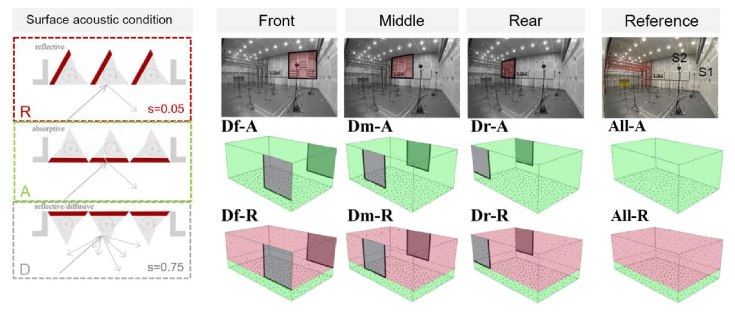
Figure 1.
Surface acoustic conditions absorptive, reflective, and diffusive (A, R, and D). Interior view and simplified models of the eight configurations of the hall. Six configurations tested with three different locations of the diffusive surfaces (Df-A, Dm-A, Dr-A, Df-R, Dm-R, Dr-R) and two reference conditions (All-A and All-R).

Table 1.
Architectural and acoustical details of the ESPRO based on Peutz [27,28].
The ESPRO is a modern facility with variable passive acoustics, which is achieved through the variation of room geometry and surface acoustic properties: the former is reached by moving the ceiling height from 3.5 m up to 10 m, while the latter is controlled by acting on independently pivoting prisms. The prisms are grouped in panels of three and have three faces with different acoustic properties that are reflective, diffusive, and absorptive (Figure 1). The frequency-dependent absorptive and scattering properties of the surfaces have been shown in [7], while diffusion polar distributions have been presented in [13,14]. Based on these references, the data at 500–1000 Hz for the absorptive surfaces present a mean absorption coefficient of a = 0.80, while the diffusive surfaces are characterized by a mean scattering coefficient of s = 0.75 and a diffusion coefficient of d45° = 0.52. The rotation is automated and managed from a control room. Only the eye-level panels, i.e., the first row from the floor level, are controlled manually and could be set in either absorptive or reflective conditions. The floor is a hard-reflective surface.
2.1.2. Hall Acoustic Conditions and Measurements
Six hall configurations have been considered in this study by varying the location of the diffusive surfaces over the lateral walls within two different main acoustic conditions of the overall surfaces of the hall: absorptive (-A) and reflective (-R) (Figure 1). Three conditions of the diffusive surfaces (Figure 1 and Figure 2) have been tested by shifting their location over the front, mid, and rear part of each lateral wall (hereafter labeled Df, Dm, Dr, respectively). Moreover, two reference conditions, that is, all variable surfaces set in the absorptive (All-A) and reflective (All-R) mode have been considered in order to investigate the overall absolute effect of the presence of a diffusive surface.
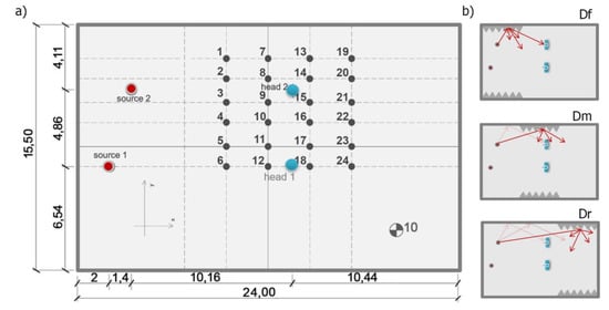
Figure 2.
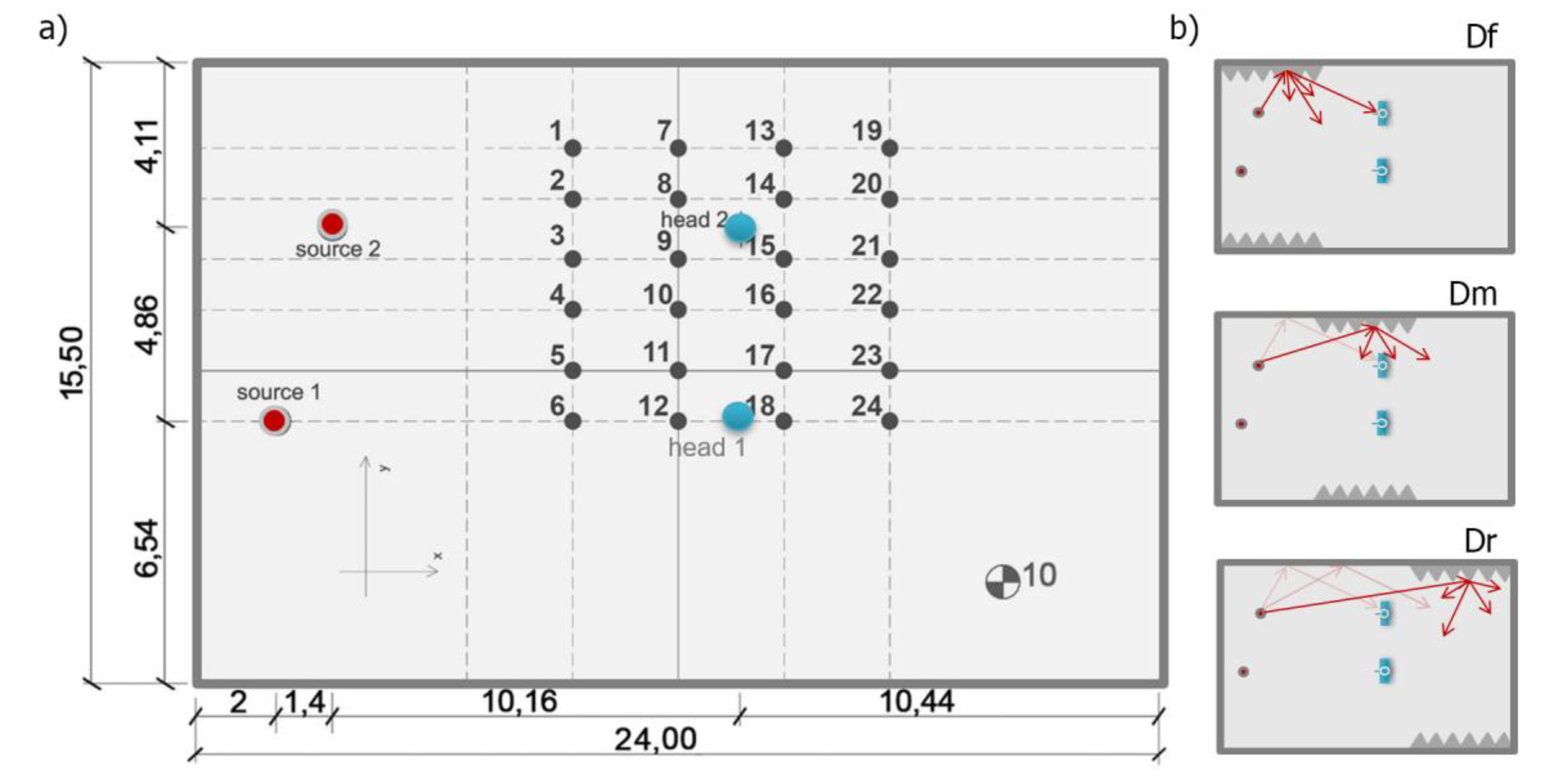
(a) Measurement positions (source, microphones, and artificial head) and main dimensions of the room (metric scale). (b) Schematic plan view of the diffusers location with respect to the source and artificial head positions.
The absorptive condition was chosen for the eye-level fixed panels in all the measurements in order to avoid the strong reflections from the lower parts of the walls. The ceiling was set at the maximum operative height of 10 m, i.e., leading to a room volume of 3720 m3.
ISO 3382-1 [17] objective parameters have been measured in the unoccupied room conditions. A detailed description of the measurement set-up is given in [7], while here a brief overview is given in order to help the reader understand the main elements. Measurements have been carried out using the ITA-Toolbox, an open-source toolbox for Matlab [29]. Monaural and binaural measurements have been performed with twenty-four omnidirectional microphones (Sennheiser KE-4) and two artificial heads (ITA Head), respectively (Figure 2). The microphones have been set at a height of 3.7 m in a crossed array that extended to one of the two halves of the audience area (Figure 1 and Figure 2). This height was chosen in order to reach the center of the first level of variable panels. Additionally, the artificial heads (Head 1 and Head 2) have been placed in the middle of the microphone array in order to be representative of the largest number of receiver positions and adjusted at an ear height of 3.7 m from the floor level as the omnidirectional microphones. Head 1 was located close to the central symmetry axis of the room and Head 2 at the midway between the axis and the lateral wall. The impulse responses at these positions have been used for the auralization introduced in the listening test session. Two omnidirectional sound sources have been positioned at the front part of the room. Each source consisted of a three-way system of low, medium, and high-frequency sources, which were positioned at different heights, that is, at 0.40, 3.70, and 3.90 m, respectively [7]. The excitation signal was an exponential sine sweep with a sampling rate of 44.1 kHz, a length of 16.8 s, and a frequency range separated for each speaker of the sources. Two repetitions have been performed for each configuration; however, given the high S/N ratio no averaging was applied [30]. Three Octamic II by RME (Haimhausen, Germany) have been used as microphone preamps and an ADA8000 Ultragain Pro-8 by Behringer (Willich, Germany) served as DA-converter. Loudspeaker, artificial head, and amplifier were custom made devices by the Institute of Technical Acoustics, Aachen, Germany.
2.1.3. Objective Analyses
The ISO 3382-1 [17] parameters, that is, reverberation time (T30), early decay time (EDT), clarity (C80), definition (D50), center time (Ts), interaural cross-correlation (IACC) have been assessed by using the functions of ITA-Toolbox. Specifically, these parameters have been considered as a measure of reverberance and liveness (T30 and EDT), clarity and balance between early and late energy, or the balance between clarity and reverberance (C80, D50, and Ts), and perceived spaciousness (IACC). This last parameter has been evaluated only for the binaural measurements at the head locations.
Averaged values, as suggested in ISO 3382-1 [17], have been calculated over the 500 Hz and 1000 Hz octave bands, while the IACC values were averaged over 500 Hz, 1000 Hz and 2000 Hz octave band results since these frequencies concern the subjectively most important range. Besides the IACC for the full length of the impulse responses, the early-arriving (0–80 ms) and late-arriving (80 ms-inf) sound have been considered separately in the evaluation of IACCE and IACCL, respectively. The JND values of each parameter have been used to compare the results for different configurations (Table 2).
Table 2.
Objective acoustic parameters and respective JND values.
2.2. Subjective Investigation
An auditory experiment has been conducted to investigate the listener’s ability to perceive variations of the diffusive surfaces location by using the ABX method [31]. The test also allowed to evaluate the effects of different source and listener positions and type of music/signal passages (Figure 3).
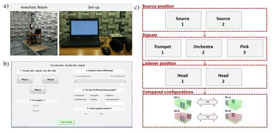
Figure 3.
(a) Listening test anechoic room set-up, (b) user-interface in Italian, and (c) listening test scheme.
2.2.1. Test Subjects and Experimental Environment
A group of twenty-four professors, research assistants, and students aged between 25 to 50 years old with normal hearing ability have been involved in the test. All the listeners were volunteers interested in acoustic topics and no one of them could be considered as an expert listener, based on their musical experience. All of them provided written consent for the anonymized use of their test results. The normal hearing ability of each listener was tested by using the app “Loud Clear Hearing Test,” developed by JPSB Software [32] and the same headphones (Sennheiser 600 HD) subsequently used in the listening test. This procedure is helpful for a more accurate screening compared to just self-reported hearing ability, which is often used in acoustic investigations.
The listening test sessions have been conducted in the anechoic room at Politecnico di Torino (Figure 3a), which has a background noise of LAeq = 17.3 dB. During the two days test, the room conditions, as well as the set-up, have been kept unvaried. The equipment consisted of one computer, a sound card (Tascam US-144 MKII), and headphones (Sennheiser 600 HD). The environment was made comfortable for the listeners and they were familiarized with the test procedure by an illustrated written and verbal explanation.
2.2.2. ABX Method
The ABX methodology [31] is a standard psychoacoustic test for the determination of audible differences between two signals. In this procedure, three stimuli are presented to the listener: stimulus “A” and stimulus “B,” which have a known difference, and stimulus “X”, which regards the task of the listener who has to identify whether it is the same as “A” or the same as “B.” If there is no audible difference between the two signals, the listener’s responses should be binomially distributed such that the probability of replying “X = A” is equal to the probability of replying “X = B,” i.e., 50%. This score is interpreted as indicating no perceptual difference between A and B. The minimum number of correct answers needed to indicate a perceptual difference can be given by the inverse cumulative probability of a binomial distribution, based on the number of trials, confidence level and probability of correct answer.
For the sake of this investigation, an ad-hoc routine in Matlab 2018b (MathWorks, Natick, MA, USA) with an intuitive user interface in Italian language has been implemented to present the test to each participant (Figure 3b).
2.2.3. Test Procedure
The listening test consisted of signals recorded in the same “head” position (Figure 1), i.e., Head 1 and Head 2 for the front-rear asymmetric configurations (Df-A, Dr-A, Df-R, and Dr-R). Figure 3c depicts the test structure. A pair of two different configurations are compared in each experiment (Df-A vs. Dr-A or Df-R vs. Dr-R), while the sources, the artificial head, and the music/signal passage remain unvaried within each pair of samples.
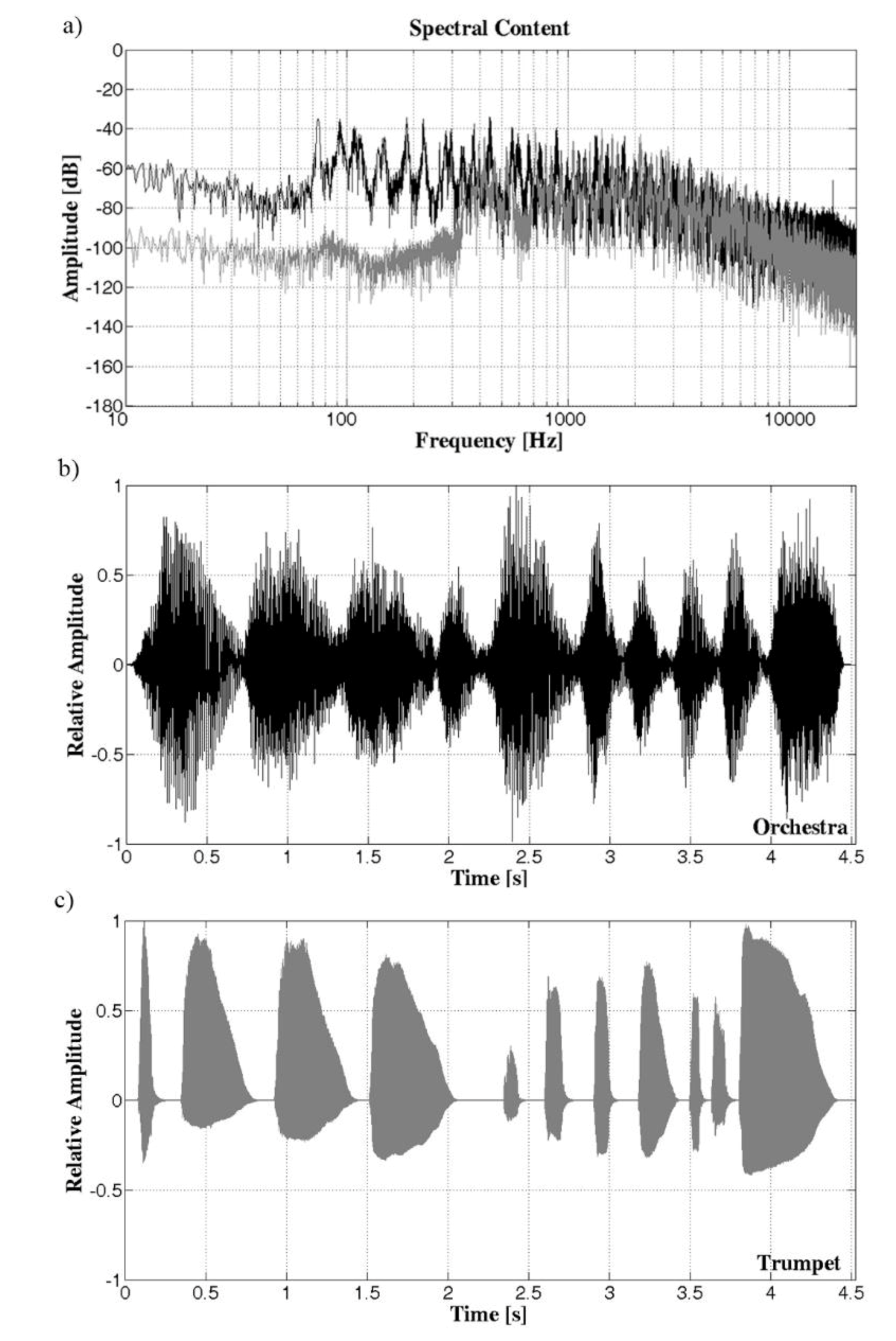
The auditory tests consisted of 48 stimuli (24 pairs), which were created by convolving the binaural impulse responses obtained from in-situ measurements with three anechoic music passages. The three music/signal passages were chosen based on different style, tempo, and spectral contents: an orchestra track (“Water Music Suite”—Handel/Harty, Osaka Philarmonic Orchestra, Anechoic Orchestral Music Recordings, Denon, Kawasaki, Japan), a solo instrument trumpet (MAHLER_tr1_21.wav, Mahler, Odeon anechoic signals database) and pink noise. The temporal and spectral contents of the first two samples are shown in Figure 4. The pink noise was included in the test for its objective and perceptual acoustic properties, although it is not a realistic signal for concert halls. Pink noise has a well-known spectral density that decreases at a rate of 6 dB per octave which leads, on average, to the same amount of power for every octave band. From a perceptual point of view, the signal sounds flatter to the ear. The orchestra and trumpet signals present some differences below 400 Hz, where the trumpet sample has less energy (Figure 4a). Figure 4b,c shows the temporal development and the characteristics of the transients in the signals. The trumpet sample is constituted by abrupt onsets and reasonably damped offsets, while the orchestra sample is a more sustained signal that has ramped onsets and damped offsets. The listening test samples are made available in an open-access repository [33].

Figure 4.
Orchestra and trumpet anechoic stimuli: (a) spectral content, (b) waveform of the orchestra sample, and (c) waveform of the trumpet sample.
A sample length of 5 s was chosen to be long enough in order to give the listener the necessary time to assess the full extent of their acoustic perception and, at the same time, short enough to avoid excessive fatigue. Given the comparative structure of the test, no equalization has been applied for the sound level between the conditions in each pair.
The test was structured as a double-blind test, i.e., the administrator did not know the answers either, in order to avoid any accidental cues to the listeners. Moreover, the test was based on a fully randomized order of presentation of A and B pairs, as well as a random distribution of the correct answers, i.e., X could be randomly A or B. After listening to A and B, the listeners were asked to answer to the question “Which one is X?” by choosing between one of three options, that is, “sample A” and “sample B.”
Compulsorily, the listeners had to listen to all of the three samples (A, B, and X) in order to continue to the next step of the test. However, they could freely choose the listening order of the three samples (A, B, and X) and repeat the samples as many times as they judged necessary.
The listeners did not receive any instructions on which features of the sound samples they should concentrate on. This aspect was investigated (Figure 3b) by asking them to give more details on their answers related to:
- “How strong is the difference?” The answer was given on a 0–10 scale.
- “What kind of difference could you perceive?” The answer was given by selecting the relevant attributes (coloration, spaciousness, clarity, reverberance, and loudness) that have been perceived as different. Listeners could choose more than one option or indicate other unincluded attributes.
- “Which signal do you prefer?” The answer was given by choosing between A and B.
The authors explained the case study and the purpose of the experiment at the end of the individual test. The listeners could not take breaks during the test, which lasted about 30 min. After the test, the listener’s impressions and opinion were collected. Further information was gathered on their experience with previous listening tests, on their music skills, as well as on their age and general health conditions.
3. Results
3.1. Objective Results
Figure 5, Figure 6, Figure 7, Figure 8 and Figure 9 show the results of each objective room acoustic parameter in all the considered hall conditions. Each parameter is given with respect to the source-to-receiver distance (S1 and S2). Moreover, the figures provide the objective acoustic parameter differences between the configurations Df-Dm, Df-Dr, Dm-Dr for an easier direct comparison to the JND values for the absorptive (-A) and reflective (-R) conditions, respectively. Differences within ±1 JND of the parameters are highlighted through a gray area. A summary of these differences has been given numerically in the tables in Appendix A.
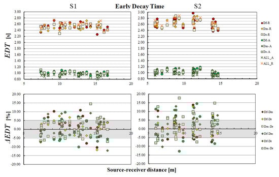
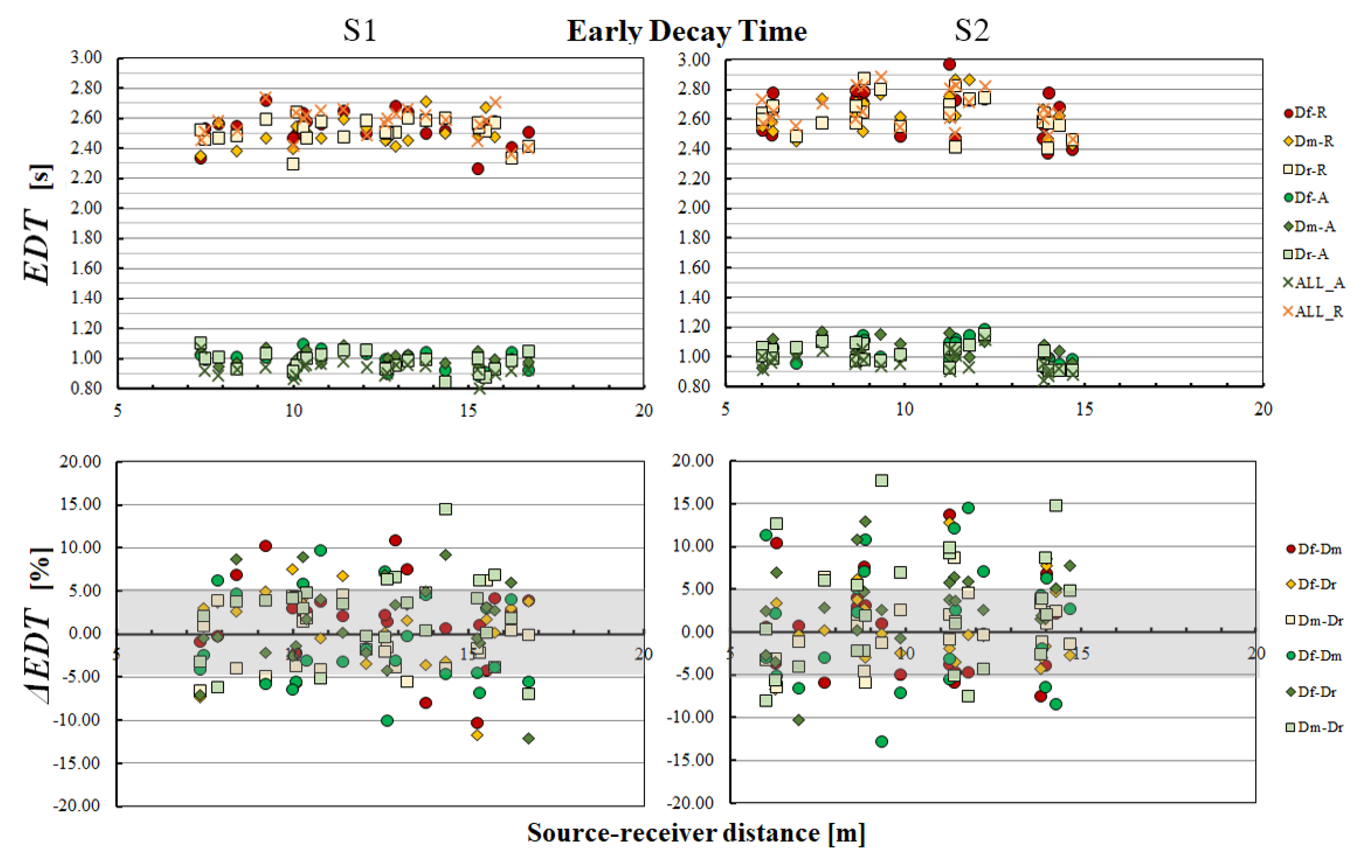
Figure 5.
EDT parameter averaged over 500 Hz and 1000 Hz for S1 and S2 source-to-receiver distance. ΔEDT represents the parameter differences between the configurations Df-Dm, Df-Dr, Dm-Dr in the reflective (-R) and absorptive (-A) conditions. Differences equal ±1 JND of the parameters are highlighted through a gray area.
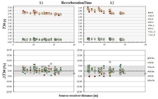
Figure 6.
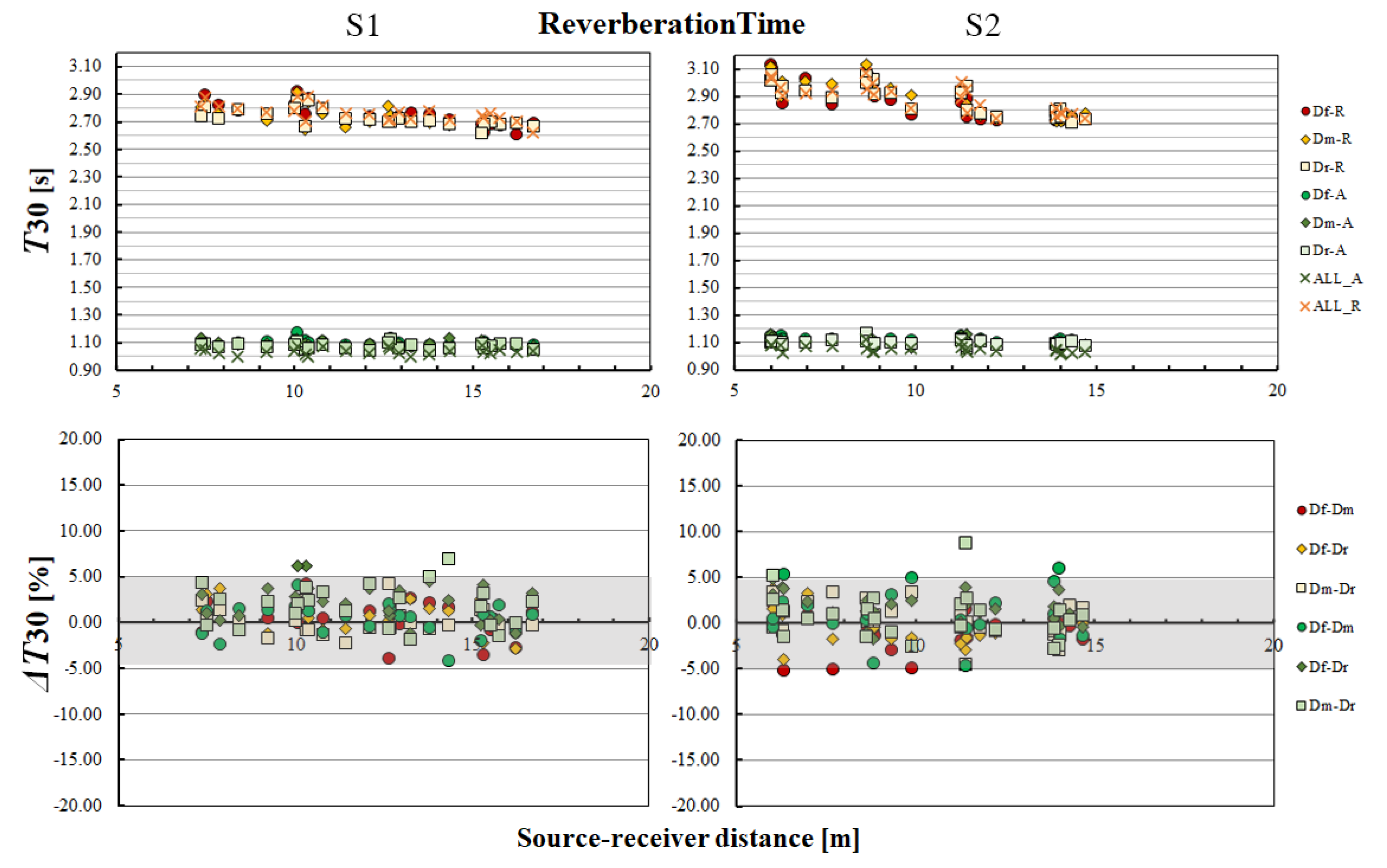
T30 parameter averaged over 500 Hz and 1000 Hz for S1 and S2 source-to-receiver distance. ΔT30 represent the parameter differences between the configurations Df-Dm, Df-Dr, Dm-Dr in the reflective (-R) and absorptive (-A) conditions. Differences equal ±1 JND of the parameters are highlighted through a gray area.
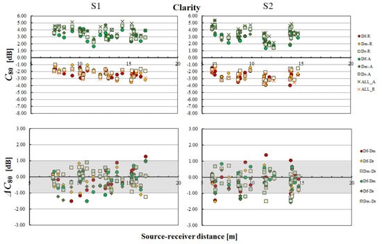
Figure 7.
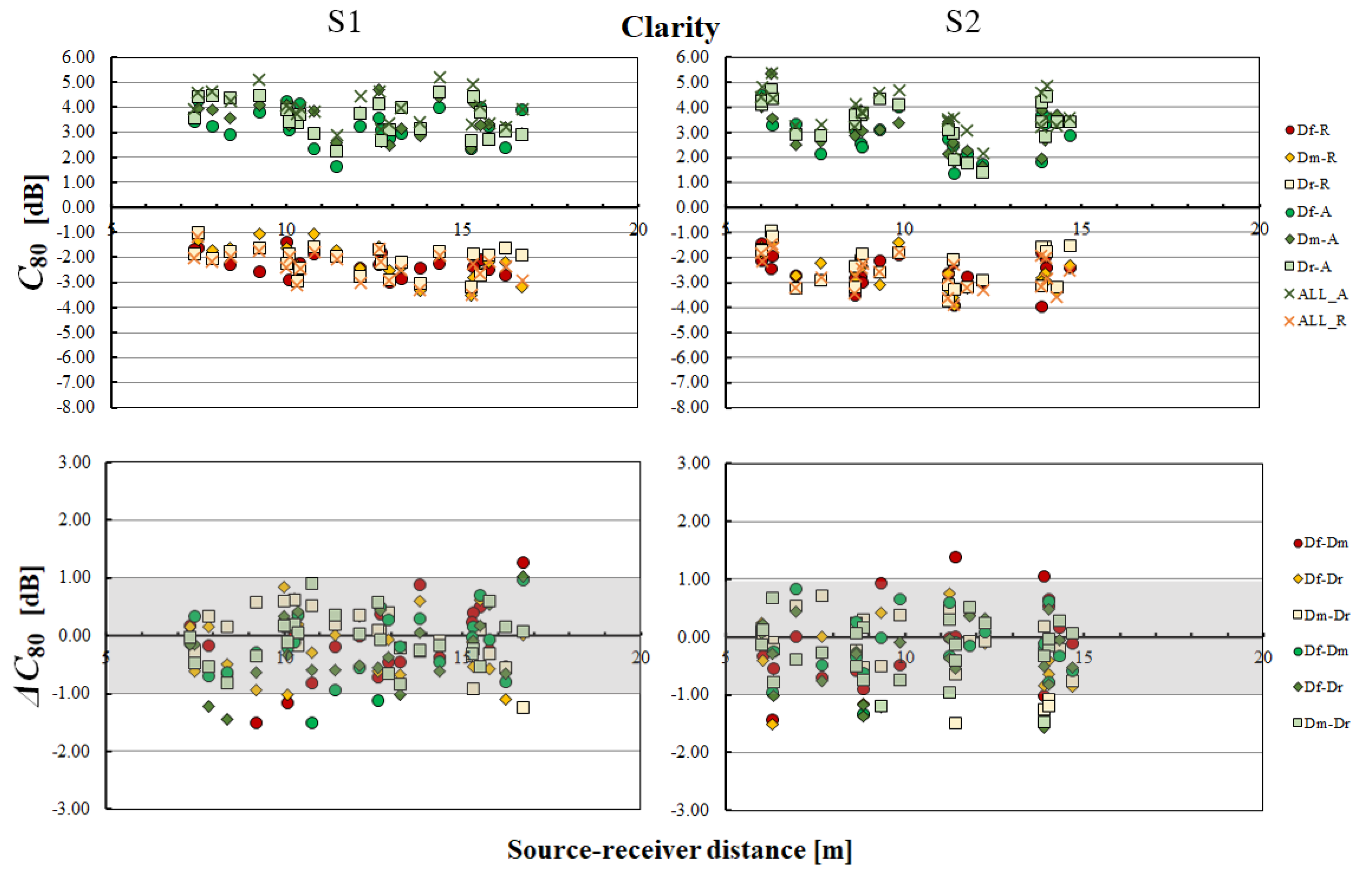
C80 parameter averaged over 500 Hz and 1000 Hz for S1 and S2 source-to-receiver distance. ΔC80 represents the parameter differences between the configurations Df-Dm, Df-Dr, Dm-Dr in the reflective (-R) and absorptive (-A) conditions. Differences equal ±1 JND of the parameters are highlighted through a gray area.
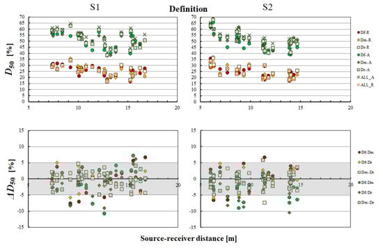
Figure 8.
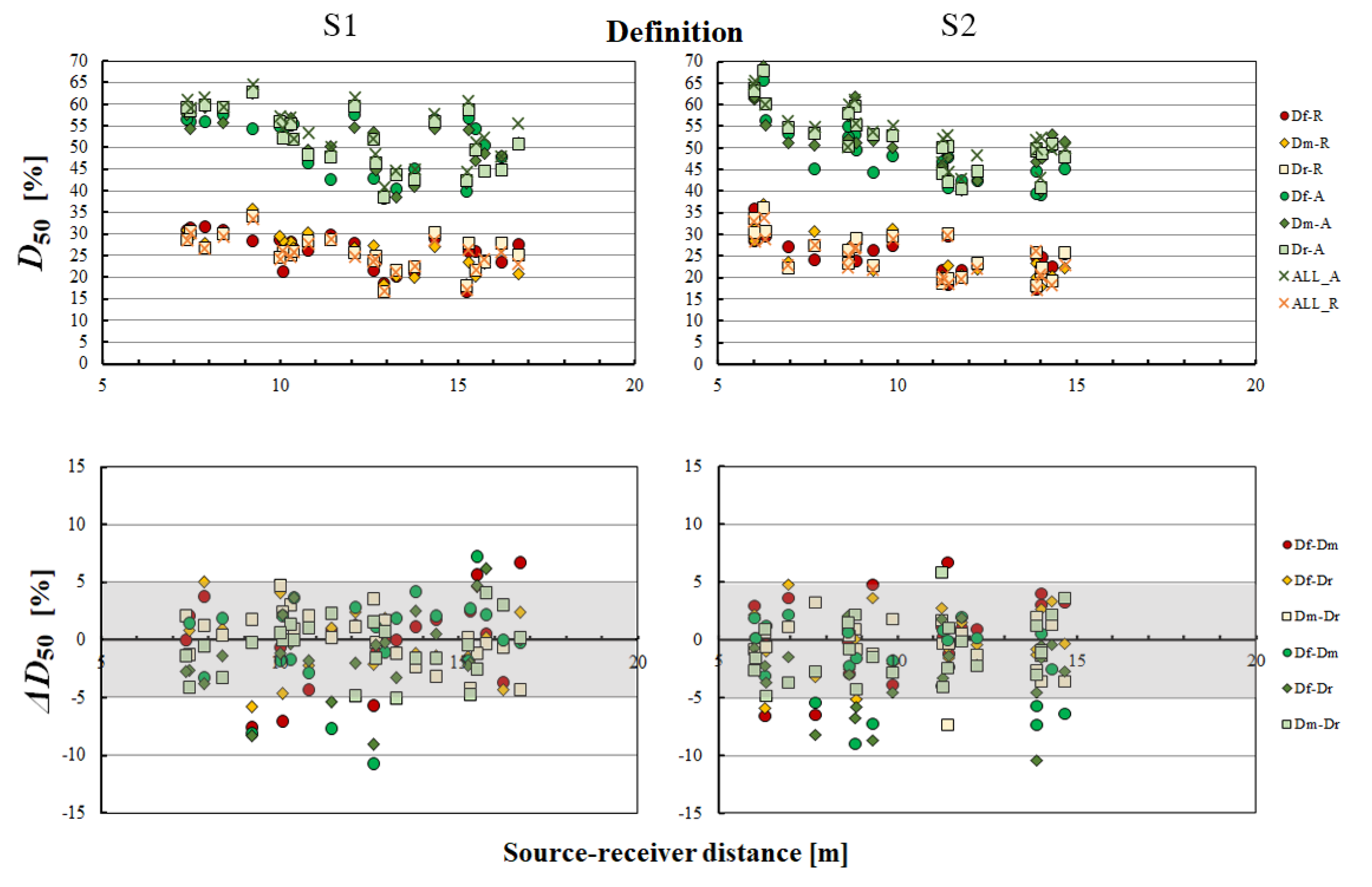
D50 parameter averaged over 500 Hz and 1000 Hz for S1 and S2 source-to-receiver distance. ΔD50 represents the parameter differences between the configurations Df-Dm, Df-Dr, Dm-Dr in the reflective (-R) and absorptive (-A) conditions. Differences equal ±1 JND of the parameters are highlighted through a gray area.
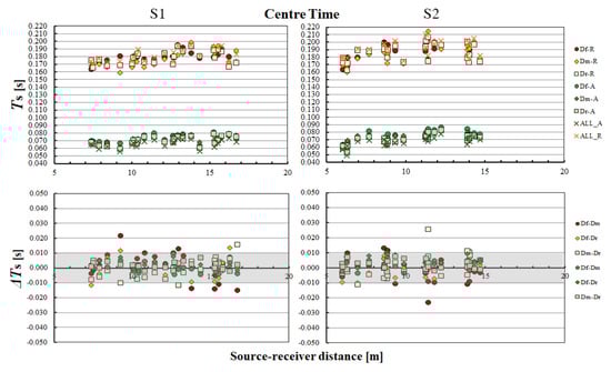
Figure 9.
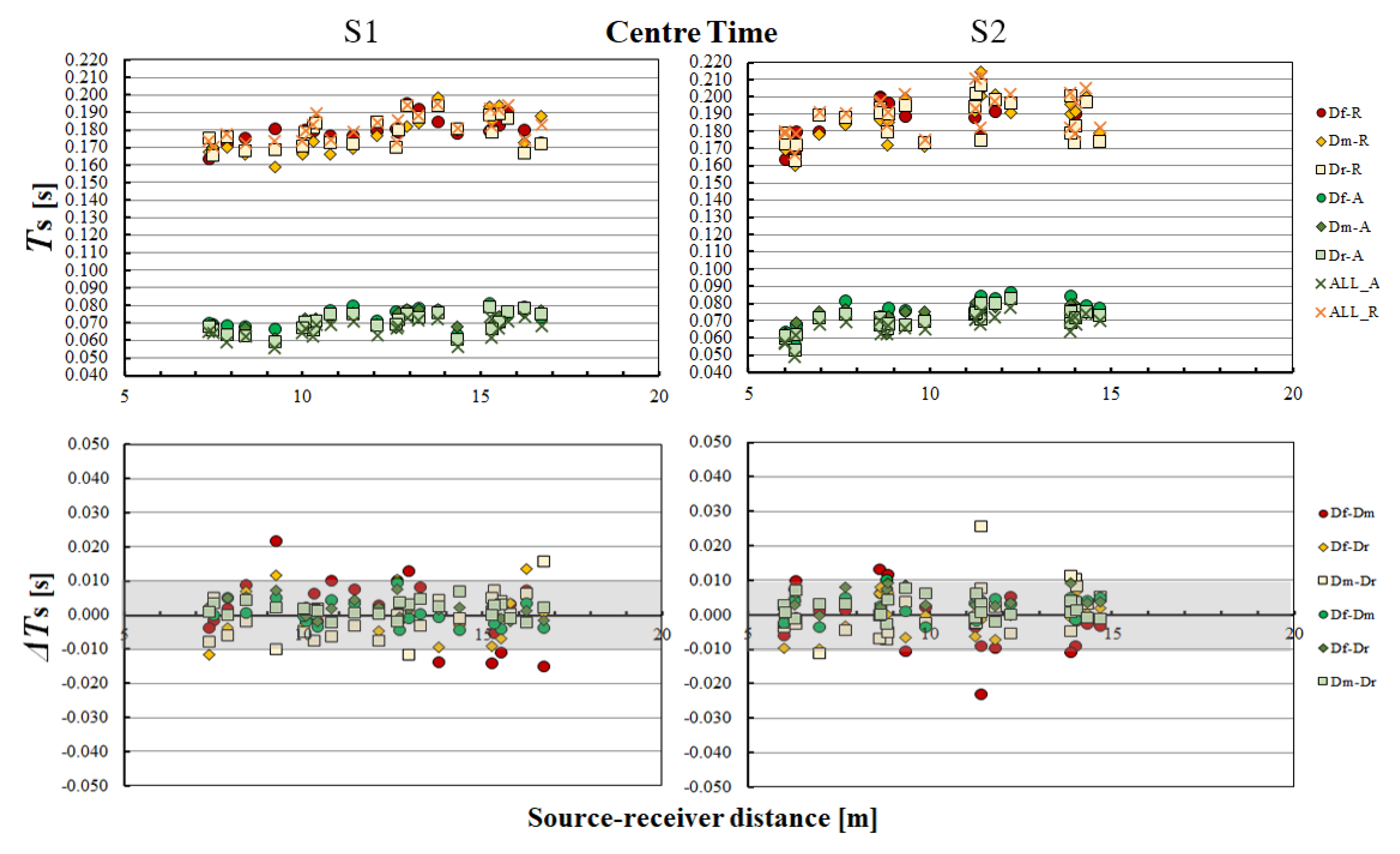
Ts averaged over 500 Hz and 1000 Hz for S1 and S2 source-to-receiver distance. ΔTs represent the parameter differences between the configurations Df-Dm, Df-Dr, Dm-Dr in the reflective (-R) and absorptive (-A) conditions. Differences equal ±1 JND of the parameters are highlighted through a gray area.
The results of EDT (Figure 5) do not show a strong dependence on the source-to-receiver distance for both S1 and S2 in both the reflective (-R) and absorptive (-A) conditions. EDT values of the reflective conditions result higher for source location S2 compared to S1 for source-to-receiver distances between 8–12 m. The ΔEDT graph shows that there are a few significant differences between the configurations Df-Dm, Df-Dr, Dm-Dr in the reflective (-R) and absorptive (-A) conditions, i.e., >1 JND. These differences result higher for source location S2 and occur at a larger number of receivers in the absorptive (-A) conditions. However, no significant trend could be observed with respect to the source-to-receiver distance.
The results of T30 (Figure 6) show a decrease at the farthest positions for both S1 and S2 in the reflective conditions Df-R, Dm-R, Dr-R, and All-R. Conversely, there is no decreasing trend in the absorptive conditions Df-A, Dm-A, Dr-A, and All-A. T30 values of the reflective conditions result higher for source location S2 compared to S1 for the nearest receivers. Very few receiver locations seem to present differences (ΔT30) higher than the JND between the different diffuser locations Df-Dm, Df-Dr, Dm-Dr in the reflective (-R) and absorptive (-A) conditions. However, no significant trend can be detected considering the overall receivers and the source-to-receiver distance.
The results of C80 (Figure 7) present different trends for S1 and S2 with respect to the source-to-receiver distance in both the reflective (-R) and absorptive (-A) conditions. Generally, it can be noticed that ΔC80 values present a few differences higher than the JND between the different diffuser locations Df-Dm, Df-Dr, Dm-Dr in the reflective (-R) and absorptive (-A) conditions. However, it not possible to detect a significant general trend of differences due to the diffuser location when a comparison is made overall the source-to-receiver distances.
The results of D50 (Figure 8) show a decrease at the farthest positions both for S1 and S2 in the reflective (-R) and absorptive (-A) conditions. It can be noticed that D50 values present a higher variability in the absorptive conditions at each receiver position for both sources. Generally, it can be noticed that ΔD50 values present a few differences higher than the JND between the different diffuser locations Df-Dm, Df-Dr, Dm-Dr in the reflective (-R) and absorptive (-A) conditions. However, no significant trend can be detected considering the overall receivers.
The results of Ts (Figure 9) show an increase at the most distant positions both for S1 and S2 in the reflective (-R) and absorptive (-A) conditions. Only a very few receiver locations seem to present differences higher than the JND between the different diffuser locations. This is observed mainly for the reflective (-R) conditions.
A statistical analysis has been performed on the data shown in Appendix A to investigate the main factor (that is the absorptive/reflective conditions, source S1 and S2, source-to-receiver distance) effects on the variability of the objective acoustic parameters in the comparisons between the tested configurations (Df-Dm, Df-Dr, Dm-Dr). To this aim, only differences above the JND have been considered since it is not meaningful from an acoustic point of view to investigate data lower than the perceived ones. Thus, EDT, which resulted in the most affected parameter, was retained suitable for a statistical analysis given the relatively high number of receiver locations that showed differences above the JND. However, it was not possible to apply an ANOVA analysis since the assumptions of normality of data distribution and homogeneity of variance are violated. Given this result, the Kruskal–Wallis (KW) test, which is a non-parametric test and an extension of the Mann–Whitney U Test for more than two groups, has been applied [34]. The Kruskal–Wallis test did not show a statistically significant result (p > 0.05) for the differences due to the diffusers location variations.
Table 3 shows the differences in the spatial mean values of each parameter obtained in the conditions with the three different locations of the diffusive surfaces (Df, Dm, and Dr) with respect to the absorptive (All-A) and reflective (All-R) conditions. It can be noticed that the overall results show significant differences for the EDT in all the configurations (Df, Dm, and Dr) and also for T30 in the Df and Dm configurations with respect to All-A. However, this might be due to the variation of the equivalent absorption area, which decreases when one part of the lateral absorptive walls is set into a diffusive condition. This effect is not evident with respect to the reflective condition (All-R).
Table 3.
Spatial mean values and overall standard deviation of reverberation time (T30), early decay time (EDT), clarity (C80), definition (D50), center time (Ts) in the eight conditions. Differences (Δ = All − D) with respect to the reference configurations All-A and All-R are given in brackets for each configuration (Df, Dm, and Dr). The differences above the JND have been highlighted in bold.
A more detailed analysis of the objective parameters has been performed at the head positions. Table 4 gathers the differences of the objective parameters between each compared pair for source position S1 and S2 in the subjective test. The objective parameters at the head position have been evaluated as the values of the parameters obtained at the nearest microphone positions, i.e., microphone position 18 for head 1 and average values of microphone positions 14 and 15 for head 2. The conditions Df and Dr, i.e., the subjectively compared conditions, that lead to differences between the objective parameters above the JND are highlighted in bold.
Table 4.
Objective acoustic parameters obtained at the head position for the compared pairs of configurations. The differences above the JND between Df and Dr values in the reflective (-R) and absorptive (-A) conditions have been highlighted in bold.
The combination of the listening position head 1 and source location S1 presents a greater number of parameters (EDT, D50, and IACCL) that reveal differences above the JND in the comparison of Df-A towards Dr-A. Conversely, in the reflective condition (-R), significant differences (>JND) are present only for Ts values. No significant differences can be observed for the combination of the listening position head 2 and source location S1 in both the reflective (-R) and absorptive (-A) conditions.
The combination of the listening position head 2 and source location S2 presents significant differences (>JND) for EDT only in both conditions (-R and -A). No significant differences can be observed for the combination of the listening position head 1 and source location S2 in both reflective (-R) and absorptive (-A) conditions.
3.2. Subjective Results
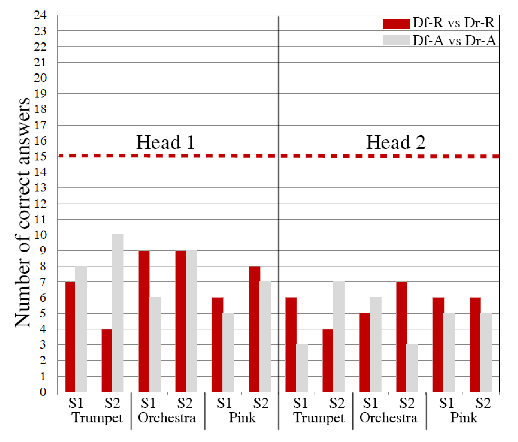
The subjective data gathered from the listening tests have been analyzed based on binomial distribution [35] in order to determine the statistical significance of the test results. The inverse cumulative probability is used to evaluate the minimum number of correct answers that are needed to indicate a perceptual difference. The inverse cumulative probability is given as a function of the trials (corresponding to the thirty-one listeners), probability of correct answers (50%), and confidence level (95%). Therefore, the minimum number of correct answers necessary to indicate a significant difference between pairs at a 95% confidence level was found to be 15, i.e., correct answers should result equal or higher than 15.
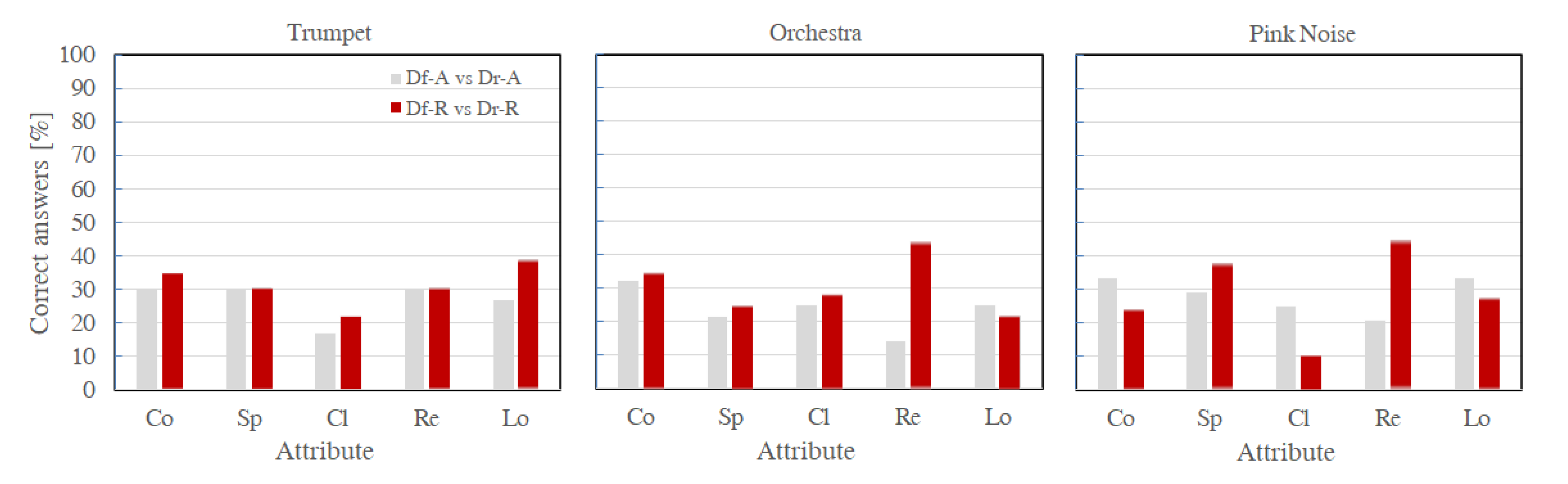
Figure 10 shows the correct answers for each music/signal passage, listening (head), and source position. The dashed horizontal line indicates the minimum number of correct answers necessary to detect a significant perceptual difference between configurations compared in one pair. No significant variations of the location of diffusive surfaces were significantly perceived in any of the compared pairs. Some of the listeners could still indicate a few differences relying on different attributes as presented in Figure 11, which shows the occurrences of each attribute given in the correct answers. Further, according to the feedback of the listeners, for each signal (trumpet, orchestra, pink noise), more than 75% of the correct answers were given by relying on two or more attributes (reverberance, coloration, and spaciousness). Among them, reverberance is the main attribute when the orchestra and pink noise samples are compared in the reflective condition.

Figure 10.
Listening test results. The dashed horizontal line indicates the minimum number of correct answers necessary to indicate a significant perceptual difference between configurations compared in one pair. x-axis indicates the pairs compared in each trial.
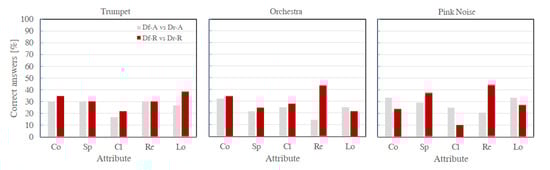
Figure 11.
Listening test results. The listeners’ subjective evaluations on the perceived differences between front and rear location of the diffusive surfaces in the absorptive and reflective conditions (Df-A vs. Dr-A and Df-R vs. Dr-R). The y-axis depicts the occurrences of each attribute given in the correct answers. The x-axis reports the attributes Co—coloration, Sp—spaciousness, Cl—clarity, Re—reverberance, Lo—loudness.
Finally, given the small perceived differences, it was not possible to collect reliable results regarding the preference indicated by the listeners.
4. Discussion
This work aims to give more insight into the design aspects of concert halls related to the effects of diffusive surfaces location. Based on the results presented above, a few practically relevant comments can be made in order to achieve a more mindful design of concert halls and intervene in those areas that could lead to the required objective and perceived acoustic quality.
The objective analyses presented in Figure 5, Figure 6, Figure 7, Figure 8 and Figure 9 and Appendix A showed that the objective parameters are not significantly influenced by the diffusive surface location. These results confirm the findings of previous investigations Jeon et al. [18] and Jeon et al. [12], i.e., the diffusers installation on lateral walls do not have any significant effect on the overall acoustic parameters. However, a few significant differences could be observed at single receiver positions. Generally, no clear trend can be observed for T30, C80, D50, and Ts variations in the different configurations in both the absorptive (-A) and reflective (-R) conditions. EDT was shown to be the most affected parameter. The differences over the configurations show that this is more evident for source location S2 and occurs at a larger number of receivers in the absorptive (-A) conditions. However, no significant trend could be observed with respect to the source-to-receiver distance and the statistical analysis did not show a statistically significant difference between the different diffusers locations. Generally, when the different configurations have been compared to the reference conditions (Table 3), no significant differences resulted in the reflective condition while in the absorptive conditions EDT and T30 resulted in the most affected.
It was shown that in the absorptive conditions (-A), the combination of the listening position head 1 and source location S1 presented a greater number of parameters (EDT, D50, and IACCL) that reveal differences above 1 JND in comparison to Df-A with Dr-A (Table 4). Conversely, the listening position head 2 and source location S2 presented significant differences (>1 JND) for EDT only in both the reflective (-R) and absorptive (-A) conditions. Given these differences, as in previous studies [7,12], it was not possible to correlate the objective parameters differences in these two positions to the perceived differences.
The subjective test did not show significant perceived differences between the configurations Df-A and Dr-A or Df-R and Dr-R, i.e., front-rear asymmetric conditions of the diffusive surface location with respect to the listener position. Some of the listeners could still indicate a few differences by relying on different attributes as presented in Figure 10, which shows the occurrences of each attribute given in the correct answers. However, it was not possible to identify the preferred location of the diffusers due to the small perceived differences. It was observed that for each signal (trumpet, orchestra, pink noise), more than 75% of the correct answers were given relying on two or more attributes (reverberance, coloration, and spaciousness). These attributes have been also highlighted as the most affected in previous studies [4,7,20,21,23]. Reverberance seems to be the main attribute when the orchestra and pink noise samples are compared in the reflective condition. However, despite the differences between the samples typologies it was not possible to determine a significant difference between them, which is in line with the findings in [12,13,14,15,16].
The objective and subjective results highlight the need for further investigations on new parameters. More systematic investigations might focus on the number of peaks (Np) proposed by [19], which correlates to the listener preference or the ‘effective duration’ of the autocorrelation function (τe), which correlates to the intimacy and reverberance [36] and has been proposed as key factor to ‘preferred’ values of several room criteria in relation to different kind of music signals [37].
It should be highlighted that this study focuses on perceptual differences within a shoebox hall only. Different results might be expected for different hall’s shapes and volumes [12,16].
Further research could be performed, as indicated in Kim et al. [9] and Jeon et al. [19], also by taking into account the diffuser shape, size, and directivity of the polar distributions of diffuse reflections. In the ESPRO hall, the diffusers are alternatively vertically or horizontally oriented, i.e., a uniform directivity might be approximated. As it was shown in [9] large and sparse diffuser profiles might result in more effectivity over the acoustic parameters. Moreover, the extension over other surfaces might lead to more significant differences [16]. From the designers’ perspective become more interesting the configurations that do not lead to any significant variation on the objective parameters and on the subjective perception. In this way, there might be more freedom on the aesthetical choices that can be applied to the design of a concert hall once that the acoustic optimal conditions have been obtained.
Limitations of the Study
Given the conditions studied in this paper, it should be noted that the receiver’s area could be extended also at closer or further locations from the source positions. However, given the small spatial variability of the measured objective parameters, we would expect a limited effect also in the very rear part of the hall. The overall number of measurements in this project was made in an automatized way: the surfaces of the room were varied from a control room and the overall set-up of sources and microphone positions were set in the most representative locations in order to avoid entering the room with the risk of variation of its conditions. Therefore, in the attempt to reach the right tradeoff between the gathered acoustic information, room configurations, number of microphones and sources, and time limitations on the use of the room itself, it was concluded that the presented protocol was the most suitable one.
The results of this study have highlighted some important issues related to the relevance of the diffuser’s location in a performance hall. However, it should be underlined that only two listening positions have been used in this investigation. Given the differences that might occur due to source-receiver locations, it might be useful to increase the number of listening positions in order to have clearer evidence of the diffusive surface effects on the overall sound field perception. It might be useful to investigate also more representative positions of the front and rear rows of listeners. However, given the time limitations of the use of the ESPRO for this project, it was not possible to extend the number of dummy head positions. It should be considered that the simplification introduced by an ensemble generated from a single source location on the stage might have influenced the spatial impression for the orchestra sample. When technical and budget availability may cover important experimental costs, multiple sources might be a more accurate representation for this case as shown for the orchestra of loudspeakers in [38,39]. Moreover, in each receiver position, a multi-microphone technique could be used to enable multichannel 3D sound reproduction. Therefore, a spatial sound reproduction could have led to a more realistic listening condition. It might have been easier to identify differences when head movements are allowed since they are naturally used when attending concerts [40].
One of the limitations of this study is related to the use of non-individual HRTF, which could have affected the performance of the subject by diminishing the effects of the different surface locations. Research on the use of individual HRTF data sets has shown that their use would allow for better performance of the subjects in localization tasks and lower front-back confusions [41]. It was not possible to apply individual HRTFs due to the amount of technical effort that should be put to measure these data sets [42]. However, since the same dummy head was used in all the measurements here, this could not have any influence on the relative differences between the compared conditions.
The reverberation time characteristics of around 1 s in the absorptive conditions might have influenced the perception and preference of music samples, which are usually played in rooms with longer reverberation times for optimal listening. However, since the test was based on relative comparisons the influence on the distinction of the differences. Based on the JND definition, it measures the sensitivity of the listeners to a change in a given parameter and is focused on acoustic conditions typically found in concert halls or auditoria [1]. In very large or very small rooms the relations between the different parameters may change and consequently, the perceived differences may also be affected [43]. Therefore, the effects investigated in this research should be considered valid for the room volume of the case study and related ranges of reverberation time.
These aspects remain open to future research where also investigations with experts might lead to a more detailed description of other attributes related to the acoustic quality [44]. Although, previous studies on diffusive-to-reflective surface discrimination have shown compatible results between experts and non-expert listeners [7]. Moreover, also the effects of the diffuser location over the stage area and musicians’ perception could be investigated with specific protocols as in [8]. The effect of diffusers on a different type of performances and related preference remains a crucial point to be further investigated given the importance of the specific effects recreated by the artists’ work [45].
Finally, this study is by no means comprehensive, many other diffusive surface locations strategies exist, and further investigations of additional strategies will be useful to refine and expand the findings presented here over a larger number of hall’s shapes and volumes.
5. Conclusions
In situ measurements and perceptual listening tests have been used to investigate the influence of diffusive surface location on the acoustic parameters used in the design process of concert halls and on the perceived acoustic sound field. The case study involved a real concert hall with variable acoustics (ESPRO, IRCAM, Paris, France), where eight hall configurations have been generated by modifying the characteristics of the lateral walls. The objective evaluation has been carried out by analyzing the variation of the ISO 3382-1 [17] acoustic parameters T30, EDT, C80, D50, and IACC in each configuration, while the perceptual tests have been performed using the ABX method in order to determine whether listeners are sensitive to variations of diffusive surface location. This study gives further insight into the importance of the quantification of the trade-off between the design effort and objective and subjective efficacy of the diffusers application in shoebox halls.
The main conclusions can be summarized as follows:
- The objective parameters are not significantly influenced by the diffusive surface location. No clear trend can be observed for T30, C80, D50, and Ts variations in the different configurations in both the absorptive (-A) and reflective (-R) conditions. EDT results as the most affected parameter.
- The perceived differences between the front-rear asymmetric conditions of the diffusive surface location with respect to the listener position do not show significant differences. However, some of the listeners could still indicate a few differences relying on two or more attributes (reverberance, coloration, and spaciousness). Reverberance seems to be the main attribute when the orchestra and pink noise samples are compared in the reflective condition.
Future work should include different hall shapes and volumes in order to have also a more generalized overview of the interaction between room shape and effects of diffusive surfaces. More effort should be put into the investigation of differently shaped surfaces, i.e., different diffusion patterns and scattering values, and different degrees of diffusive surface extensions. More adequate sound sources and reproduction systems might be used in order to have more accurate results although the technical and economical effort for these improvements seems to be important.
The findings of this study should be seen as a milestone based on in situ results towards the redaction of reliable guidelines, which could enable an easier design process for architects and practitioners alike. The limited effects of the diffusive surfaces give space to a broad field of design alternatives from the designers’ perspective. In this way, there might be more freedom on the aesthetical choices that can be applied to the design of a concert hall once that the acoustic optimal conditions have been obtained. It might be useful to investigate the boundaries of this filed within which the dialog between designers and acousticians would promote further aspects related to creativity.
Author Contributions
L.S. and A.A. conceived and designed the data collection campaigns; L.S. collected data on site; L.S. and S.D.B. performed data analysis; L.S. drafted and curated the first version of the manuscript. All the authors revised the paper. All authors have read and agreed to the published version of the manuscript.
Funding
This research was funded through a Ph.D. scholarship awarded to the first author by the Politecnico di Torino (Turin, Italy).
Acknowledgments
The authors would like to thank all the participants in the listening test sessions for the collaboration. They would also like to express their gratitude to Michael Vorländer, Sönke Pelzer, Renzo Vitale, and Fabian Knauber from the Institute of Technical Acoustic in Aachen, and Olivier Warusfel and Markus Noisternig from IRCAM in Paris for their technical support and availability during the measurements.
Conflicts of Interest
The authors declare no conflicts of interest.
Appendix A
Table A1.
Objective acoustic parameter differences between the configurations with different diffuser locations in the reflective (-R) condition for S1. Differences equal or higher than the JNDs of the parameters are given in bold font.
Table A1.
Objective acoustic parameter differences between the configurations with different diffuser locations in the reflective (-R) condition for S1. Differences equal or higher than the JNDs of the parameters are given in bold font.
| ΔEDT [%] | ΔT30 [%] | ΔC80 [dB] | ΔD50 [%] | ΔTs [s] | ||||||||||||
|---|---|---|---|---|---|---|---|---|---|---|---|---|---|---|---|---|
| R | d-S1 [m] | Df-Dm | Df-Dr | Dm-Dr | Df-Dm | Df-Dr | Dm-Dr | Df-Dm | Df-Dr | Dm-Dr | Df-Dm | Df-Dr | Dm-Dr | Df-Dm | Df-Dr | Dm-Dr |
| 6 | 7.37 | −0.8 | −7.4 | −6.6 | −1.1 | 1.4 | 2.5 | 0.2 | 0.1 | 0.0 | 0.0 | 2.1 | 2.1 | −0.004 | −0.012 | −0.008 |
| 5 | 7.48 | 2.0 | 2.9 | 0.9 | 2.3 | 3.1 | 0.8 | −0.3 | −0.6 | −0.3 | 2.0 | 0.8 | −1.3 | −0.001 | 0.004 | 0.005 |
| 4 | 7.87 | −0.2 | 3.7 | 3.9 | 2.3 | 3.7 | 1.3 | −0.2 | 0.2 | 0.3 | 3.8 | 5.0 | 1.2 | 0.002 | −0.004 | −0.006 |
| 3 | 8.4 | 6.8 | 2.6 | −3.9 | −0.1 | −0.1 | 0.0 | −0.6 | −0.5 | 0.2 | 0.5 | 0.9 | 0.4 | 0.009 | 0.007 | −0.002 |
| 2 | 9.22 | 10.3 | 4.9 | −4.8 | 0.5 | −1.2 | −1.7 | −1.5 | −0.9 | 0.6 | −7.6 | −5.8 | 1.8 | 0.022 | 0.012 | −0.010 |
| 12 | 10 | 3.0 | 7.5 | 4.4 | 1.0 | 1.2 | 0.2 | 0.2 | 0.8 | 0.6 | −0.7 | 4.1 | 4.8 | 0.002 | −0.003 | −0.005 |
| 11 | 10.08 | −2.2 | −5.9 | −3.7 | 0.0 | 2.4 | 2.4 | −1.2 | −1.0 | 0.2 | −7.0 | −4.6 | 2.4 | 0.002 | 0.002 | −0.001 |
| 1 | 10.3 | 2.0 | 3.5 | 1.5 | 4.3 | 3.5 | −0.8 | 0.0 | 0.6 | 0.6 | 0.0 | 3.0 | 3.0 | 0.006 | −0.001 | −0.008 |
| 10 | 10.38 | 2.6 | 4.5 | 1.9 | 1.3 | 0.5 | −0.8 | 0.4 | 0.2 | −0.2 | 0.0 | 0.9 | 1.0 | −0.002 | 0.000 | 0.002 |
| 9 | 10.79 | 3.8 | −0.5 | −4.1 | 0.5 | −0.8 | −1.3 | −0.8 | −0.3 | 0.5 | −4.3 | −2.2 | 2.1 | 0.010 | 0.004 | −0.006 |
| 8 | 11.43 | 2.1 | 6.7 | 4.6 | 1.6 | −0.7 | −2.3 | −0.2 | 0.0 | 0.2 | 0.9 | 1.1 | 0.2 | 0.008 | 0.004 | −0.003 |
| 7 | 12.1 | −1.6 | −3.4 | −1.8 | 1.3 | 0.7 | −0.5 | 0.0 | 0.3 | 0.3 | 1.2 | 2.4 | 1.1 | 0.003 | −0.005 | −0.008 |
| 18 | 12.63 | 2.2 | 0.1 | −2.0 | −3.9 | 0.2 | 4.3 | −0.7 | −0.6 | 0.1 | −5.6 | −2.1 | 3.5 | 0.010 | 0.010 | 0.000 |
| 17 | 12.69 | 1.4 | −0.2 | −1.6 | −0.5 | 1.2 | 1.7 | 0.4 | 0.5 | 0.1 | −1.1 | −1.4 | −0.3 | −0.002 | −0.001 | 0.000 |
| 16 | 12.93 | 10.9 | 6.7 | −3.9 | −0.2 | 0.6 | 0.8 | −0.5 | −0.1 | 0.4 | 0.2 | 1.9 | 1.7 | 0.013 | 0.001 | −0.012 |
| 15 | 13.26 | 7.5 | 1.5 | −5.6 | 2.6 | 2.6 | 0.0 | −0.5 | −0.7 | −0.2 | 0.0 | −1.2 | −1.2 | 0.008 | 0.005 | −0.003 |
| 14 | 13.79 | −7.9 | −3.5 | 4.8 | 2.2 | 1.6 | −0.6 | 0.9 | 0.6 | −0.3 | 1.1 | −1.2 | −2.3 | −0.014 | −0.009 | 0.004 |
| 13 | 14.35 | 0.7 | −3.2 | −3.9 | 1.6 | 1.3 | −0.3 | −0.4 | −0.5 | −0.1 | 1.8 | −1.4 | −3.2 | −0.002 | −0.003 | −0.001 |
| 24 | 15.26 | −10.3 | −11.7 | −1.6 | 1.1 | 2.6 | 1.4 | 0.2 | −0.1 | −0.3 | −1.7 | −1.4 | 0.2 | −0.014 | −0.009 | 0.005 |
| 23 | 15.31 | 1.0 | −1.2 | −2.2 | −3.5 | −2.2 | 1.3 | 0.4 | −0.5 | −0.9 | 2.5 | −1.7 | −4.2 | −0.005 | 0.002 | 0.007 |
| 22 | 15.51 | −4.2 | 1.8 | 6.3 | −0.8 | −0.4 | 0.4 | 0.5 | 0.6 | 0.1 | 5.7 | 4.6 | −1.1 | −0.011 | −0.007 | 0.004 |
| 21 | 15.76 | 4.2 | 0.2 | −3.9 | 0.0 | −0.2 | −0.3 | −0.3 | −0.6 | −0.3 | 0.5 | 0.2 | −0.3 | 0.003 | 0.004 | 0.000 |
| 20 | 16.23 | 2.6 | 2.9 | 0.4 | −2.7 | −2.8 | −0.1 | −0.5 | −1.1 | −0.6 | −3.7 | −4.3 | −0.7 | 0.007 | 0.014 | 0.006 |
| 19 | 16.71 | 3.9 | 3.7 | −0.2 | 1.2 | 0.8 | −0.3 | 1.3 | 0.0 | −1.3 | 6.7 | 2.4 | −4.3 | −0.015 | 0.001 | 0.016 |
Table A2.
Objective acoustic parameter differences between the configurations with different diffuser locations in the reflective (-R) condition for S2.
Table A2.
Objective acoustic parameter differences between the configurations with different diffuser locations in the reflective (-R) condition for S2.
| ΔEDT [%] | ΔT30 [%] | ΔC80 [dB] | ΔD50 [%] | ΔTs [s] | ||||||||||||
|---|---|---|---|---|---|---|---|---|---|---|---|---|---|---|---|---|
| R | d-S2 [m] | Df-Dm | Df-Dr | Dm-Dr | Df-Dm | Df-Dr | Dm-Dr | Df-Dm | Df-Dr | Dm-Dr | Df-Dm | Df-Dr | Dm-Dr | Df-Dm | Df-Dr | Dm-Dr |
| 2 | 6.01 | 0.6 | −2.7 | −3.2 | 0.4 | 3.8 | 3.4 | 0.2 | 0.2 | 0.1 | 2.9 | 2.1 | −0.8 | −0.006 | −0.010 | −0.004 |
| 3 | 6.02 | −3.0 | −2.7 | 0.3 | 2.0 | 1.6 | −0.4 | −0.3 | −0.4 | −0.1 | 0.1 | −1.8 | −1.9 | 0.002 | 0.000 | −0.002 |
| 1 | 6.28 | −3.7 | −6.7 | −3.1 | 1.7 | 0.8 | −0.8 | −1.4 | −1.5 | −0.1 | −6.6 | −6.0 | 0.7 | 0.007 | 0.005 | −0.002 |
| 4 | 6.32 | 10.4 | 3.4 | −6.4 | −5.2 | −4.0 | 1.3 | −0.6 | −0.8 | −0.2 | −0.5 | −1.0 | −0.6 | 0.010 | 0.007 | −0.003 |
| 5 | 6.96 | 0.8 | −0.4 | −1.1 | 0.9 | 3.2 | 2.3 | 0.0 | 0.5 | 0.5 | 3.6 | 4.8 | 1.2 | 0.001 | −0.010 | −0.011 |
| 6 | 7.69 | −5.9 | 0.2 | 6.5 | −5.0 | −1.8 | 3.4 | −0.7 | 0.0 | 0.7 | −6.5 | −3.3 | 3.2 | 0.001 | −0.003 | −0.004 |
| 8 | 8.63 | 4.1 | 6.2 | 2.0 | −1.5 | 1.2 | 2.7 | −0.6 | −0.3 | 0.2 | −0.2 | 0.8 | 0.9 | 0.013 | 0.006 | −0.007 |
| 9 | 8.64 | 3.0 | 3.8 | 0.8 | −0.4 | −0.2 | 0.2 | −0.2 | −0.5 | −0.2 | −2.9 | −2.5 | 0.4 | 0.006 | 0.008 | 0.002 |
| 7 | 8.82 | 7.7 | 2.7 | −4.6 | −0.9 | −0.7 | 0.2 | −0.9 | −0.6 | 0.3 | −0.9 | 0.0 | 0.9 | 0.007 | 0.000 | −0.007 |
| 10 | 8.85 | 3.1 | −3.0 | −5.9 | −1.3 | −0.4 | 0.9 | −0.6 | −1.2 | −0.5 | −4.3 | −5.2 | −0.9 | 0.012 | 0.006 | −0.005 |
| 11 | 9.32 | 1.0 | −0.2 | −1.2 | −2.9 | −1.7 | 1.3 | 0.9 | 0.4 | −0.5 | 4.8 | 3.6 | −1.2 | −0.010 | −0.007 | 0.004 |
| 12 | 9.87 | −4.9 | −2.4 | 2.7 | −4.9 | −1.6 | 3.4 | −0.5 | −0.1 | 0.4 | −3.9 | −2.1 | 1.8 | 0.002 | 0.000 | −0.002 |
| 14 | 11.25 | −3.8 | −1.9 | 2.0 | −0.2 | 0.5 | 0.7 | 0.0 | 0.4 | 0.4 | 1.1 | 2.8 | 1.7 | −0.003 | −0.006 | −0.003 |
| 15 | 11.26 | 13.7 | 12.7 | −0.8 | −1.8 | −2.2 | −0.4 | 0.3 | 0.8 | 0.5 | 0.2 | −0.1 | −0.3 | 0.003 | 0.001 | −0.002 |
| 13 | 11.4 | −5.9 | 2.3 | 8.7 | 1.6 | −2.9 | −4.5 | 1.4 | −0.1 | −1.5 | 6.7 | −0.7 | −7.4 | −0.023 | 0.002 | 0.026 |
| 16 | 11.42 | −4.8 | −3.5 | 1.3 | −1.7 | −1.6 | 0.1 | 0.0 | −0.6 | −0.6 | −1.2 | −1.6 | −0.4 | −0.009 | −0.001 | 0.008 |
| 17 | 11.79 | −4.7 | −0.3 | 4.6 | −0.9 | −1.3 | −0.4 | 0.5 | 0.4 | −0.1 | 1.0 | 1.5 | 0.5 | −0.010 | −0.007 | 0.002 |
| 18 | 12.23 | −0.2 | −0.5 | −0.3 | −0.2 | −1.0 | −0.8 | 0.0 | −0.1 | −0.1 | 0.9 | −0.4 | −1.3 | 0.005 | 0.000 | −0.005 |
| 20 | 13.87 | −7.5 | −4.4 | 3.4 | −1.1 | −2.3 | −1.3 | 1.0 | −0.2 | −1.3 | 1.3 | −1.3 | −2.6 | −0.011 | 0.000 | 0.011 |
| 21 | 13.88 | −1.9 | −3.0 | −1.1 | 0.4 | −0.3 | −0.8 | −1.0 | −0.8 | 0.2 | −2.8 | −0.8 | 1.9 | 0.004 | −0.001 | −0.005 |
| 19 | 14 | −3.9 | −1.6 | 2.4 | 1.6 | −1.3 | −2.9 | 0.7 | −0.4 | −1.1 | 3.1 | −0.5 | −3.6 | −0.009 | 0.001 | 0.010 |
| 22 | 14.02 | 6.8 | 7.8 | 0.9 | 0.0 | −0.9 | −1.0 | 0.5 | −0.6 | −1.2 | 4.0 | 2.6 | −1.4 | −0.002 | 0.007 | 0.008 |
| 23 | 14.31 | 2.2 | 4.7 | 2.5 | −0.3 | 1.6 | 1.9 | 0.2 | −0.1 | −0.2 | 2.0 | 3.4 | 1.3 | −0.003 | 0.001 | 0.003 |
| 24 | 14.68 | −1.3 | −2.7 | −1.4 | −1.7 | 0.0 | 1.8 | −0.1 | −0.9 | −0.8 | 3.2 | −0.3 | −3.6 | −0.003 | 0.002 | 0.005 |
Table A3.
Objective acoustic parameter differences between the configurations with different diffuser locations in the absorptive (-A) condition for S1.
Table A3.
Objective acoustic parameter differences between the configurations with different diffuser locations in the absorptive (-A) condition for S1.
| ΔEDT [%] | ΔT30 [%] | ΔC80 [dB] | ΔD50 [%] | ΔTs [s] | ||||||||||||
|---|---|---|---|---|---|---|---|---|---|---|---|---|---|---|---|---|
| R | d-S1 [m] | Df-Dm | Df-Dr | Dm-Dr | Df-Dm | Df-Dr | Dm-Dr | Df-Dm | Df-Dr | Dm-Dr | Df-Dm | Df-Dr | Dm-Dr | Df-Dm | Df-Dr | Dm-Dr |
| 6 | 7.37 | −4.1 | −7.1 | −3.1 | −1.2 | 3.1 | 4.3 | −0.1 | −0.2 | 0 | −1.3 | −2.7 | −1.4 | 0.001 | 0.002 | 0.001 |
| 5 | 7.48 | −2.5 | −0.5 | 2.1 | 1.2 | 1 | −0.3 | 0.3 | −0.1 | −0.5 | 1.5 | −2.6 | −4.1 | 0.000 | 0.004 | 0.003 |
| 4 | 7.87 | 6.2 | −0.4 | −6.2 | −2.4 | 0.2 | 2.6 | −0.7 | −1.2 | −0.5 | −3.3 | −3.8 | −0.5 | 0.005 | 0.005 | 0.000 |
| 3 | 8.4 | 4.6 | 8.6 | 3.8 | 1.5 | 0.8 | −0.7 | −0.6 | −1.4 | −0.8 | 1.9 | −1.4 | −3.3 | 0.001 | 0.005 | 0.005 |
| 2 | 9.22 | −5.8 | −2.1 | 3.9 | 1.4 | 3.7 | 2.3 | −0.3 | −0.6 | −0.4 | −8.1 | −8.3 | −0.2 | 0.005 | 0.007 | 0.002 |
| 12 | 10 | −6.5 | −2.5 | 4.2 | 1.8 | 2.9 | 1 | 0.2 | 0.3 | 0.2 | −1.8 | −1.2 | 0.6 | 0.000 | 0.001 | 0.002 |
| 11 | 10.08 | −5.5 | −1.4 | 4.3 | 4.1 | 6.2 | 2 | −0.2 | −0.3 | −0.1 | 2.1 | 2.1 | 0 | −0.002 | 0.000 | 0.001 |
| 1 | 10.3 | 5.8 | 9 | 3 | 2.2 | 6.1 | 3.9 | −0.1 | 0.1 | 0.2 | −1.7 | −0.3 | 1.3 | 0.000 | 0.002 | 0.002 |
| 10 | 10.38 | −3 | 1.7 | 4.8 | 1.3 | 3.7 | 2.4 | 0.4 | 0.4 | 0.1 | 3.6 | 3.6 | 0 | −0.003 | −0.002 | 0.001 |
| 9 | 10.79 | 9.7 | 4.1 | −5.2 | −1.1 | 2.3 | 3.4 | −1.5 | −0.6 | 0.9 | −2.9 | −1.8 | 1 | 0.004 | 0.002 | −0.002 |
| 8 | 11.43 | −3.1 | 0.2 | 3.5 | 0.7 | 2 | 1.3 | −0.9 | −0.6 | 0.3 | −7.7 | −5.4 | 2.3 | 0.004 | 0.004 | 0.001 |
| 7 | 12.1 | −1.8 | −2.1 | −0.3 | −0.4 | 3.8 | 4.2 | −0.6 | −0.5 | 0 | 2.8 | −2 | −4.8 | 0.002 | 0.002 | 0.000 |
| 18 | 12.63 | 7.2 | 6.8 | −0.4 | 2 | 1.3 | −0.7 | −1.1 | −0.5 | 0.6 | −10.7 | −9.1 | 1.6 | 0.009 | 0.007 | −0.002 |
| 17 | 12.69 | −10 | −4.3 | 6.4 | 1.4 | 0.8 | −0.6 | 0.5 | 0.4 | −0.1 | 1.1 | −0.5 | −1.6 | −0.004 | −0.001 | 0.004 |
| 16 | 12.93 | −3.1 | 3.4 | 6.6 | 0.7 | 3.5 | 2.8 | 0.3 | −0.4 | −0.6 | −1 | −0.3 | 0.8 | −0.001 | 0.002 | 0.003 |
| 15 | 13.26 | −0.3 | 3.3 | 3.6 | 0.7 | −1.2 | −1.8 | −0.2 | −1 | −0.8 | 1.8 | −3.2 | −5.1 | 0.000 | 0.005 | 0.005 |
| 14 | 13.79 | 4.5 | 5 | 0.5 | −0.5 | 4.5 | 5 | 0.3 | 0 | −0.3 | 4.2 | 2.6 | −1.6 | −0.001 | 0.002 | 0.002 |
| 13 | 14.35 | −4.6 | 9.2 | 14.5 | −4.2 | 2.5 | 7 | −0.4 | −0.6 | −0.2 | 2.1 | 0.5 | −1.6 | −0.004 | 0.002 | 0.007 |
| 24 | 15.26 | −4.5 | −0.5 | 4.2 | −2 | −0.2 | 1.8 | 0 | −0.3 | −0.3 | −1.8 | −2.2 | −0.4 | 0.002 | 0.002 | 0.000 |
| 23 | 15.31 | −6.8 | −1.1 | 6.2 | 0.8 | 4.1 | 3.3 | 0.2 | −0.1 | −0.2 | 2.7 | −2 | −4.7 | −0.002 | 0.000 | 0.003 |
| 22 | 15.51 | 3 | 3.2 | 0.2 | 0.6 | 0.3 | −0.3 | 0.7 | 0.2 | −0.5 | 7.2 | 4.7 | −2.5 | −0.004 | −0.001 | 0.003 |
| 21 | 15.76 | −3.9 | 2.7 | 6.9 | 1.9 | 0.4 | −1.5 | −0.1 | 0.5 | 0.6 | 2.1 | 6.2 | 4.1 | −0.001 | −0.002 | −0.001 |
| 20 | 16.23 | 4 | 5.9 | 1.8 | −1 | −1.1 | −0.1 | −0.8 | −0.6 | 0.2 | 0 | 3 | 3.1 | 0.003 | 0.001 | −0.002 |
| 19 | 16.71 | −5.5 | −12.1 | −7 | 0.9 | 3.2 | 2.3 | 1 | 1 | 0.1 | −0.3 | 0 | 0.2 | −0.004 | −0.002 | 0.002 |
Table A4.
Objective acoustic parameter differences between the configurations with different diffuser locations in the absorptive (-A) condition for S2.
Table A4.
Objective acoustic parameter differences between the configurations with different diffuser locations in the absorptive (-A) condition for S2.
| ΔEDT [%] | ΔT30 [%] | ΔC80 [dB] | ΔD50 [%] | ΔTs [s] | ||||||||||||
|---|---|---|---|---|---|---|---|---|---|---|---|---|---|---|---|---|
| R | d-S2 [m] | Df-Dm | Df-Dr | Dm-Dr | Df-Dm | Df-Dr | Dm-Dr | Df-Dm | Df-Dr | Dm-Dr | Df-Dm | Df-Dr | Dm-Dr | Df-Dm | Df-Dr | Dm-Dr |
| 2 | 6.01 | −3 | −2.7 | 0.3 | −0.4 | 4.8 | 5.3 | 0.2 | 0.1 | −0.1 | 1.8 | −0.8 | −2.6 | −0.002 | 0.000 | 0.003 |
| 3 | 6.02 | 11.3 | 2.5 | −8 | 0.5 | 3.2 | 2.6 | 0.1 | 0.2 | 0.1 | 0.2 | −1.4 | −1.6 | 0.001 | 0.002 | 0.001 |
| 1 | 6.28 | 2.2 | −3.5 | −5.6 | 2.4 | 3.9 | 1.4 | −1 | −0.3 | 0.7 | −3.1 | −2.3 | 0.9 | 0.004 | 0.003 | −0.001 |
| 4 | 6.32 | −5.2 | 6.9 | 12.7 | 5.3 | 3.8 | −1.4 | −0.2 | −1 | −0.8 | 1.2 | −3.7 | −4.9 | −0.001 | 0.006 | 0.007 |
| 5 | 6.96 | −6.6 | −10.3 | −4 | 1.9 | 2.4 | 0.5 | 0.8 | 0.4 | −0.4 | 2.2 | −1.5 | −3.7 | −0.003 | 0.000 | 0.003 |
| 6 | 7.69 | −3 | 2.9 | 6.1 | 0 | 1.1 | 1.1 | −0.5 | −0.8 | −0.3 | −5.5 | −8.2 | −2.7 | 0.005 | 0.008 | 0.003 |
| 8 | 8.63 | 5.1 | 10.9 | 5.5 | 0.4 | −1.1 | −1.5 | 0.3 | −0.2 | −0.5 | 0.6 | 2.1 | 1.5 | 0.001 | 0.001 | 0.000 |
| 9 | 8.64 | 2.4 | 0.2 | −2.2 | 1 | 2.5 | 1.5 | −0.4 | −0.3 | 0.1 | −2.2 | −3 | −0.8 | 0.002 | 0.002 | 0.000 |
| 7 | 8.82 | 7.1 | 4.7 | −2.2 | −4.3 | −1.7 | 2.8 | −1.3 | −1.2 | 0.2 | −9 | −6.8 | 2.2 | 0.010 | 0.007 | −0.003 |
| 10 | 8.85 | 10.9 | 13 | 1.9 | 0.6 | 1.2 | 0.5 | −0.6 | −1.4 | −0.8 | −1.5 | −5.8 | −4.2 | 0.005 | 0.009 | 0.004 |
| 11 | 9.32 | −12.8 | 2.6 | 17.6 | 3.1 | 2.1 | −1 | 0 | −1.2 | −1.2 | −7.3 | −8.7 | −1.4 | 0.001 | 0.008 | 0.008 |
| 12 | 9.87 | −7.1 | −0.7 | 6.9 | 5 | 2.4 | −2.5 | 0.6 | −0.1 | −0.7 | −1.7 | −4.5 | −2.8 | −0.003 | 0.003 | 0.006 |
| 14 | 11.25 | −3.1 | 5.8 | 9.2 | 0 | 2.2 | 2.1 | −0.3 | 0 | 0.3 | −4 | 1.8 | 5.8 | 0.004 | 0.003 | −0.001 |
| 15 | 11.26 | −5.5 | 3.8 | 9.9 | 0.3 | 0.1 | −0.3 | 0.6 | −0.4 | −1 | 0.8 | −3.3 | −4.1 | −0.002 | 0.005 | 0.006 |
| 13 | 11.4 | 12.1 | 6.4 | −5.1 | −4.6 | 3.9 | 8.8 | −0.1 | −0.5 | −0.4 | 0 | −2.5 | −2.4 | 0.001 | 0.004 | 0.003 |
| 16 | 11.42 | 2.6 | 3.7 | 1 | −0.6 | 2.1 | 2.7 | −0.4 | −0.5 | −0.1 | −2.4 | −1.4 | 1 | 0.004 | 0.005 | 0.001 |
| 17 | 11.79 | 14.5 | 6 | −7.5 | −0.2 | 1.2 | 1.4 | −0.2 | 0.4 | 0.5 | 2 | 1.9 | −0.2 | 0.005 | 0.003 | −0.002 |
| 18 | 12.23 | 7.1 | 2.5 | −4.3 | 2.2 | 1.5 | −0.6 | 0.1 | 0.3 | 0.2 | 0.2 | −2.1 | −2.3 | 0.003 | 0.003 | 0.000 |
| 20 | 13.87 | 4.3 | 1.6 | −2.6 | 1.1 | 0.5 | −0.5 | −0.2 | −0.5 | −0.3 | −5.8 | −4.6 | 1.2 | 0.003 | 0.004 | 0.001 |
| 21 | 13.88 | −2 | 1.9 | 3.9 | 4.6 | 1.8 | −2.7 | −0.1 | −1.6 | −1.5 | −7.4 | −10.4 | −3 | 0.005 | 0.009 | 0.004 |
| 19 | 14 | −6.5 | 1.6 | 8.6 | 6.1 | 3.6 | −2.3 | 0.6 | 0.5 | −0.1 | −0.7 | −1.6 | −0.9 | −0.002 | 0.002 | 0.004 |
| 22 | 14.02 | 6.3 | 8.6 | 2.1 | −1.7 | −0.3 | 1.5 | −0.8 | −0.8 | 0 | 0.5 | −0.6 | −1.1 | 0.003 | 0.004 | 0.001 |
| 23 | 14.31 | −8.4 | 5.1 | 14.7 | 0.7 | 1.1 | 0.4 | −0.3 | −0.1 | 0.3 | −2.6 | −0.4 | 2.1 | 0.004 | 0.003 | −0.001 |
| 24 | 14.68 | 2.7 | 7.7 | 4.9 | −1.3 | −0.4 | 0.9 | −0.6 | −0.5 | 0.1 | −6.4 | −2.7 | 3.6 | 0.005 | 0.004 | −0.001 |
References
- Beranek, L. Concert Halls and Opera Houses: How They Sound; Acoustical Society of America: New York, NY, USA, 1996. [Google Scholar]
- Haan, C.; Fricke, F.R. An evaluation of the importance of surface diffusivity in concert halls. Appl. Acoust. 1997, 51, 53–69. [Google Scholar] [CrossRef]
- Cox, T.; D’Antonio, P. Acoustic Absorbers and Diffusers. Theory, Design and Application; CRC Press: Boca Raton, FL, USA, 2007. [Google Scholar]
- Ryu, J.K.; Jeon, J.Y. Subjective and objective evaluations of a scattered sound field in a scale model opera house. J. Acoust. Soc. Am. 2008, 124, 1538. [Google Scholar] [CrossRef]
- Hanyu, T. A theoretical framework for quantitatively characterizing sound field diffusion based on scattering coefficient and absorption coefficient of walls. J. Acoust. Soc. Am. 2010, 128, 1140. [Google Scholar] [CrossRef] [PubMed]
- Jeon, J.Y.; Kim, J.H.; Seo, C.K. Acoustical remodeling of a large fan-type auditorium to enhance sound strength and spatial responsiveness for symphonic music. Appl. Acoust. 2012, 73, 1104–1111. [Google Scholar] [CrossRef]
- Shtrepi, L.; Astolfi, A.; D’Antonio, G.; Guski, M. Objective and perceptual evaluation of distance-dependent scattered sound effects in a small variable-acoustics hall. J. Acoust. Soc. Am. 2016, 140, 3651–3662. [Google Scholar] [CrossRef] [PubMed]
- Jeon, J.Y.; Kim, Y.S.; Lim, H.; Cabrera, D. Preferred positions for solo, duet, and quartet performers on stage in concert halls: In situ experiment with acoustic measurements. Build. Environ. 2015, 93, 267–277. [Google Scholar] [CrossRef]
- Kim, Y.H.; Kim, J.H.; Jeon, J.Y. Scale Model Investigations of Diffuser Application Strategies for Acoustical Design of Performance Venues. Acta Acust. United Acust. 2011, 97, 791–799. [Google Scholar] [CrossRef]
- Lokki, T.; Pätynen, J.; Tervo, S.; Siltanen, S.; Savioja, L. Engaging concert hall acoustics is made up of temporal envelope preserving reflections. J. Acoust. Soc. Am. 2011, 129, EL223–EL228. [Google Scholar] [CrossRef] [Green Version]
- Robinson, P.W.; Pätynen, J.; Lokki, T.; Jang, H.S.; Jeon, J.Y.; Xiang, N. The role of diffusive architectural surfaces on auditory spatial discrimination in performance venues. J. Acoust. Soc. Am. 2013, 133, 3940–3950. [Google Scholar] [CrossRef] [PubMed]
- Jeon, J.Y.; Jo, H.I.; Seo, R.; Kwak, K.H. Objective and subjective assessment of sound diffuseness in musical venues via computer simulations and a scale model. Build. Environ. 2020, 173. [Google Scholar] [CrossRef]
- Shtrepi, L. Investigation on the diffusive surface modeling detail in geometrical acoustics based simulations. J. Acoust. Soc. Am. 2019, 145, EL215–EL221. [Google Scholar] [CrossRef] [PubMed] [Green Version]
- Shtrepi, L.; Astolfi, A.; Puglisi, G.E.; Masoero, M. Effects of the Distance from a Diffusive Surface on the Objective and Perceptual Evaluation of the Sound Field in a Small Simulated Variable-Acoustics Hall. Appl. Sci. 2017, 7, 224. [Google Scholar] [CrossRef] [Green Version]
- Shtrepi, L.; Astolfi, A.; Pelzer, S.; Vitale, R.; Rychtáriková, M. Objective and perceptual assessment of the scattered sound field in a simulated concert hall. J. Acoust. Soc. Am. 2015, 138, 1485–1497. [Google Scholar] [CrossRef]
- Shtrepi, L.; Rychtáriková, M.; Astolfi, A. The Influence of a Volume Scale-Factor on Scattering Coefficient Effects in Room Acoustics. Build. Acoust. 2014, 21, 153–166. [Google Scholar] [CrossRef]
- ISO3382-1. Acoustics-Measurement of Room Acoustic Parameters-Part 1: Performance of Spaces; International Standards Organization: Geneva, Switzerland, 2009. [Google Scholar]
- Jeon, J.Y.; Seo, C.K.; Kim, Y.H.; Lee, P.J. Wall diffuser designs for acoustical renovation of small performing spaces. Appl. Acoust. 2012, 73, 828–835. [Google Scholar] [CrossRef]
- Jeon, J.Y.; Jang, H.S.; Kim, Y.H.; Vorlander, M. Influence of wall scattering on the early fine structures of measured room impulse responses. J. Acoust. Soc. Am. 2015, 137, 1108–1116. [Google Scholar] [CrossRef]
- Torres, R.; Kleiner, M.; Dalenback, B.-I. Audibility of “Diffusion” in room acoustics auralization: An initial investigation. Acust. Acta Acust. 2000, 86, 919–927. [Google Scholar]
- Takahashi, D.; Takahashi, R. Sound Fields and Subjective Effects of Scattering by Periodic-Type Diffusers. J. Sound Vib. 2002, 258, 487–497. [Google Scholar] [CrossRef]
- Singh, P.K.; Ando, Y.; Kurihara, Y. Individual subjective diffuseness responses of filtered noise sound fields. Acustica 1994, 80, 471–477. [Google Scholar]
- Vitale, R. Perceptual Aspects of Sound Scattering in Concert Halls. Ph.D. Thesis, Logos Verlag Berlin GmbH, Aachen, Germany, 2015. [Google Scholar]
- ISO17497-1. Acoustics-Measurement of Sound Scattering Properties of Surfaces. Part 1: Measurement of the Random-Incidence Scattering Coefficient in a Reverberation Room; International Standards Organization: Geneva, Switzerland, 2004. [Google Scholar]
- ISO17497-2. Acoustics-Sound-Scattering Properties of Surfaces. Part 2: Measurement of the Directional Diffusion Coefficient in a Free Field; International Standards Organization: Geneva, Switzerland, 2012. [Google Scholar]
- Shtrepi, L.; Astolfi, A.; D’Antonio, G.; Vannelli, G.; Barbato, G.; Mauro, S.; Prato, A. Accuracy of the random-incidence scattering coefficient measurement. Appl. Acoust. 2016, 106, 23–35. [Google Scholar] [CrossRef]
- Peutz, V. Nouvelle examen des theories de reverberation. Rev. D’acoust. 1981, 57, 99–109. [Google Scholar]
- Peutz, V. The Variable Acoustics of the Espace de Projection of Ircam (Paris). In Proceedings of the 59th International Audio Engineering Society Convention, Hamburg, Germany, 28 March 1978. [Google Scholar]
- ITA TOOLBOX. Available online: http://www.ita-toolbox.org/ (accessed on 26 May 2020).
- Farina, A. Simultaneous measurement of impulse response and distortion with a swept-sine technique. In Proceedings of the 108th International Audio Engineering Society Convention, Paris, France, 19–22 February 2000. [Google Scholar]
- Boley, J.; Lester, M. Statistical analysis of ABX results using signal detection theory. In Proceedings of the 127th International Audio Engineering Society Convention, New York, NY, USA, 9–12 October 2009. [Google Scholar]
- JPSB Software. Available online: https://download.cnet.com/developer/jpsb-software/i-10273146 (accessed on 26 May 2020).
- Listening Test Database. Available online: https://zenodo.org/record/3893723#.XvLSjcARWMo (accessed on 16 June 2020).
- Sigel, S.; Castellan, N.J. Non Parametric Statistics for the Behavioral Sciences, 2nd ed.; McGraw-Hill: New York, NY, USA, 1988; pp. 116–126, 184–194. ISBN 978-0070573574. [Google Scholar]
- Clark, D. High-resolution subjective testing using a double-blind comparator. J. Audio Eng. Soc. 1982, 30, 330–338. [Google Scholar]
- Ando, Y. Concert Hall Acoustics; Springer: New York, NY, USA, 1985. [Google Scholar]
- D’Orazio, D.; Garai, M. The autocorrelation-based analysis as a tool of sound perception in a reverberant field. Riv. Estet. 2017, 1, 133–147. [Google Scholar] [CrossRef]
- Pätynen, J.; Tervo, S.; Lokki, T. A loudspeaker orchestra for concert hall studies. In Proceedings of the Seventh International Conference on Auditorium Acoustics, Oslo, Norway, 3–5 October 2008. [Google Scholar]
- D’Orazio, D. Anechoic recordings of Italian opera played by orchestra, choir, and soloists. J. Acoust. Soc. Am. 2020, 147, EL157–EL163. [Google Scholar] [CrossRef]
- Kim, C.; Mason, R.; Brookes, T. Head movements made by listeners in experimental and real-life listening activities. J. Audio Eng. Soc. 2003, 61, 425–438. [Google Scholar]
- Wenzel, E.M.; Arruda, M.; Kistler, D.J.; Wightman, F.L. Localization using non individualized head–related transfer functions. J. Acoust. Soc. Am. 1993, 94, 111–123. [Google Scholar] [CrossRef]
- Richter, J.-G.; Behler, G.; Fels, J. Evaluation of a Fast HRTF measurement system. In Proceedings of the 140th International Audio Engineering Society Convention, Paris, France, 4–7 June 2016. [Google Scholar]
- Martellota, F. The just noticeable difference of center time and clarity index in large reverberant spaces. J. Acoust. Soc. Am. 2010, 128, 654–663. [Google Scholar] [CrossRef]
- Galiana, M.; Llinares, C.; Page, Á. Subjective evaluation of music hall acoustics: Response of expert and non-expert users. Build. Environ. 2012, 58, 1–13. [Google Scholar] [CrossRef]
- D’Orazio, D.; De Cesaris, S.; Morandi, F.; Garai, M. The aesthetics of the Bayreuth Festspielhaus explained by means of acoustic measurements and simulations. J. Cult. Heritage 2018, 34, 151–158. [Google Scholar] [CrossRef]

© 2020 by the authors. Licensee MDPI, Basel, Switzerland. This article is an open access article distributed under the terms and conditions of the Creative Commons Attribution (CC BY) license (http://creativecommons.org/licenses/by/4.0/).