Article

A Decision-Making Tool Based on Exploratory Visualization for the Automotive Industry

1
Grupo de Inteligencia Computacional Aplicada (GICAP), Departamento de Ingeniería Informática, Escuela Politécnica Superior, Universidad de Burgos, Av. Cantabria s/n, 09006 Burgos, Spain
2
Departamento de Informática y Automática, Universidad de Salamanca, Plaza de la Merced s/n, 37008 Salamanca, Spain
3
Instituto Tecnológico de Castilla y León, Pol. Ind. Villalonquejar, C/López Bravo 70, 09001 Burgos, Spain
*
Author to whom correspondence should be addressed.
Appl. Sci. 2020, 10(12), 4355; https://doi.org/10.3390/app10124355
Submission received: 24 May 2020 / Revised: 21 June 2020 / Accepted: 22 June 2020 / Published: 25 June 2020

Abstract

:
In recent years, the digital transformation has been advancing in industrial companies, supported by the Key Enabling Technologies (Big Data, IoT, etc.) of Industry 4.0. As a consequence, companies have large volumes of data and information that must be analyzed to give them competitive advantages. This is of the utmost importance in fields such as Failure Detection (FD) and Predictive Maintenance (PdM). Finding patterns in such data is not easy, but cutting-edge technologies, such as Machine Learning (ML), can make great contributions. As a solution, this study extends Hybrid Unsupervised Exploratory Plots (HUEPs), as a visualization technique that combines Exploratory Projection Pursuit (EPP) and Clustering methods. An extended formulation of HUEPs is proposed, adding for the first time the following EPP methods: Classical Multidimensional Scaling, Sammon Mapping and Factor Analysis. Extended HUEPs are validated in a case study associated with a multinational company in the automotive industry sector. Two real-life datasets containing data gathered from a Waterjet Cutting tool are visualized in an intuitive and informative way. The obtained results show that HUEPs is a technique that supports the continuous monitoring of machines in order to anticipate failures. This contribution to visual data analytics can help companies in decision-making, regarding FD and PdM projects.

1. Introduction

In the industrial sector, there are several issues that most corporations are trying to address. As far as technology advances are concerned, some of these problems could be solved, or at least their negative impact could be reduced. Recently, the concept of Industry 4.0 [1] has been proposed, involving several cutting-edge technologies such as robotics, Artificial Intelligence, Industrial Big Data [2], Industrial Internet of Things (IIoT) [3], deep learning and deep analytics, computer vision, visual data analytics, visual computing and digital twins [4], among others. These resources are greatly contributing to the solving of many of the problems in industrial manufacturing, and are improving manufacturing processes.
Industrial companies are developing projects in order to adhere to the “smart factory” [5,6] concept. With such projects, factories want to be able to learn and adapt to changes in real time, and in order to do that, it is necessary to have permanent information and data regarding the elements involved in the plant. To be able to capture all this information, sensors and IoT devices need to be installed. Thanks to IIoT, it is possible to have millions of data items related to factories and their machines. However, all these datasets are useless and expensive unless they can be analyzed; here is where the proposals of Big Data and Visual Analytics appear.
In general terms, companies are not able to accomplish the implementation of the smart factory paradigm in all their plants. The costs of becoming a smart factory are potentially unaffordable; therefore, companies are not sensorizing all their machines or processes. The storage resources (cloud) required to keep this huge quantity of information are not free. Normally, the data of a machine in a factory involves a great volume of information with a high dimensionality. Additionally, as there are many different machines being permanently monitored, the produced data are heterogeneous and not complete (sensors and communications may fail).
When properly used, all these datasets could make a factory more efficient in several areas: resource-savings, cost-reduction, optimization of production times, increasing sustainability, minimizing failures and downtime, etc., but the investment in gathering, storing and analyzing these datasets is usually very high. Because of that, it is very important to be sure that sensors, devices and related datasets are carefully chosen, and have the proper features. These data would have a high dimensionality, that should be in balance with the costs and requirements of the company. In order to overcome this well-known problem, named “the curse of dimensionality”, Machine Learning (ML) and interactive visualization for data exploration could make great contributions. As a result, any department of industrial companies could benefit from the use of visual analytics in decision-making.
In keeping with this idea, the present study proposes the extension of Hybrid Unsupervised Exploratory Plots (HUEPs) [7], and the applying of them for sensor validation and condition monitoring as a decision-making tool based on visual analysis for subsequent predictive maintenance (PdM). HUEPs are a recently-proposed technique, wherein Exploratory Projection Pursuit (EPP) [8] and clustering [9] methods could be combined to generate informative and intuitive 3D visualizations of high-dimensional data (see Section 2). When using different colors and the glyph metaphor, they can display more information than a standard 2D or 3D projection, and in a more intuitive way. HUEPs are validated and extended in the present paper by incorporating some additional EPP techniques, namely Classical Multidimensional Scaling (CMDS), Sammon Mapping (SM) and Factor Analysis (FA).
This study helps to analyze the datasets’ structure and clearly identify issues in machines, anticipating potential failures. If the initial collected dataset, once analyzed, reveals a defined structure, including clusters “reporting” issues, this can be seen as a sign of a representative data set. The data used in this study have been provided by Grupo Antolin [10] (a multinational company in the automotive industry sector), and refer to several waterjet industrial tools (machines to perform industrial cutting using extremely-high pressure water) located in an automotive plant. This proposal advances previous work, as the hybridization of unsupervised learning for visualization is applied for the first time in this real case study. Datasets collected for PdM purposes have never been analyzed before with HUEPs.
As was stated before, it is necessary to balance costs and benefits. Data visualization contributes to finding such balance, especially in cases of high volumes of information with high dimensionality. Exploratory analysis must be one of the first steps in industrial data analytics [11], and visualizations are advisable with regards to knowing if the collected data make sense [12]. As some studies suggest [13], visual computing plays a vital role in both Industry 4.0 and advanced manufacturing. In [14], it is shown how the application of visual computing can empower workers in the framework of Industry 4.0. A use case is presented, showing how visual analytics incorporated in a plant’s Human–Machine Interface can improve the cognitive process of supervising a production line and applying corrective maintenance. In [15], the authors focus on how the fusion of graphics, vision and media technologies can enrich the role of the new operator 4.0. Other surveys present a methodology for implementing a data-driven PdM not only in the machine decision making, but also in data acquisition and processing, with a visual analysis of the Remaining Useful Life (RUL) of a machining tool [16]. As stated, companies should not forget the cost–improvement trade-off involved in Industry 4.0, explained in [11], where a methodology based on data analytics has been proposed for the cost-efficient monitoring of Industry 4.0, with a real use case within the automotive industry.
Some previous studies, that researched the application of ML to PdM and faults/anomalies detection, have proposed a classification approach, based on supervised learning. Less effort has been devoted to investigating the contributions of unsupervised learning, although some previous work does exist. For instance, in [17], the authors proposed the application of the k-means method combined with Fuzzy Logic for PdM purposes. In [18], a combination of “constrained k-means clustering, fuzzy modelling and LOF-Based score” has been applied in order to detect anomalies in an auxiliary marine diesel engine. Other research [19] applied five clustering methods (Hierarchical, k-medoids, k-means, DBSCAN and OPTICS) in a health condition monitoring model for a semiconductor company’s chemical vapor deposition process.
Other studies on fault diagnosis or PdM analyze kinds of datasets that have been very widely used and tested in the literature: motor bearing datasets [20,21,22], gear-box datasets [20,23,24] and the Tennessee Eastman Process (TEP) dataset [25]. In [26], another popular rolling bearing dataset has been used for testing a deep-distance metric learning method.
For fault diagnosis in locomotive roller bearings, some authors proposed [27] Fuzzy c-means (FCM). Another paper proposed a deep neural network, named CatAAE, for unsupervised fault diagnosis of rolling bearings [28]. There are also studies that propose supervised learning for bearing defect classification [29]. In [30], the authors proposed a nearest and farthest distance preserving projection (NFDPP) algorithm to explore the relationships of a sample with its farthest and nearest neighbours, which was validated in identifying compound faults in locomotive bearings.
Some other studies have applied the well-known k-Nearest Neighbour (KNN) method; in [31], a method was proposed based on the Evidential KNN, with applications in a power plant. There are also studies that apply KNN to a motor gears dataset [32]. Some other authors have applied PCA and Artificial Neural Networks (ANN) to rotation machines [33], but not with a visualization purpose. In other studies, extended PCA methods have been also proposed: WPD-PCA [34], FPCA [35], FDKPCA [36] and DWRPCA [37], for fault detection purposes but not from a visualization perspective.
Extensive fault diagnosis studies are found in the literature concerning bearings datasets; these kinds of datasets are frequently used because of the importance of the failures in these devices. There are also other processes, machines and devices that are important in the industry too, and that may be required to perform fault diagnostics.
All in all, most of the above-mentioned datasets are outdated, and are not directly related to the machines found in an automotive factory. One of the main novelties of the present research is the analysis of a novel and real-life case study, comprising two of the usual machines in the automotive industry. The failures affecting these machines are not related with motors or their bearings, but with a different kind of problem. Furthermore, novel combinations for HUEPs are proposed, incorporating additional EPP techniques for the first time. This study proposes the use of HUEPs as a visual tool, in order to determine if the collected data from the installed sensors in different machines are correct and well selected. HUEPs greatly contribute to the monitoring of these machines, and consequently to the making of decisions in order to anticipate the associated failures.
The remaining sections of this study are structured as follows: Section 2 presents the techniques and methods that are applied to analyze the data. Section 3 details the real-life case study and the analyzed machines, while results are presented and discussed in Section 4. Finally, Section 5 sets out the conclusions and proposals for future work.

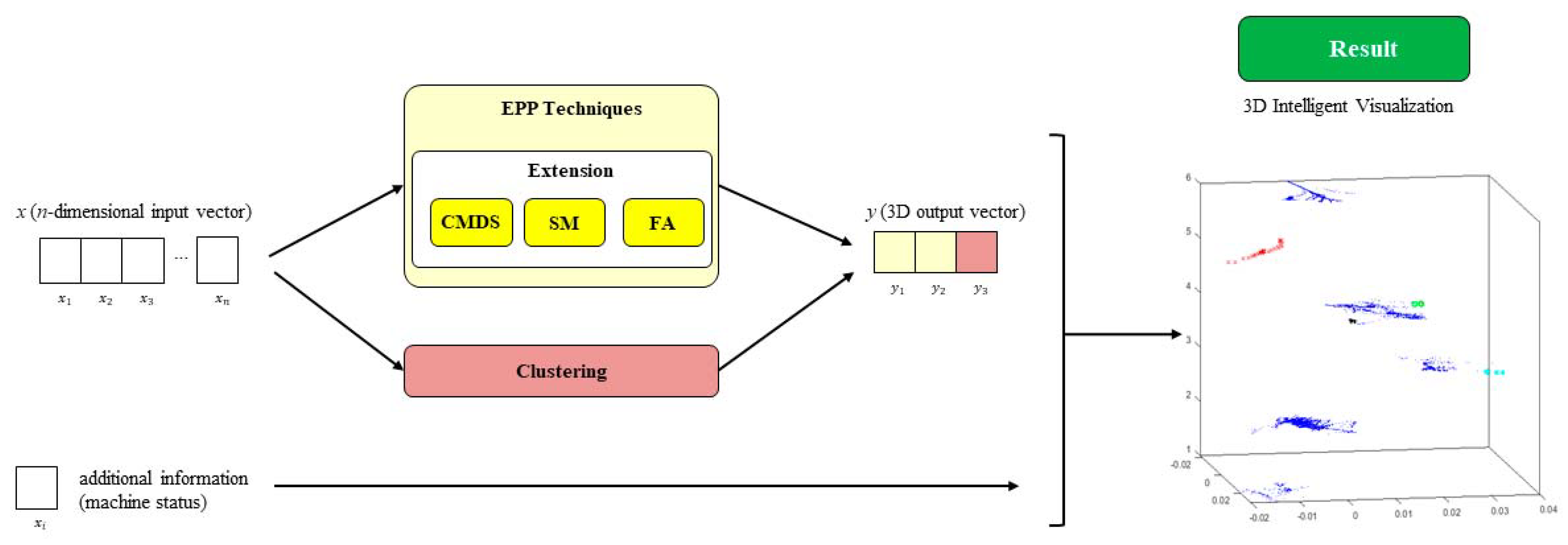
2. Hybrid Unsupervised Exploratory Plots

In order to extract knowledge from unlabelled datasets, many different methods could be applied. Among all of the ML methods, projection techniques are considered a viable approach for information seeking, as humans are able to recognize different features and to detect anomalies by inspecting graphs. Such patterns may become perceptible if variations are made to the spatial coordinates of the original datasets. However, an a priori choice regarding which parameters will reveal most patterns requires prior knowledge of unidentified patterns, and this is not an easy task. In order to do that, Exploratory Projection Pursuit (EPP) [8] is used for the purpose of data visualization. Contrasted with feature selection, EPP belongs to the feature extraction paradigm, as the resulting dimensions are combinations (could be linear or non-linear) of the original features in the dataset. Contrarily, clustering [9] is concerned with grouping together objects, that are similar to each other and dissimilar to objects belonging to other clusters. Therefore, patterns within the same cluster are more similar to each other than they are to a pattern belonging to a different cluster.
Recent work [7] has proposed the independent application of EPP techniques on the one hand, and clustering them on the other. The complete results of the two of them are then combined, together with the glyph metaphor, in a novel and different way, called the Hybrid Unsupervised Exploratory Plot (HUEP). HUEPs are a general-purpose approach, in which any EPP and clustering technique could be combined to generate 3D visualizations from high-dimensional data. In Figure 1, the process to generate a HUEP is shown. These depictions are informative and intuitive, not only for data scientists, but for all the company staff (not requiring previous knowledge regarding ML). Once a proper HUEP configuration has been selected by an expert, the other company staff will only need to analyze the obtained visualization. The HUEPs can be used by ‘non-expert’ professionals due to their simplicity, as no further decisions or parameter-tunings are required. The proposed HUEPs are hybrid as they combine both exploratory (dimensionality reduction) techniques with clustering ones. Besides, both types of technique are unsupervised as they apply this kind of learning (no target class or value is provided to be reproduced for new data instances).
In the original formulation of HUEPs [7], k-means [38] and Hierarchical Methods were applied as clustering techniques. Complementarily, PCA [39], MLHL [40] and CMLHL [41] were applied as EPP techniques. A wide variety of EPP techniques exists, but before this study, only the three previously-mentioned ones had been applied under the framework of HUEPs. Each EPP technique projects the data in a different way, thus for the same dataset the obtained visualizations could be very different. As happens for most of the data analysis problems, there is not a technique that always gets the best results for different datasets. Thus, depending on the analyzed data, one HUEP that uses a certain EPP method may be more suitable than another one. In keeping with this idea, we proposed in this study to extend HUEPs with other EPP techniques for a certain dataset. The main purpose is to validate that HUEPs can be extended with other EPP methods, and to prove that certain EPP methods could be more suitable than other ones when analyzing the present dataset.
The original HUEP formulation has been extended in the present study by incorporating and validating some additional EPP techniques, namely Classical Multidimensional Scaling (CMDS), Sammon Mapping (SM) and Factor Analysis (FA)—in yellow in Figure 1. They are described in the following subsections.

2.1. Classical Multidimensional Scaling

Multidimensional scaling (MDS) [42] is a set of methods that project high-dimensional data into a low-dimensional space using distances or dissimilarities. Classical MDS (CMDS) is a member MDS that shows the structure of distance-like data as a geometrical image [43]. Generally, MDS’s input is not a dataset, but the similarities of a set of items instead. CMDS uses a single distance matrix of Euclidian type as input.
CMDS is also known as Principal Coordinates Analysis (PCoA) [44], Torgerson Scaling or Torgerson–Gower scaling. It is often used to visualize data when only their distances or dissimilarities are available, but in this research, in order to extend and validate HUEPs with this family of methods, the original dataset has been reduced to a distance matrix. This matrix (pairwise distance between pairs of observations) creates a new configuration of points using the following metrics:
  • Euclidean;
  • Squared Euclidean;
  • Standardized Euclidean (seuclidean): each coordinate difference between observations is scaled by dividing by the corresponding element of the standard deviation;
  • Cityblock;
  • Minkowski;
  • Chebyshev: maximum coordinate difference;
  • Cosine: one minus the cosine of the included angle between points;
  • Correlation: one minus the sample correlation between points;
  • Hamming, which is the percentage of coordinates that differ;
  • Jaccard: one minus the Jaccard coefficient, which is the percentage of non-zero coordinates that differ;
  • Spearman: one minus the sample Spearman’s rank correlation between observations.

2.2. Sammon Mapping

Sammon Mapping (SM) [45,46] or Sammon Projection is a projection method for analyzing multivariate data. It can be seen as a type of MDS method, using a non-linear metric that is frequently used for EPP. SM maps a high-dimensional dataset to a lower dimensionality one, conserving the intrinsic structure of the data when the patterns are projected.
Unlike standard PCA and other EPP techniques, SM is a non-linear approach, as the result cannot be represented as a linear combination of the original variables. Nevertheless, SM minimizes the differences between corresponding pairwise point distances in the two spaces. PCA applies optimal mapping to the dataset, while SM tries to obtain a lower-dimensional dataset that keeps the original structure as much as possible. Because of that, the SM algorithm has a high computational load O(n2).
The source dataset is represented as N vectors in L-dimensional space, given by Xi, i = 1, ..., N. It is sought to map these into d-dimensional space (with d < L), to obtain vectors Yi, i = 1, ... N; dij is the pairwise distance between Yi and Yj, and dij* is the distance between Xi and Xj.
SM aims to minimize the following error function, which is often called Sammon’s stress or Sammon’s error:
E = 1 i < j d i j i < j n ( d i j d i j ) 2 d i j
As originally suggested [45], the minimization could be achieved by gradient searching techniques or by other methods, but these frequently involve iterative procedures. Convergent results are not always reached, and the number of iterations is decided experimentally [47].

2.3. Factor Analysis (FA)

Factor Analysis [48,49] is a data analysis technique that could be used for dimensionality reduction. It is used to reduce a large number of variables into a smaller set of factors, where factors refers to the lower number of unobserved or underlying variables. FA’s objective is to discover independent latent variables. It is frequently used with datasets with a large number of observed variables that could reveal a smaller number of underlying variables.
FA is differentiated from PCA as the former enforces a strict structure of a fixed number of common (latent) factors, while the latter defines p factors in decreasing order of importance. The main factor in FA is the one that, after rotation, provides the maximal interpretation, while the most significant factor in PCA is the one that maximizes the variance. Frequently, the main factor in FA is different from the direction of the first principal component. PCA extracts factors based on the total variance of the factors, but FA extracts factors based on the variance shared by the factors. PCA is used to find the smallest number of variables that explain the most variance, while FA is used to look for the latent underlying factors.

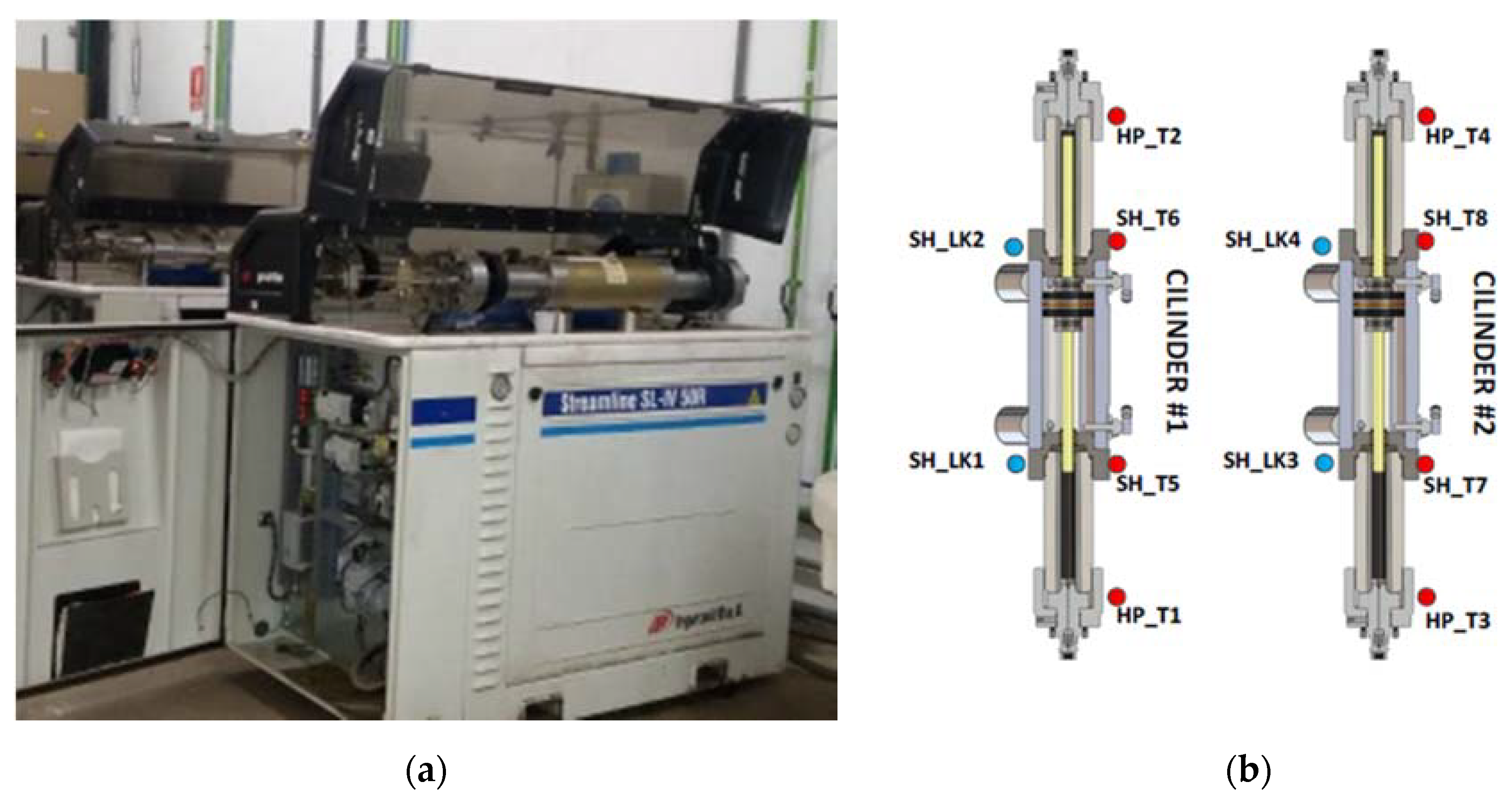
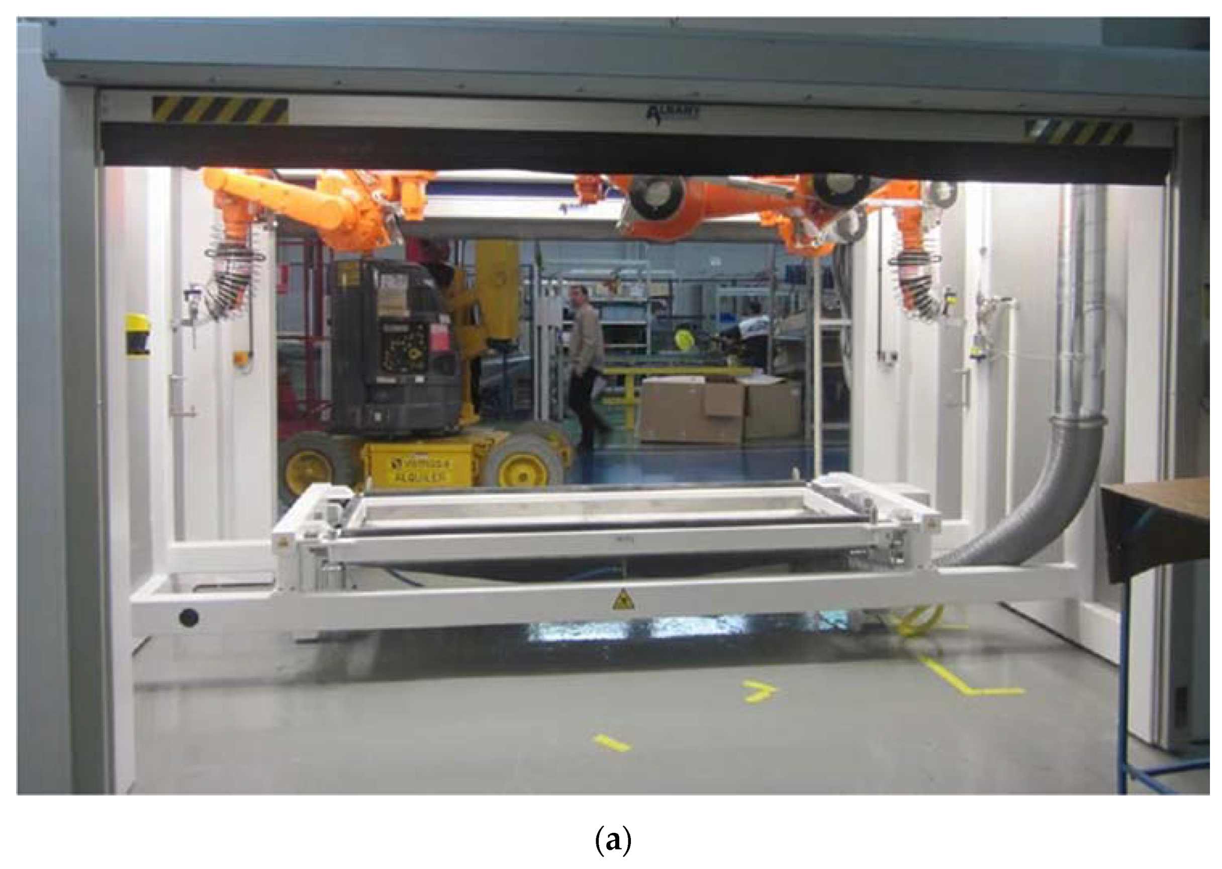
3. A Real Case Study: Waterjet Cutting

As previously stated, in order to validate the proposed HUEP extension, it has been applied to a case study involving a waterjet industrial tool. As a result, two datasets have been generated by collecting data from two different machines. HUEPs are generated in order to analyze these datasets, which comprise a great number of samples with a high number of features.
The machines under study are located in one factory from Grupo Antolin [10], a multinational company from the automotive industrial sector.
Waterjet cutting is used in various manufacturing industries (such as aerospace and automotive ones) for cutting, shaping, etc. [50]. This tool is used to cut several kinds of materials by means of an extremely high pressure jet of water, or a mixture of water and an abrasive substance. In the present work, the waterjet uses only water, and is applied during the fabrication of some parts manufactured in the factory. Two of its independent components have been selected for analysis due to their critical role:
  • Intensifier: the waterjet pumps or intensifiers [51], which supply water at extremely high pressure to waterjet machines;
  • Cyclone: the vacuum cyclone unit located in a waterjet machine, used for suctioning the waste generated towards a chute. It also holds the pieces during the cut.
To do this analysis, a time interval (February 2020) has been selected among all the available data as it includes samples of different anomalies/failures. As a consequence of the maintenance operations that are carried out, there are no anomalies most of the time, and it is not easy to find a period containing examples of some different anomalies.

3.1. Intensifier

The function of a water pump or intensifier (Figure 2) is to raise the water pressure to the level needed in the waterjet machines for an optimal operation. Explained in a very simple manner, the intensifier works like this: it begins when the low pressure water enters the intensifier (3–5 bar); after several filters, the water reaches a pump that raises the pressure to 10 bar, and then the water flows to the cylinders that will be compressed by a hydraulic group, which, using a plunger/piston system, will be able to reach an extremely high pressure (around 3000 bar) The intensifiers under study have two cylinders, as can be seen in Figure 2.
According to the experience of the workers in the plant, it is known that before a failure happens, an increase in temperature in different zones of the cylinder is observed. Another problem directly related with the increase of temperature is the water leaking, which is caused by the deterioration of the cylinder, and which can be visually observed. As this could lead to a critical failure, specific sensors have been installed in order to measure the temperature in the seal head (SH) and the hydraulic piston (HP) of the intensifier. Additionally, leak sensors have been installed in each cylinder. With the installation of these sensors, as shown in Figure 2, a diagnosis of the status of the machine could be performed in order to prevent failures.
The dataset analyzed in this research comprises 7414 samples (from February 2020) and 36 parameters (features), described in Table 1, which were gathered every 5 min (except for the increase of water leak).
As the intensifier has two cylinders and each cylinder has two SH and two HP, there are 36 total features: 4 temperature features per SH, 4 temperature features per HP, and 1 feature per SH for the leak problem. There is one temperature sensor per SH and HP, and one leak sensor per SH. As the features are recorded for a given time period, the maximum, minimum, average and standard deviation statistics are calculated during this period, and stored. In the case of the leak sensor, the increment when compared to the previous period is stored.
There are three main problems or failures that affect the intensifier:
  • Water leaks: the intensifier will stop working if there is a severe water leak. This is a critical failure with high associated costs, as it stops production;
  • High temperature in a cylinder: if high temperature lasts a long time, it could lead to a break in the header;
  • Detected SH malfunction; this means that it is necessary to repair the SH, or otherwise it will crash and stop the production. This malfunction/problem is perceived by the maintenance staff.

3.2. Cyclone

The following is the normal process when manufacturing a piece in the waterjet machine (Figure 3): the worker places a part inside the machine and gives the start order, and the cut operation is performed in a continuous way during the cycle. The water pressure generated by the intensifier reaches the level required by the robots in the waterjet for performing the complete cut of the piece. By means of a vacuum system, both the excess water and the cutting leftovers from the work are drained through a vacuum cyclone unit.
Cyclone failures are usually related to the vacuum system that the cyclone motor itself runs. This suction is responsible for securing the piece to be cut, in addition to absorbing the remaining water and cuttings leftover from the piece. The generated waste from the waterjet is suctioned towards a garbage chute. The most representative failures in this area are usually related to blockages in the suction circuit and air outlets, and vacuum malfunctioning. The data stored for detecting failures are related to the cyclone engine, and are obtained from the PLC. Additionally, vibration and temperature sensors have been installed in this motor in order to obtain more information about its status.
The dataset for this component comprises 623 samples (February 2020) and 24 parameters (features), described in Table 2, gathered for each manufacturing cycle.
Features are obtained from the machine PLC and from the device installed for detecting vibrations in the engine, as well as the temperature sensor. Data are stored in the cloud for each production cycle, the durations of which vary depending on the part that is being produced. The maximum, minimum, average and standard deviation statistics are calculated during the period and stored.
There are two main problems or failures that affect the cyclone:
  • The suction circuit is blocked: the waste absorbing system does not work properly. This is a critical failure as it stops production;
  • Vacuum malfunctioning: the vacuum does not work properly. It is an infrequent failure that does not stop production, but could lead to defective parts.

4. Results

The above-introduced HUEPs (see Section 2) have been applied to the real-world case study datasets described in the previous section. Plenty of different visualizations have been generated by combining all the EPPs (PCA, MLHL, CMLHL, CMDS, SM and FA) together with the clustering (k-means and agglomerative) techniques, tuned with different parameter values. However, for the sake of brevity, in this section only the main results are presented for comparison purposes. As no quantitative indicators have been developed yet to compare the level of goodness in a certain visualization, the obtained results are compared by taking into account one main criterion: whether the visualization lets users identify the anomalies, by depicting them as isolated from the other (“normal”) data samples. That is, “similar” data samples are visualized as groups separated from “dissimilar” data samples.
Different values were tested during experimentation for each one of the parameters associated with the applied models:
  • PCA: Number of output dimensions—2/3;
  • MLHL: Number of output dimensions—2/3; number of iterations—1000/2000/3000; learning rate—0.01/0.005/0.001; p—0.1/0.5;
  • CMLHL: Number of output dimensions—2/3; number of iterations—1000/2000/3000; learning rate—0.01/0.005/0.001; p—0.1/0.5; τ—0.05;
  • CMDS: Number of output dimensions—2/3; distance metrics—Euclidean/Squared Euclidean/Standardized Euclidean/Cityblock/Minkowski/Chebyshev/Cosine/Correlation/Jaccard/Spearman;
  • SM: Number of output dimensions—2/3; number of iterations—100/200/500;
  • FA: Number of output dimensions—2/3; 200 iterations maximum;
  • k-means: Distances—Squared Euclidean/Cityblock/Cosine/Correlation; k—3/4/6/8;
  • Agglomerative clustering: Distances—Euclidean/Chebyshev/Minkowski/Correlation/Seuclidean/Squared Euclidean/Cityblock/Mahalanobis/Cosine/Spearman/Hamming/Jaccard; linkages—average/centroid/complete/median/single/ward/weighted; a cutoff value adjusted to obtain the same number of clusters as in the case of k-means (3/4/6/8).

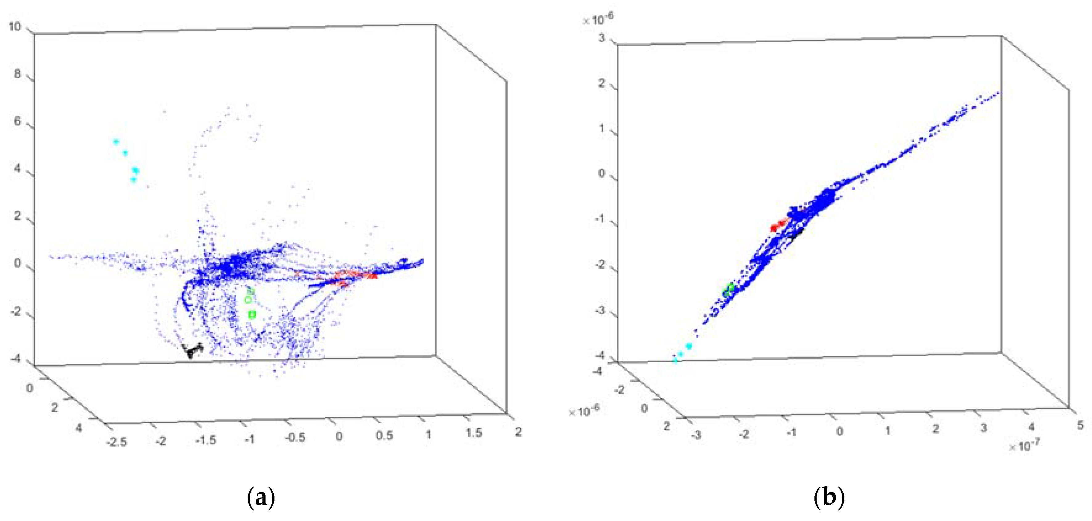
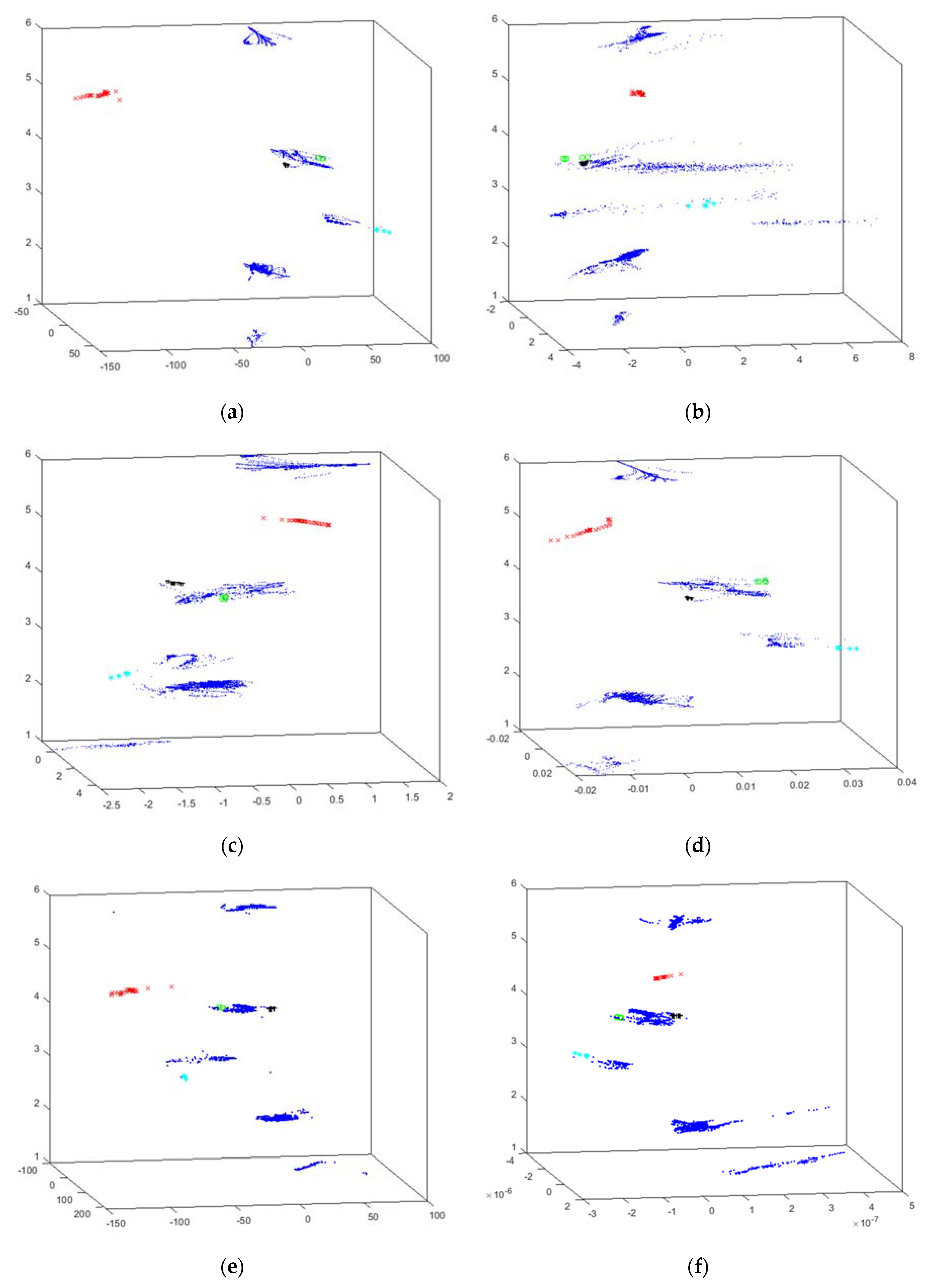
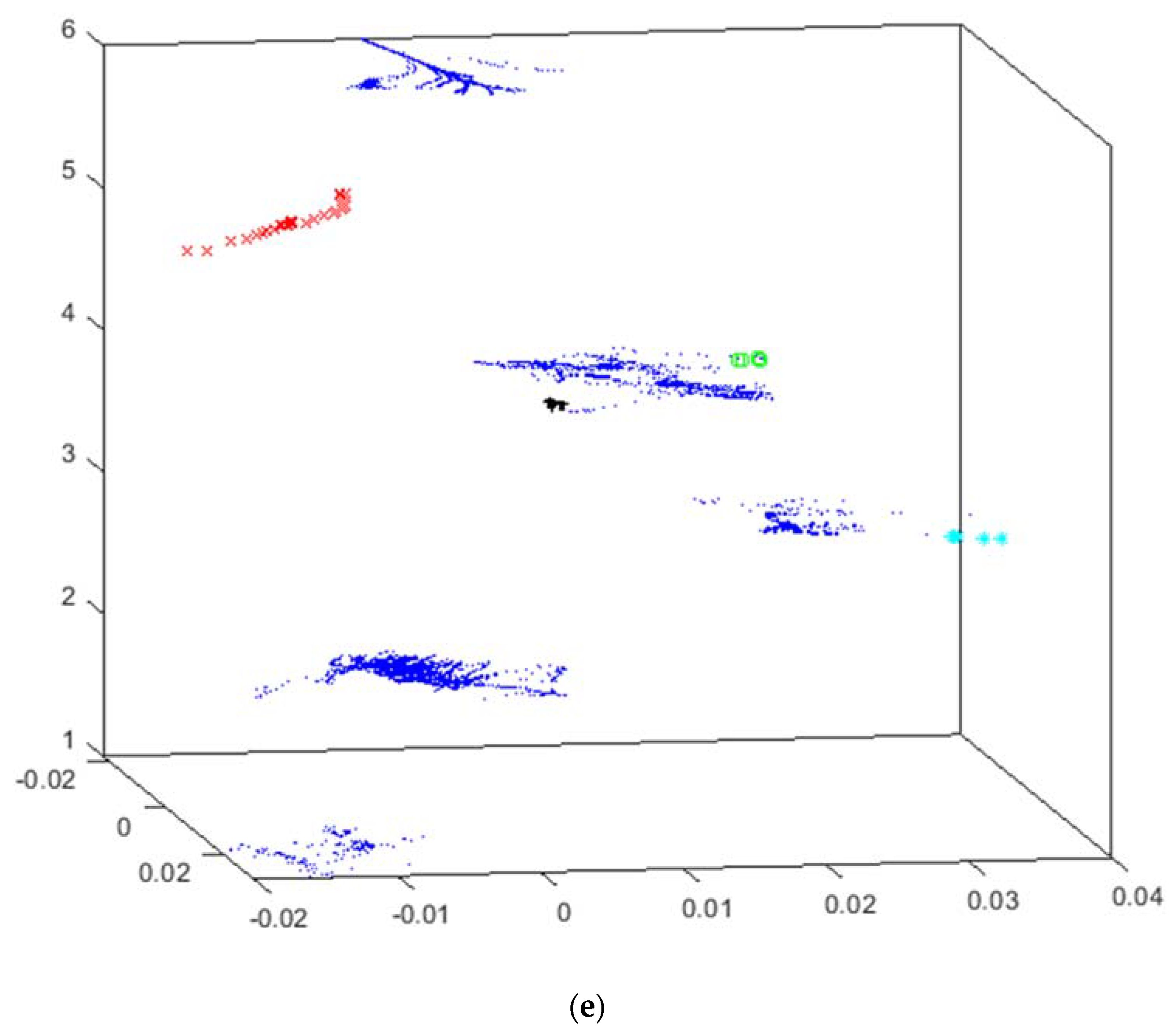
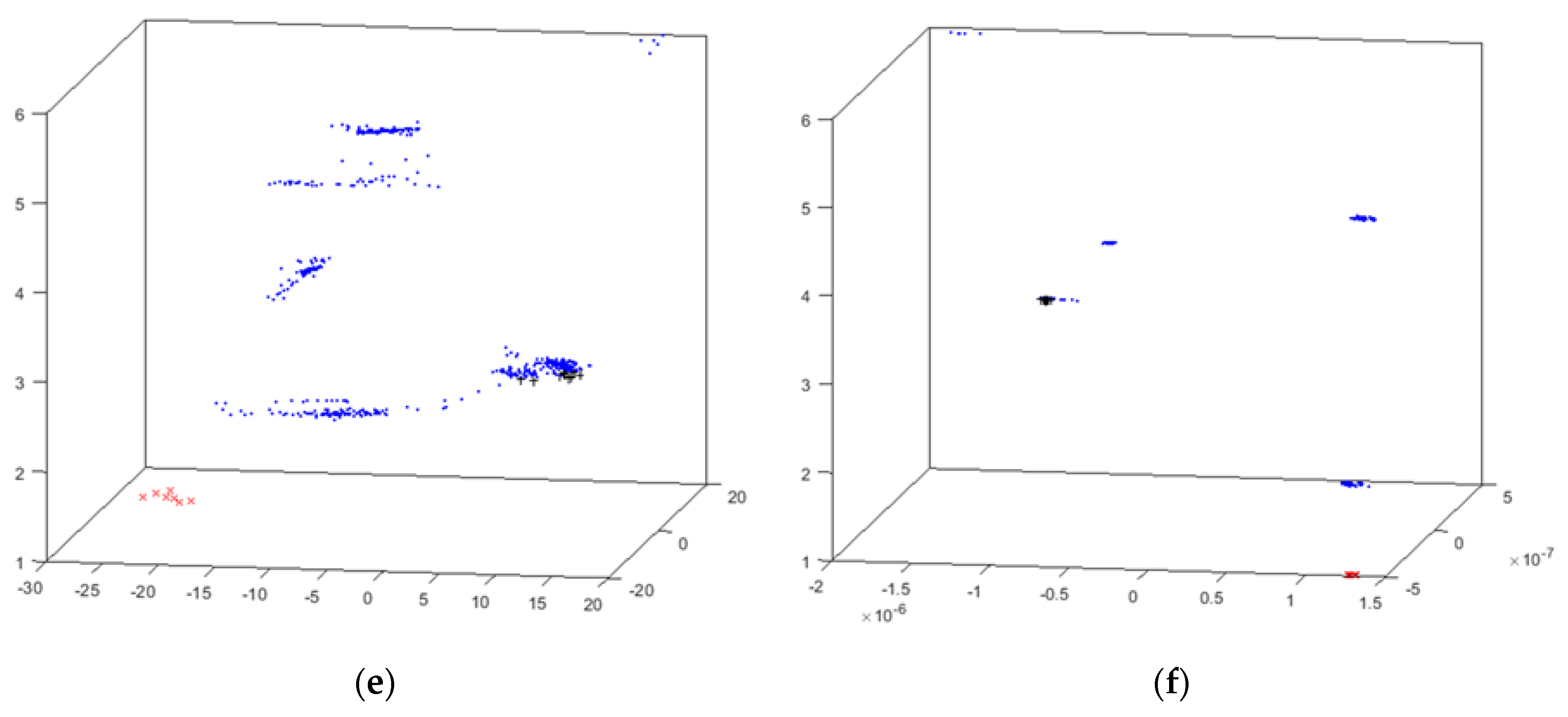
4.1. Intensifiers Results

Results shown in this section include visualizations of all the data samples in the intensifier dataset. Each one of them is depicted by adding the following extra information (related to the machine status) through the glyph metaphor:
  • x (red x): water leak;
  • + (black +): high temperature in cylinder #1;
  • * (cyan *): high temperature in cylinder #2;
  • o (green o): detected SH malfunctioning;
  • · (blue point): no problem reported (i.e., intensifier properly working).
Initially, the two best EPP 3D projections (CMLHL and FA) are shown in Figure 4. These simple visualizations (the right-straight outputs of the EPP methods) are shown for comparison purposes, in order to contrast them with the obtained HUEP visualizations (see below).
It can be observed that CMLHL (Figure 4a) does not show the principal failure (red x) separated from the other data instances, and that FA (Figure 4b) does not show any data grouping and all the samples are mixed. However, in the FA projection, some of the anomalies are somehow grouped, but not isolated from the other ones.
The best results generated by the HUEPs are presented in Figure 5. Each figure shows the result obtained by the corresponding HUEP, as stated in the label; i.e., the combinations of the EPP method—for example, (a) shows PCA combined with the hierarchical clustering method, tuned according to the given parameter values [for example, 6 clusters (k parameter), using Cityblock as distance metric and Complete as linkage method]. In all the HUEP figures, the cluster number assigned to each data instance is shown in the vertical (z) axis. For example, in Figure 5, all the results are grouped in 6 clusters, so values 1 to 6 are shown on the z axis of all the HUEPs.
Regarding the results obtained with the extended HUEPs, it can be said that adding the clustering information to the EPP projection leads to a significant improvement in the visualization. This can be clearly seen in the case of the main failure (red x), as all these data samples are assigned to the same cluster (number 5), and thus isolated from the other ones.
When comparing the applied EPP methods, CMDS (Figure 5d and Figure 6e) outperforms the other ones, as in this projection it can be observed that all the data samples associated to failures or problems are separated from the “normal” points (in blue). All in all, it can be concluded that the three novel EPP techniques (CMDS, SM and FA), when combined with a clustering technique in a HUEP, offer more information than the EPP projection on its own. If the FA projection (Figure 4b) is compared to the HUEP obtained from FA and hierarchical clustering [k = 6, Cityblock, and complete (Figure 5f)], it can be said that the visualization is much more informative.
As CMDS is the EPP method that generates the best HUEP for this dataset, additional results obtained with this method are shown in Figure 6. The main purpose of this figure is to compare the visualizations generated when varying clustering parameters.
In Figure 6, the same CMDS–Cityblock projection is combined with k-means and hierarchical clustering outputs. As can be seen, the hierarchical clustering can separate into independent groups the critical-failure data (red x). Opposingly, the k-means does not separate these critical samples into a unique group, splitting these data into two different groups. When increasing the number of clusters (k), data are more separated, and hence visualizations are more informative. It can be said that hierarchical clustering is the method that generates better visualizations when combined with CMDS in a HUEP for the intensifier dataset. More precisely, Figure 6e presents the best of the HUEP visualizations generated for this dataset.

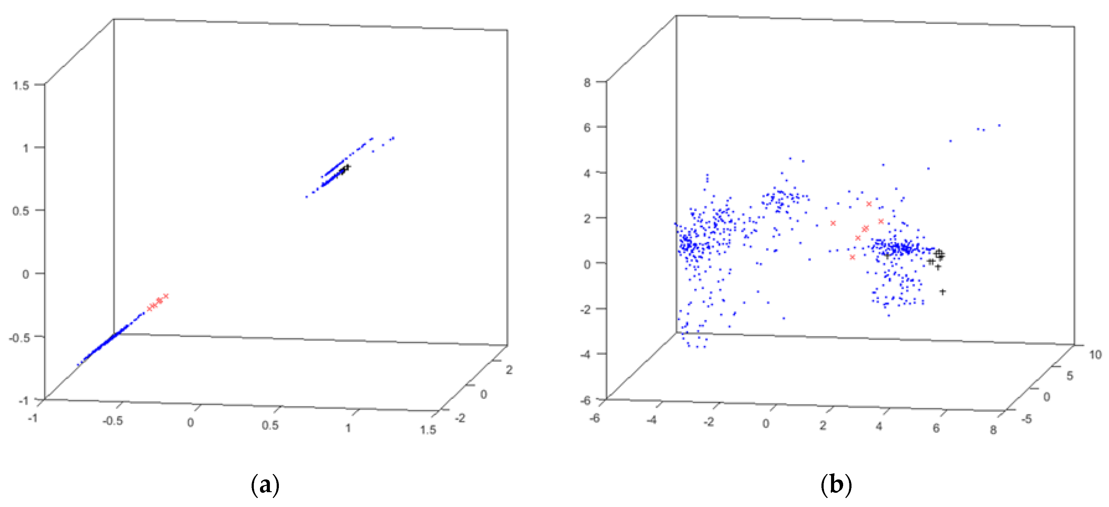
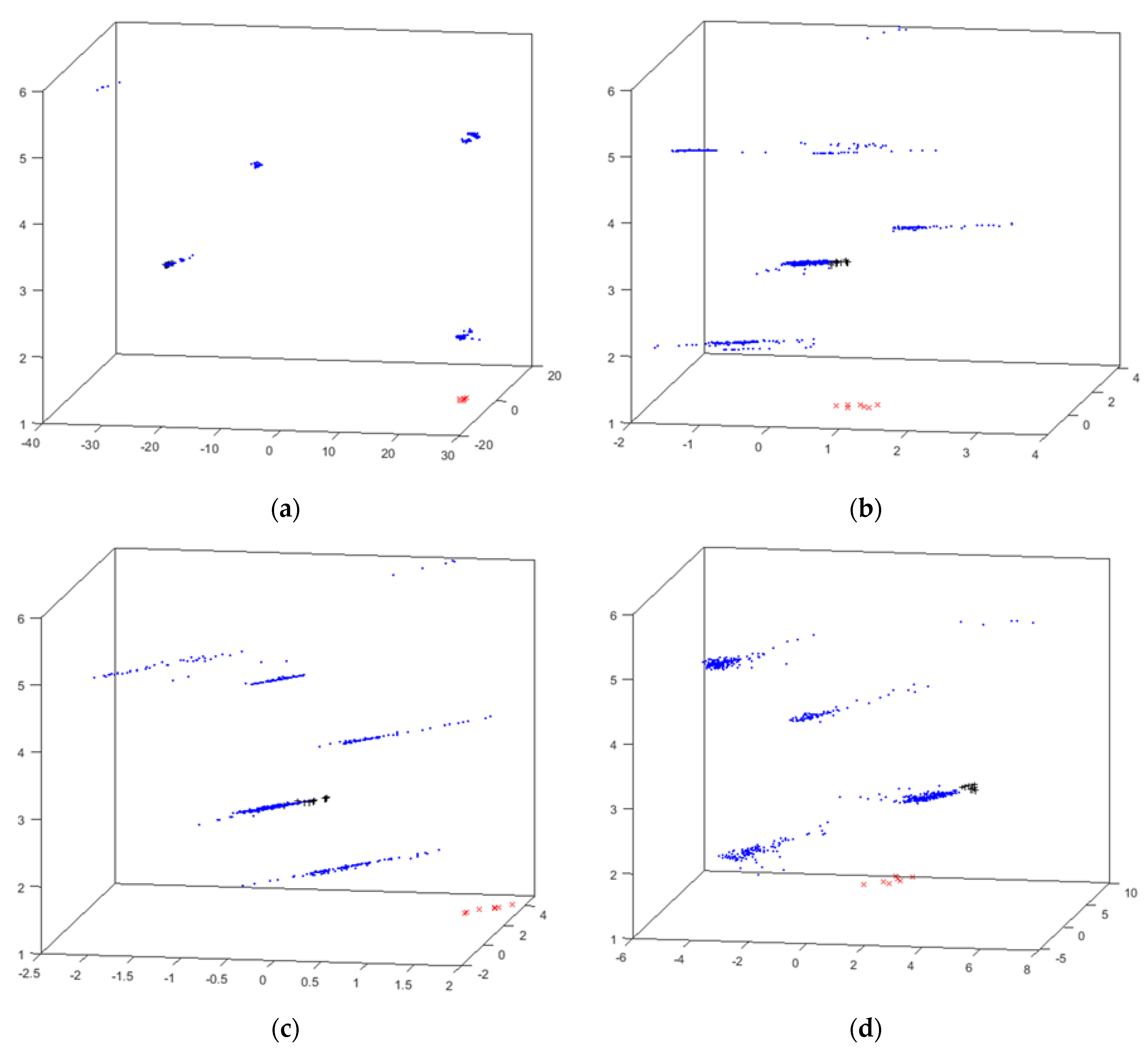
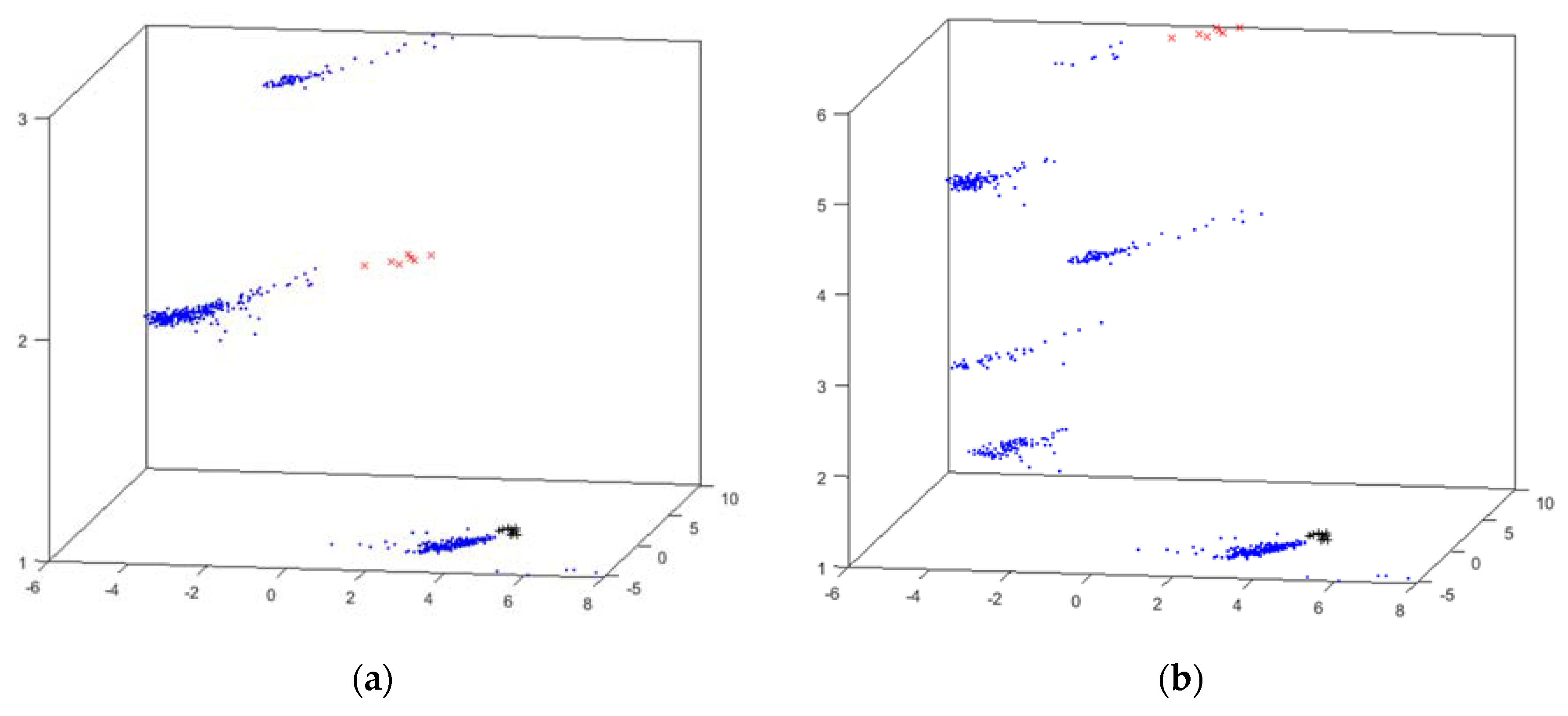
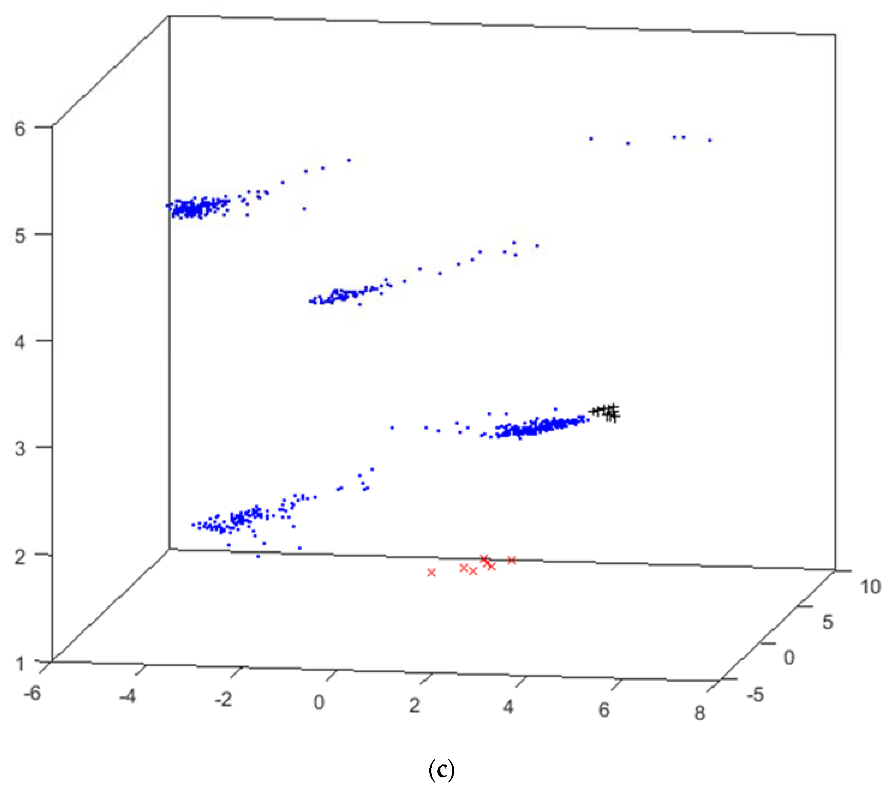
4.2. Cyclone Results

Results shown in this section include visualizations of all the data samples in the Cyclone dataset. Each one of them is depicted by adding the following extra information (related to the machine status) through the glyph metaphor:
  • x (red x): suction circuit is blocked;
  • + (black +): vacuum malfunctioning;
  • · (blue point): no problem reported (i.e., cyclone properly working).
As for the previous dataset, the best EPP visualizations are shown in Figure 7. In this case, the selected ones are the CMLHL (Figure 7a) and CMDS (Figure 7b) projections.
It can be observed that none of the EPP techniques generate a visualization that clearly separates the data samples associated to anomalies. These projections are significantly enhanced when combined with the clustering results in the HUEPs, as shown in Figure 8.
As has been shown for the previous dataset, it is worth mentioning that CMDS generates the best HUEPs for the cyclone dataset. The best result is obtained with CMDS with Seuclidean + hierarchical clustering (k = 6, Cityblock, and weighted), shown in Figure 8d and Figure 9c. In these visualizations, the critical failure (suction circuit is blocked) samples (red x) are isolated in a unique group, as are those samples associated to the other anomaly (black +), which are also depicted in a separated group. The HUEPs generated for this dataset can clearly visualize the critical failure in a separate group. This is done thanks to the combination with clustering results; the samples associated to the main failure are grouped in the same cluster, clearly visualizing them in a separate group. Although the samples from the other anomaly (vacuum malfunctioning) are clustered with many “normal” samples, the CMDS projection visualizes them in a separate way.
Once again, CMDS is the EPP method generating the best HUEP, and additional results obtained with this method are shown in Figure 9. The main purpose of this figure is to compare the visualizations generated when clustering parameters are varied.
Figure 9 shows the results obtained by combining CMDS–Seuclidean with k-means and hierarchical clustering. The hierarchical clustering method can separate into cluster #1 the critical-failure samples (red x), but k-means groups these data together with “normal” samples. It can thus be said that, as in the case of the previous dataset, hierarchical clustering leads to better visualization results for the cyclone dataset.
In general terms, the HUEPs generated by agglomerative (hierarchical) clustering are more informative than those generated by k-means for the two datasets under analysis. This is consistent with general heuristics [52], as agglomerative clustering is more appropriate if groups are expected to be different sizes. Opposingly, k-means is the best option when the expected groups have approximately similar sizes. In the two analyzed datasets, there are many more data samples associated with the “normal” functioning of the components than those associated with failures. Consequently, the HUEPs’ would have better visualizations by using agglomerative clustering rather than k-means. The validations carried out with both datasets have shown that HUEPs generated by CMDS are the most useful ones, as they provide visualizations that separate failures from “normal” samples in the clearest way.

5. Conclusions and Future Work

This study has shown that HUEPs are a technique that supports the monitoring of sensors and machines in order to anticipate failures. Firstly, it can be used to easily see that the data that has been gathered have a structure, and that they could be representative and informative. Then, HUEPs can show separate groups, differentiating failures from normal functioning. The proposed HUEP extension supports decision-making as it depicts data in a visual way that assists with this task. This has been tested and validated in a complex industrial scenario, with associated datasets comprising a great number of samples and a high number of features. As a result, PdM can be carried out in a manner complementary to other tools, anticipating deviations in operating conditions.
It has been proven that the proposed extension of HUEPs outperforms the original formulation in visualizing the datasets from the present case study. It is worth mentioning that HUEPs generated by CMDS are more useful than the other ones, as the different anomalies are grouped and visualized in a clearer way. Additionally, CMDS is an interesting EPP technique because it can be applied with several distance metrics that adjust to the dataset under study. On the other hand, for the analyzed datasets (where the “normal” samples are more numerous than the failure ones), agglomerative clustering groups data in a more consistent way than k-means.
It has been proven that, depending on the dataset, it could be better to use a combination of methods, to generate one HUEP or another. That is, the best visualizations for the intensifier are not generated with the same parameter combination as that used for the cyclone dataset. Hence, it is important to carry out an exhaustive experimentation with every different combination, in order to identify the best visualization. Once this is performed, any person familiar with the manufacturing process (such as skilled operators and maintenance staff, among others) would be qualified to analyze the visualizations obtained, and take decisions based on them.
As a future line of work, authors propose the combination of HUEPs with the outputs of supervised models, in order to implement a holistic tool. Furthermore, a tool is proposed that generates specific visualizations for machine operators and maintenance staff. This would help them in supervising the manufacturing and in completing the machine’s maintenance. Additionally, HUEPs are being applied to some other components/machines, in order to validate their ability for operation monitoring and failure detection. The use of HUEPs for quality purposes will also be explored, in order to improve the detection of quality defects.

Author Contributions

Conceptualization, Á.H., E.C. and J.S.; methodology, Á.H.; software, R.R.; formal analysis, R.R. and Á.H.; data curation R.R.; writing—original draft preparation, R.R. and Á.H.; writing—review and editing, R.R., Á.H., E.C. and J.S.; supervision, Á.H., E.C. and J.S. All authors have read and agreed to the published version of the manuscript.

Funding

This research received no external funding.

Acknowledgments

The authors would like to thank the vehicle interiors manufacturer, Grupo Antolin, for its collaboration in this research.

Conflicts of Interest

The authors declare no conflict of interest.

Abbreviations

The following abbreviations are used in this manuscript, in alphabetic order:
ANNArtificial Neural Networks
CMDSClassical Multidimensional Scaling
CMLHLCooperative Maximum-Likelihood Hebbian Learning
EPPExploratory Projection Pursuit
FAFactor Analysis
FDFailure Detection
HPHydraulic Piston
HUEPHybrid Unsupervised Exploratory Plot
IoTInternet of Things
KNNk-Nearest Neighbour
MDSMultidimensional scaling
MLMachine Learning
MLHLMaximum-Likelihood Hebbian Learning
PCAPrincipal Component Analysis
PdMPredictive Maintenance
SHSeal Head
SMSammon Mapping

References

  1. Zhou, K.; Liu, T.; Zhou, L. Industry 4.0: Towards Future Industrial Opportunities and Challenges. In Proceedings of the 2015 12th International Conference on Fuzzy Systems and Knowledge Discovery (FSKD), Zhangjiajie, China, 15–17 August 2015; pp. 2147–2152. [Google Scholar] [CrossRef]
  2. Khan, M.; Xiaotong, W.; Xiaolong, X.; Wanchun, D. Big Data Challenges and Opportunities in the Hype of Industry 4.0. In Proceedings of the 2017 IEEE International Conference on Communications (ICC), Paris, France, 21–25 May 2017. [Google Scholar] [CrossRef]
  3. Del Campo, G.; Calatrava, S.; Canada, G.; Olloqui, J.; Martinez, R.; Santamaria, A. IoT Solution for Energy Optimization in Industry 4.0: Issues of a Real-Life Implementation. In Proceedings of the 2018 Global Internet of Things Summit (GIoTS), Bilbao, Spain, 4–7 June 2018. [Google Scholar] [CrossRef]
  4. Vathoopan, M.; Johny, M.; Zoitl, A.; Knoll, A. Modular Fault Ascription and Corrective Maintenance Using a Digital Twin. In Proceedings of the 16th IFAC Symposium on Information Control Problems in Manufacturing INCOM 2018, Bergamo, Italy, 11–13 June 2018; pp. 1041–1046. [Google Scholar] [CrossRef]
  5. Shafiq, S.I.; Szczerbicki, E.; Sanin, C. Manufacturing Data Analysis in Internet of Things/Internet of Data (IoT/IoD) Scenario. Cybern. Syst. 2018, 49, 280–295. [Google Scholar] [CrossRef]
  6. Qu, Y.J.; Ming, X.G.; Liu, Z.W.; Zhang, X.Y.; Hou, Z.T. Smart Manufacturing Systems: State of the Art and Future Trends. Int. J. Adv. Manuf. Technol. 2019, 103, 3751–3768. [Google Scholar] [CrossRef]
  7. Herrero, Á.; Jiménez, A.; Bayraktar, S. Hybrid Unsupervised Exploratory Plots: A Case Study of Analysing Foreign Direct Investment. Complexity 2019, 2019. [Google Scholar] [CrossRef]
  8. Friedman, J.H. Exploratory Projection Pursuit. J. Am. Stat. Assoc. 1987, 82, 249–266. [Google Scholar] [CrossRef]
  9. Jain, A.K.; Murty, M.N.; Flynn, P.J. Data Clustering: A Review. ACM Comput. Surv. 1999, 31, 264–323. [Google Scholar] [CrossRef]
  10. Grupo Antolin. Available online: https://www.grupoantolin.com/ (accessed on 14 May 2020).
  11. Para, J.; Del Ser, J.; Nebro, A.J.; Zurutuza, U.; Herrera, F. Analyze, Sense, Preprocess, Predict, Implement, and Deploy (ASPPID): An Incremental Methodology Based on Data Analytics for Cost-Efficiently Monitoring the Industry 4.0. Eng. Appl. Artif. Intell. 2019, 82, 30–43. [Google Scholar] [CrossRef]
  12. Skiena, S.S. Visualizing Data. In The Data Science Design Manual; Texts in Computer Science; Springer: Cham, Switzerland, 2017; pp. 155–200. [Google Scholar] [CrossRef]
  13. Posada, J.; Toro, C.; Barandiaran, I.; Oyarzun, D.; Stricker, D.; De Amicis, R.; Pinto, E.B.; Eisert, P.; Döllner, J.; Vallarino, I. Visual Computing as a Key Enabling Technology for Industrie 4.0 and Industrial Internet. IEEE Comput. Graph. Appl. 2015, 35, 26–40. [Google Scholar] [CrossRef]
  14. Segura, Á.; Diez, H.V.; Barandiaran, I.; Arbelaiz, A.; Álvarez, H.; Simões, B.; Posada, J.; García-Alonso, A.; Ugarte, R. Visual Computing Technologies to Support the Operator 4.0. Comput. Ind. Eng. 2020, 139, 105550. [Google Scholar] [CrossRef]
  15. Posada, J.; Zorrilla, M.; Dominguez, A.; Simões, B.; Eisert, P.; Stricker, D.; Rambach, J.; Dollner, J.; Guevara, M. Graphics and Media Technologies for Operators in Industry 4.0. IEEE Comput. Graph. Appl. 2018, 38, 119–132. [Google Scholar] [CrossRef]
  16. Jimenez-Cortadi, A.; Irigoien, I.; Boto, F.; Sierra, B.; Rodriguez, G. Predictive Maintenance on the Machining Process and Machine Tool. Appl. Sci. 2020, 10, 224. [Google Scholar] [CrossRef] [Green Version]
  17. Uhlmann, E.; Pontes, R.P.; Geisert, C.; Hohwieler, E. Cluster Identification of Sensor Data for Predictive Maintenance in a Selective Laser Melting Machine Tool. In Proceedings of the 4th International Conference on System-Integrated Intelligence: Intelligent, Flexible and Connected Systems in Products and Production, Hannover, Germany, 19–20 June 2018; pp. 60–65. [Google Scholar] [CrossRef]
  18. Diez-Olivan, A.; Pagán, J.A.; Sanz, R.; Sierra, B. Data-Driven Prognostics Using a Combination of Constrained K-Means Clustering, Fuzzy Modeling and LOF-Based Score. Neurocomputing 2017, 241, 97–107. [Google Scholar] [CrossRef] [Green Version]
  19. Yoo, Y.; Park, S.H.; Baek, J.-G. A Clustering-Based Equipment Condition Model of Chemical Vapor Deposition Process. Int. J. Precis. Eng. Manuf. 2019, 1677–1689. [Google Scholar] [CrossRef]
  20. Jia, F.; Lei, Y.; Guo, L.; Lin, J.; Xing, S. A Neural Network Constructed by Deep Learning Technique and Its Application to Intelligent Fault Diagnosis of Machines. Neurocomputing 2018, 272, 619–628. [Google Scholar] [CrossRef]
  21. Lei, Y.; Jia, F.; Lin, J.; Xing, S.; Ding, S.X. An Intelligent Fault Diagnosis Method Using Unsupervised Feature Learning Towards Mechanical Big Data. IEEE Trans. Ind. Electron. 2016, 63, 3137–3147. [Google Scholar] [CrossRef]
  22. Delgado-Prieto, M.; Cirrincione, G.; Espinosa, A.G.; Ortega, J.A.; Henao, H. Bearing Fault Detection by a Novel Condition-Monitoring Scheme Based on Statistical-Time Features and Neural Networks. IEEE Trans. Ind. Electron. 2013, 60, 3398–3407. [Google Scholar] [CrossRef]
  23. Pacheco, F.; De Oliveira, J.V.; Sánchez, R.-V.; Cerrada, M.; Cabrera, D.; Li, C.; Zurita, G.; Artés, M. A Statistical Comparison of Neuroclassifiers and Feature Selection Methods for Gearbox Fault Diagnosis under Realistic Conditions. Neurocomputing 2016, 194, 192–206. [Google Scholar] [CrossRef]
  24. Jia, F.; Lei, Y.; Lin, J.; Zhou, X.; Lu, N. Deep Neural Networks: A Promising Tool for Fault Characteristic Mining and Intelligent Diagnosis of Rotating Machinery with Massive Data. Mech. Syst. Signal Process. 2016, 72–73, 303–315. [Google Scholar] [CrossRef]
  25. Yang, Y.-H.; Pan, Y.-K.; Zhang, L.-P.; Liu, X.-Z. Incipient Fault Detection Method Based on Stream Data Projection Transformation Analysis. IEEE Access 2019, 7, 93062–93075. [Google Scholar] [CrossRef]
  26. Li, X.; Zhang, W.; Ding, Q. A Robust Intelligent Fault Diagnosis Method for Rolling Element Bearings Based on Deep Distance Metric Learning. Neurocomputing 2018, 310, 77–95. [Google Scholar] [CrossRef]
  27. Lei, Y.; He, Z.; Zi, Y.; Chen, X. New Clustering Algorithm-Based Fault Diagnosis Using Compensation Distance Evaluation Technique. Mech. Syst. Signal Process. 2008, 22, 419–435. [Google Scholar] [CrossRef]
  28. Liu, H.; Zhou, J.; Xu, Y.; Zheng, Y.; Peng, X.; Jiang, W. Unsupervised Fault Diagnosis of Rolling Bearings Using a Deep Neural Network Based on Generative Adversarial Networks. Neurocomputing 2018, 315, 412–424. [Google Scholar] [CrossRef]
  29. Jianbo, Y. Local and Nonlocal Preserving Projection for Bearing Defect Classification and Performance Assessment. IEEE Trans. Ind. Electron. 2012, 59, 2363–2376. [Google Scholar] [CrossRef]
  30. Li, W.; Zhang, S.; Rakheja, S. Feature Denoising and Nearest–Farthest Distance Preserving Projection for Machine Fault Diagnosis. IEEE Trans. Ind. Inform. 2016, 12, 393–404. [Google Scholar] [CrossRef]
  31. Chen, X.-L.; Wang, P.-H.; Hao, Y.-S.; Zhao, M. Evidential KNN-Based Condition Monitoring and Early Warning Method with Applications in Power Plant. Neurocomputing 2018, 315, 18–32. [Google Scholar] [CrossRef]
  32. Wang, D. K-Nearest Neighbors Based Methods for Identification of Different Gear Crack Levels under Different Motor Speeds and Loads: Revisited. Mech. Syst. Signal Process. 2016, 70–71, 201–208. [Google Scholar] [CrossRef]
  33. Luwei, K.C.; Yunusa-Kaltungo, A.; Sha’Aban, Y. Integrated Fault Detection Framework for Classifying Rotating Machine Faults Using Frequency Domain Data Fusion and Artificial Neural Networks. Machines 2018, 6, 59. [Google Scholar] [CrossRef] [Green Version]
  34. You, D.; Gao, X.; Katayama, S. WPD-PCA-Based Laser Welding Process Monitoring and Defects Diagnosis by Using FNN and SVM. IEEE Trans. Ind. Electron. 2015, 62, 628–636. [Google Scholar] [CrossRef]
  35. Zhao, C.; Gao, F. Fault-Relevant Principal Component Analysis (FPCA) Method for Multivariate Statistical Modeling and Process Monitoring. Chemom. Intell. Lab. Syst. 2014, 133, 1–16. [Google Scholar] [CrossRef]
  36. Deng, X.; Tian, X.; Chen, S.; Harris, C.J. Fault Discriminant Enhanced Kernel Principal Component Analysis Incorporating Prior Fault Information for Monitoring Nonlinear Processes. Chemom. Intell. Lab. Syst. 2017, 162, 21–34. [Google Scholar] [CrossRef] [Green Version]
  37. Yang, Y.-H.; Chen, X.; Zhang, Y.; Liu, X. A Novel Decentralized Weighted ReliefF-PCA Method for Fault Detection. IEEE Access 2019, 7, 140478–140487. [Google Scholar] [CrossRef]
  38. MacQueen, J.B. Some Methods for Classification and Analysis of Multivariate Observations; Western Management Science International University of California: Los Angeles, CA, USA, 1966. [Google Scholar]
  39. Jolliffe, I.T. Principal Component Analysis; (Springer Series in Statistics); Springer-Verlag: New York, NY, USA, 2002. [Google Scholar] [CrossRef]
  40. Corchado, E.; Macdonald, D.; Fyfe, C. Maximum and Minimum Likelihood Hebbian Learning for Exploratory Projection Pursuit. Data Min. Knowl. Discov. 2004, 8, 203–225. [Google Scholar] [CrossRef] [Green Version]
  41. Corchado, E.; Fyfe, C. Connectionist Techniques for the Identification and Suppression of Interfering Underlying Factors. Int. J. Pattern Recognit. Artif. Intell. 2003, 17, 1447–1466. [Google Scholar] [CrossRef]
  42. Torgerson, W.S. Multidimensional Scaling: I. Theory and Method. Psychometrika 1952, 17, 401–419. [Google Scholar] [CrossRef]
  43. Wang, J. Classical Multidimensional Scaling. Geom. Struct. High-Dimens. Data Dimens. Reduct. 2012, 115–129. [Google Scholar] [CrossRef]
  44. Gower, J.C. Principal Coordinates Analysis. In Wiley StatsRef: Statistics Reference Online; American Cancer Society: Atlanta, GA, USA, 2015; pp. 1–7. [Google Scholar] [CrossRef]
  45. Sammon, J.W. A Nonlinear Mapping for Data Structure Analysis. IEEE Trans. Comput. 1969, C–18, 401–409. [Google Scholar] [CrossRef]
  46. Henderson, P. Sammon mapping. Pattern Recognit. Lett. 1997, 18, 1307–1316. [Google Scholar]
  47. Lerner, B.; Guterman, H.; Aladjem, M.; Dinstein, I. On the Initialisation of Sammon’s Nonlinear Mapping. Pattern Anal. Appl. 2000, 3, 61–68. [Google Scholar] [CrossRef] [Green Version]
  48. Härdle, W.K.; Simar, L. Factor Analysis. Appl. Multivar. Stat. Anal. 2015, 359–384. [Google Scholar] [CrossRef]
  49. Cleff, T. Factor Analysis. Appl. Stat. Multivar. Data Anal. Bus. Econ. 2019, 433–446. [Google Scholar] [CrossRef]
  50. Kong, C. Water-Jet Cutting. CIRP Encycl. Prod. Eng. 2019, 1803–1807. [Google Scholar] [CrossRef]
  51. KMT Streamline SL-V Pumps Catalog.Pdf. Available online: https://www.kmtwaterjet.com/KMT%20Streamline%20SL-V%20Pumps%20Catalog.pdf (accessed on 14 May 2020).
  52. Cleophas, T.J.; Zwinderman, A.H. Density-Based Clustering to Identify Outlier Groups in Otherwise Homogeneous Data (50 Patients). Mach. Learn. Med. Cookb. 2014, 9–11. [Google Scholar] [CrossRef]
Figure 1. Process to obtain a HUEP.
Applsci 10 04355 g001
Figure 2. Example of intensifier and sketch of sensors (blue and red circles). (a) Picture of the intensifier. (b) Sensors placement sketch.
Applsci 10 04355 g002
Figure 3. Example of a waterjet machine with the cyclone and sketch of sensors (red and green circles). (a) Waterjet machine. (b) Sensors placement sketch.
Applsci 10 04355 g003aApplsci 10 04355 g003b
Figure 4. 3D visualizations generated by EPP methods for the intensifier dataset. (a) CMLH 3D visualization. (b) FA 3D visualization.
Applsci 10 04355 g004
Figure 5. HUEP visualizations of the intensifier dataset. EPP+hierarchical clustering. (a) HUEP: PCA+hierarchical clustering (k = 6, Cityblock, and complete). (b) HUEP: MLHL+hierarchical clustering (k = 6, Cityblock, and complete). (c) HUEP: CMLHL+hierarchical clustering (k = 6, Cityblock, and complete). (d) HUEP: CMDS–cityblock+hierarchical clustering (k = 6, Cityblock, and complete). (e) HUEP: SM+hierarchical clustering (k = 6, Cityblock, and complete). (f) HUEP: FA+hierarchical clustering (k = 6, Cityblock, and complete).
Applsci 10 04355 g005
Figure 6. HUEP visualizations generated by CMDS–Cityblock and different clustering parameters of the intensifier dataset. (a) HUEP: CMDS–Cityblock+k-means (k = 3 and Cityblock). (b) HUEP: CMDS–Cityblock+k-means (k = 6 and Cityblock). (c) HUEP: CMDS–Cityblock+hierarchical clustering (k = 4, Minkowski, and weighted). (d) HUEP: CMDS–Cityblock+hierarchical clustering (k = 6, Chebyshev, and complete). (e) HUEP: CMDS–Cityblock+hierarchical clustering (k = 6, Cityblock, and complete).
Applsci 10 04355 g006aApplsci 10 04355 g006b
Figure 7. 3D visualizations generated by EPP methods for the cyclone dataset. (a) CMLHL 3D visualization. (b) CMDS–Seuclidean 3D visualization.
Applsci 10 04355 g007
Figure 8. HUEP visualizations of the cyclone dataset. EPP+hierarchical. (a) HUEP: PCA+hierarchical clustering (k = 6, Cityblock, and weighted). (b) HUEP: MLHL+hierarchical clustering (k = 6, Cityblock, and weighted). (c) HUEP: CMLHL+hierarchical clustering (k = 6, Cityblock, and weighted). (d) HUEP: CMDS–Seuclidean+hierarchical clustering (k = 6, Cityblock, and weighted). (e) HUEP: SM+hierarchical clustering (k = 6, Cityblock, and weighted). (f) HUEP: FA+hierarchical clustering (k = 6, Cityblock, and weighted).
Applsci 10 04355 g008aApplsci 10 04355 g008b
Figure 9. HUEP visualizations generated by CMDS–Seuclidean and different clustering parameters for the cyclone dataset. (a) HUEP: CMDS–Seuclidean+k-means (k = 3 and Correlation). (b) HUEP: CMDS–Seuclidean+k-means (k = 6 and Correlation). (c) HUEP: CMDS–Seuclidean+hierarchical clustering (k = 6, Cityblock, and weighted).
Applsci 10 04355 g009aApplsci 10 04355 g009b
Table 1. Intensifier features. Variables gathered from each cylinder, SH and HP. XX in the feature name refers to the number of each sensor.
Feature NameDescriptionUnit
HPXXTemp_oC_avgHP average temperature°C
HPXXTemp_oC_maxHP maximum temperature°C
HPXXTemp_oC_minHP minimum temperature°C
HPXXTemp_oC_stdHP standard deviation temperature°C
SHXXTemp_oC_avgSH average temperature°C
SHXXTemp_oC_maxSH maximum temperature°C
SHXXTemp_oC_minSH minimum temperature°C
SHXXTemp_oC_stdSH standard deviation temperature°C
SHXXLeak_mLmSH increase leak of water since last period1.5 mL/increase
Table 2. Cyclone features. Variables gathered per manufacturing cycle.
Feature NameDescriptionUnit
AccPeak_g_avgEngine vibration averageG
AccPeak_g_maxEngine vibration maximumG
AccPeak_g_minEngine vibration minimumG
AccPeak_g_stdEngine vibration standard deviationG
CmdDutyEngineSpeed_HzFan RPM setpointHz
CmdRestEngineSpeed_percent% RPM idle setpoint%
CmdVacuumPressure_mBarVacuum pressure setpointmBar
EngineTemp_oC_avgEngine temperature average°C
EngineTemp_oC_maxEngine temperature maximum°C
EngineTemp_oC_minEngine temperature minimum°C
EngineTemp_oC_stdEngine temperature standard deviation°C
FanSpeed_Hz_avgFan speed averageHz
FanSpeed_Hz_maxFan speed maximumHz
FanSpeed_Hz_minFan speed minimumHz
FanSpeed_Hz_stdFan speed standard deviationHz
VacuumPressure1_mBar_avgVacuum pressure sensor1 averagemBar
VacuumPressure1_mBar_maxVacuum pressure sensor1 maximummBar
VacuumPressure1_mBar_minVacuum pressure sensor1 minimummBar
VacuumPressure1_mBar_stdVacuum pressure sensor1 standard deviationmBar
VacuumPressure2_mBar_avgVacuum pressure sensor2 averagemBar
VacuumPressure2_mBar_maxVacuum pressure sensor2 maximummBar
VacuumPressure2_mBar_minVacuum pressure sensor2 minimummBar
VacuumPressure2_mBar_stdVacuum pressure sensor2 standard deviationmBar
DurationCycle time for part productionms

