Abstract
This paper presents a multi-state adaptive early warning method for mechanical equipment and proposes an adaptive dynamic update model of the equipment alarm threshold based on a similar proportion and state probability model. Based on the similarity of historical equipment, the initial thresholds of different health states of equipment can be determined. The equipment status is divided into four categories and analyzed, which can better represent its status and provide more detailed and reasonable guidance. The obtained dynamic alarm lines at all levels can regulate the operation range of equipment in the different health states. Compared to the traditional method of a fixed threshold, this method can effectively reduce the number of false alarms and attains a higher prediction accuracy, which demonstrates its effectiveness and superiority. Finally, the method was verified by means of lifetime data of a rolling bearings. The results show that the model improves the timely detection of the abnormal state of the equipment, greatly reduces the false alarm rate, and even overcomes the limitation of independence between the fixed threshold method and equipment state. Moreover, multi-state division can accurately diagnose the current equipment state, which should be considered in maintenance decision-making.
1. Introduction
With the rapid development of high-tech, modern machinery and equipment are becoming more complex in structure and abundant in functions. The operating status of key components is directly related to the performance of machinery and equipment, so the failure in the timely detection of abnormalities of components may cause the malfunction of the entire system [1]. To ensure long-term efficient operation, online monitoring of the entire equipment is usually replaced by monitoring key components, which benefits normal equipment operation under full load and helps improving production efficiency. Therefore, monitoring and evaluation of key equipment components is of great importance for maintaining safe operation and reducing asset losses [2].
At present, fault diagnosis is the most commonly used method for health management of mechanical equipment. As the “afterwards maintenance technique,” fault diagnosis needs to conduct classified diagnosis on the fault type and position after the equipment breaks down [3,4]. This post-examination technique requires disassembling the equipment to verify the fault location and damage degree. On the one hand, the components in equipment during the disassembly will be manually damaged; on the other hand, the disassembly and verification process will also increase enterprise time and maintenance costs [5]. Many researchers have studied in the field of fault diagnosis [6,7,8,9,10,11,12,13,14,15], and published the research results in detail from qualitative and quantitative perspectives. However, a few researchers have studied the fault early warning problem for mechanical equipment.
Fault early warning is a kind of detection technology involving prediction in advance, which needs to identify the possible symptom of equipment in the next stage according to the historical operation rule of the equipment and data change. Fault early warning can help operators in the field determine early signs of equipment failure and implement corresponding measures to prevent further failure [16,17]. The existing warning methods mainly adopt the method based on a fixed threshold. Generally, a benchmark value is set according to the normal state of equipment or its factory index. The equipment is periodically monitored to determine whether it will fail or not, according to whether the observed value exceeds the benchmark value. Through field investigation, it is found that the false alarm and missing alarm rates of this method are directly related to the setting of the alarm threshold to a great extent, and there are notable shortcomings in practical applications:
- (A)
- Threshold value is fixed and independent of the actual running state. The fixed threshold value of the existing method mainly depends on the factory index of the equipment or the experience of professionals in the enterprise and does not depend on the current actual operating conditions or changes in the field environment of the equipment. A reasonable alarm threshold should consider these changes and apply dynamic adjustments.
- (B)
- State demarcation is not clear. After the equipment monitoring value exceeds the fixed threshold, this can only indicate that the current equipment may be operating abnormally, but it cannot explain the current state of the equipment or the level of failure from the perspective of physical meaning, which inhibits field operators from performing more detailed repair operations. In practical applications, in addition to identifying equipment abnormalities, the current state of the device should be determined, rather than simply the dichotomy [18] (normal or fault).
- (C)
- Unreasonable division standard. At the factory site, different types, different working loads, and the historical application of equipment will affect the equipment itself. It is clearly unreasonable to set the same threshold based on approximate standards or experience without considering the equipment status.
From the perspective of fault warning, many researchers have performed relevant research. The fault warning is mainly studied from four aspects: sensitive feature [19,20,21], probability model [22,23], state classification [24,25,26,27,28,29], and time series prediction [30]. For example, Rostek et al. [31] realized early detection and prediction of fluidized bed boiler leakage with the use of the artificial neural network (ANN) method. Chen et al. [16] conducted an early warning study of power plant failure based on the evidential k-nearest neighbor (EKNN) rule. Wang et al. [32] proposed an early warning method for transmission line galloping based on the support vector machine (SVM) and AdaBoost bi-level classifiers. Feng et al. [33] recommended an improved autoregressive integrated moving average (ARIMA) model, which can identify abnormal events earlier in the light curve obtained from ground-based wide-angle camera arrays (GWACs). Zhang et al. [26] applied the improved multi-state estimation technology of the process memory matrix to provide an early warning of failure of auxiliary equipment in power plants. However, although these methods study the setting of the warning value from the perspective of the algorithm, they are still essentially dichotomy-based methods with a fixed threshold and still possess the above disadvantages. In actual factory applications, in addition to identifying whether the equipment is operating abnormally, its state also needs to be determined, and different dynamic warning values should be set for its different states.
To develop a more effective equipment alarm technology, an adaptive warning method for equipment based on the similar proportion and probability model is proposed to solve the fixed and single-alarm threshold. First, the equipment state is divided into four categories in accordance with closely related sensitive features, and the alarm threshold in a specific state is then obtained by inputting historical equipment data into the kernel density estimation model. Second, a similar ratio function is defined, and the initial threshold for online operation of the device is accordingly determined. Third, the warning value of the multi-state equipment is instantly updated by combining the probabilistic neural network and the dynamic-σ method. Finally, the proposed method is verified by means of the lifetime data of a rolling bearing.
The rest of this paper is arranged as follows: In Section 2, the self-adaptive early warning method and dynamic early warning line drawing method are described in detail. In Section 3, the proposed method is verified by specific experimental data. Section 4 summarizes the article and outlines future research directions.
2. Algorithm Theory and Method
According to the established model and sensitive features of historical equipment and online equipment, real-time adaptive dynamic early warning can be conducted for online equipment. The corresponding calculation process is shown in Figure 1.
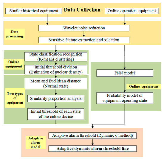
Figure 1.
The flowchart of method.
The specific calculation steps are as follows:
- (1)
- Process the historical device signal, including preprocessing and sensitive feature extraction.
- (2)
- Apply the K-means method to identify the operating state of the equipment and divide it into K operating states.
- (3)
- According to historical equipment data and kernel density estimation methods, obtain the thresholds of different states.
- (4)
- Collect dynamic data of online equipment and analyze the similar proportion between the data of the normal state of online equipment and historical equipment to obtain the initial alarm threshold for each state of the current equipment.
- (5)
- Input the data into the probabilistic neural network for analysis, construct the probabilistic model of the equipment state, and update the warning value according to the dynamic-σ update method to obtain the dynamic early warning lines at all levels of the equipment.
2.1. Pretreatment and Feature Extraction
Before clustering the original data, it is necessary to perform preprocessing, including data cleaning, noise reduction, and normalization. Data cleaning needs to identify and remove outliers and fill in missing values. Noise reduction aims to remove environmental noise in the data as much as possible and to smooth the data.
2.1.1. Wavelet Denoising
If a signal f(t) becomes s(t) after being polluted by noise, then the basic noise model can be expressed as:
where n(t) is noise and σ is the noise intensity. Wavelet denoising tries to attenuate the noise component n(t) so as to achieve the purpose of noise reduction.
In general, the wavelet denoising process of a one-dimensional signal can be divided into three steps as follows:
- (1)
- Wavelet decomposition of the signal: select the wavelet basis function, determine the appropriate number of wavelet decomposition layers, and then perform n-layer wavelet decomposition of the original signal s(t).
- (2)
- Threshold quantization of the wavelet decomposition coefficients: for the wavelet coefficients from the first layer to the Nth layer, the appropriate threshold is selected for threshold quantization.
- (3)
- Signal reconstruction by inverse wavelet transform.
The result of wavelet denoising depends on the following two points:
- (a)
- The denoised signal should have the same smoothness as the original signal, namely, the correlation ρ between the two columns of data should be high;
- (b)
- The smaller the root mean square error (RMSE) and the larger the signal to noise ratio (SNR) between the processed signal and the original signal are, the better the attained effect is.
The calculation equations of SNR, RMSE, and ρ for the evaluation indexes of noise reduction are as follows:
According to analysis of the steps of wavelet denoising, the types of wavelet bases, the number of decomposition layers, and the threshold quantization method all impact the final denoising effect. This paper also analyzes these three aspects and selects the most suitable wavelet denoising method.
2.1.2. Normalization
Because of the different dimensionality levels of the data, the larger-scale dimensional data will overwhelm the smaller-scale data and affect the clustering speed. To eliminate this effect, each variable needs to be normalized such that different variables can be analyzed and compared equally. The corresponding equation is as follows:
where qi is the measured value of the variable at the i-th moment, qmax is the maximum value of the variable in this period, qmin is the minimum value, and qiq is the normalized value.
2.1.3. Selection of Feature Variables
The extraction of feature variables has a direct impact on the accuracy and reliability of early fault warning. It is not better to select more fault features, and the increase in invalid features may lead to an increase in the complexity of the early warning process and a decrease in the accuracy of the diagnosis results. Therefore, it is necessary to select sensitive features that contain as much fault information as possible as input to the model. In this paper, the PCA-WLE method proposed in the literature [1] is adopted to extract and select sensitive features.
2.2. Operating State Identification
During the whole service life of the equipment, when it traverses the evolution process from normal to abnormal to the fault state, the historical data collected must include extensive data in the normal state, some data in the abnormal state, and little data in the fault state. Therefore, it is necessary to identify the different operating states of the equipment.
The K-means algorithm adopts the distance as the judgement index to divide the data set into K categories, based on the largest data difference among different categories and the highest degree of data similarity within the same category.
The historical data set is recorded as , wherein are the n data objects corresponding to n sensors; and the dimension of each group of data objects is N, i.e., . Let K be the number of cluster centres, and select K initial points as centroids, and the set of corresponding cluster centers is , for .
where is the number of points of the data object of category , and is the Euclidean distance between the centre of the category and the data object, which is used to measure the similarity between the data. The smaller the calculated value is, the greater the similarity is, which is defined as follows:
2.3. Threshold and Similarity Proportion of Each State
2.3.1. State Thresholds for Historical Equipment
According to the clustering results, the time series data in the different states of historical equipment can be obtained. The probability distribution of the different states and the corresponding state thresholds can also be obtained.
Kernel density estimation is a nonparametric probability density estimation method that is mainly applied to directly reflect the distribution of characteristic parameters of different states. In the actual production process, the probability density function of the collected data is often unknown, and the specific distribution form cannot be determined, so the kernel density estimation method is adopted to analyze the distribution law that is not known in advance. In this data processing approach, the data to be analysed are one-dimensional data, and the one-dimensional kernel density estimation equation is adopted:
where is the bandwidth for , and is a non-negative function called the kernel function. Here, the Gaussian function is used as the kernel function, namely, ; is the kernel density estimation of density function . Bandwidth H can be selected as the minimum of the mean integrated square error (MISE).
The initial threshold value of the alarm is defined as when the value of the probability distribution function reaches 99%.
2.3.2. Similar Proportion Function
For historical equipment and online equipment, although they operate under the same processing conditions and the external environment is basically the same, there will still be different degrees of deviation due to the component itself. To quantitatively express the deviations among the variables, a similar proportion function needs to be constructed to truly express the online devices.
In this paper, the Euclidean distance [34] between two groups of data and the mean are selected to construct a similar proportion function. The Euclidean distance between each data point can represent a similar proportion from the local point of view, while the mean represents the same from the overall point of view. The feature vector X obtained from the historical equipment and the feature vector Y obtained from the online equipment are selected for comparison.
where is the similar proportion function, is the distance similar proportion, and is the overall similar proportion. and are the distance weight and overall weight, respectively, and both belong to [0,1], for . and are the means of the historical and online equipment data, respectively. The larger the value is, the higher the similarity between the two is.
2.4. Dynamic Warning Lines at All Levels
2.4.1. State Probability Model of the Equipment
The online monitoring data are input into the probabilistic neural network for analysis, and the equipment state probability model is constructed according to the sum result. A probabilistic neural network is a neural network that can be used for pattern recognition based on the Bayesian minimum risk criterion. The calculation method of the conditional probability is mainly expressed by the Parzen method:
where is the sample vector to be identified, is the category, is the sample vector dimension, is the number of samples of category , is the training sample vector, and is the smoothing parameter. To simplify the model, the input feature indexes are all one-dimensional vectors, so the above equation can be simplified as follows:
where x is a feature of the state to be identified, N is the total number of training samples, and xi is the i-th training sample value.
2.4.2. Dynamic Adaptive Threshold Update Method
During the normal operation of the equipment, because of the change in field signal transmission and environment, the data are subject to constant dynamic fluctuations. The traditional fixed threshold method will cause false alarms or missing alarms, which will affect the early warning results. The dynamic-σ method is adopted to update the thresholds.
According to the Chebyshev inequality, the normal interval of any random variable with finite expectations and a finite variance is , where μ and σ are the mean and variance of the random variable, respectively, and the bandwidth coefficient is related to the error detection rate α, i.e., .
where zi is the measured value of the variable at the i-th moment. To reflect the dynamic nature of the data, it is necessary to input the data at each subsequent time point into the above equation for updating purposes. The mean value and variance are subsequently derived to further reduce the calculation amount and reduce the data storage space:
according to the calculation of the mean value and variance at time , only the mean value U and the variance Q at time and the measured value at time need be considered.
3. Experiment and Analysis Results
3.1. Experimental Data Description
With the full life cycle data of XJTU-SY rolling bearings as the test basis for analysis [35], the relevant parameters of the bearings are listed in Table 1. Two PCB-352C33 unidirectional acceleration sensors are fixed in the horizontal and vertical directions of the test bearing, and the DT9837 dynamic signal collector is applied to collect its vibration signal. The bearing test stand is shown in Figure 2. The bearing test platform can change the working conditions by adjusting the equipment parameters, including the rotational speed and radial force. An acceleration sensor is adopted to collect the vibration signal of the equipment. The sampling frequency is 25.6 kHz, the sampling interval is 1 min, and the sampling time is 1.28 s. Python was chosen as the software for writing and verifying the model in this article.

Table 1.
Tested bearing parameters.
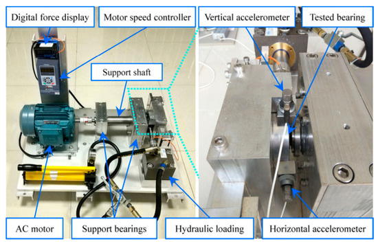
Figure 2.
Bearing test stand.
3.2. Analysis Results
The historical data of similar equipment under the working conditions of a rotational speed of 2100 r/min and radial force of 12 kN are selected for study, and the original vibration data are cleaned.
Different wavelet bases have different time-frequency characteristics, so different wavelets can obtain different results in denoising the same signal. Since a compact support and smoothness of the wavelet cannot be achieved at the same time, various factors must be considered comprehensively, and an eclectic method must be adopted to select the wavelet basis to better process the noisy signal. Thirty-seven kinds of commonly used wavelet bases are selected to reduce the noise of the signal, labelled 1–37, and the corresponding serial numbers are listed in Table 2. The signal to noise ratio (SNR), root mean square error (RMSE) and correlation coefficient of the noise-reduced signal are analyzed, as shown in Figure 3.
Table 2.
Commonly used wavelet bases and corresponding sequence numbers.
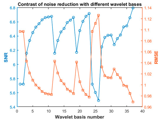
Figure 3.
Signal to noise ratio (SNR) and root mean square error (RMSE) of noise reduction for the different wavelet bases.
Generally, the higher the SNR of the signal is, the closer the noise reduction signal is to the energy of the real signal. The smaller the RMSE is, the smaller the deviation between the denoising signal and the actual signal is, the better the smoothness and denoising effect are. The closer the correlation coefficient is to 1, the better the similarity between the noise filtering signal waveform and the actual signal waveform is and the lower the distortion degree is. Through analysis of these 37 kinds of wavelets, it is found that the db10, sym8, coif5, and dmey wavelets attain better noise reduction effects on the signals used in this case.
The number of layers of wavelet decomposition also affect the noise reduction effect. The original signal is denoised by 2- to 8-layer wavelets, as shown in Figure 4. According to the analysis, when the number of decomposed layers is small, the SNR of the signal is high, the RMSE is small, and the correlation coefficient is high. Numerically speaking, the denoising effect is the best, but from the waveform point of view, the signal still contains much noise after denoising with a small number of layers. With the increase in the number of decomposition layers, the waveform of the denoising signal is smoother, but the distortion degree is higher. As shown in Table 3 and Figure 5, three layers are the optimal number of decomposition layers, which not only effectively eliminates noise but also retains the information in the signal as much as possible. Therefore, it is important to choose the number of decomposition layers properly to reduce noise when wavelet decomposition is performed.
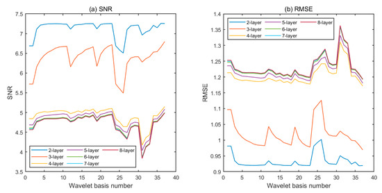
Figure 4.
SNR and RMSE of noise reduction with different decomposition layers.
Table 3.
SNR, RMSE, and correlation coefficient after the decomposition of different layers.
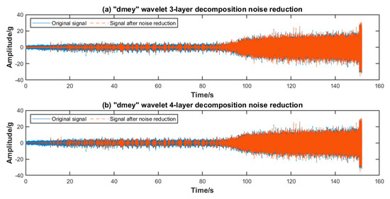
Figure 5.
The signal contrast between three and four layers after noise reduction.
The soft threshold, hard threshold, and fixed threshold are also compared and analyzed, as summarized in Table 4. Four kinds of wavelet basis functions are adopted to reduce noise, among which the hard threshold method is the best, the fixed threshold method attains the second best effect, and the soft threshold method performs the worst. Finally, the hard threshold denoising method of dmey wavelet 3-layer decomposition is applied to denoise the signal.
Table 4.
SNR and RMSE of the four wavelet bases after noise reduction with three layers.
A total of 52 features are extracted from the noise-reduced signal, as shown in Table 5. Among them, wavelet packet energy and energy entropy are decomposed through dmey wavelet 4-layer decomposition. According to the PCA-WLE [1] feature selection method, the root mean square value RMS, wavelet packet total energy ET and node 1 wavelet packet energy entropy S1 are selected as sensitive features. Meanwhile, the obtained features are normalized. The RMS of the signal can describe the vibration energy and reflect the wear degree of the bearings, while the wavelet packet energy and its entropy have a high noise resistance, and the higher the energy in the sub-band is, the more notable the fault information is.
Table 5.
Relevant features of bearings.
The running state of the bearings is divided into four types: normal operation, mild anomaly, moderate anomaly, and severe anomaly, namely, K = 4. With the selected sensitive features as clustering parameters, according to the historical data, the K-means clustering method is applied to obtain the clustering centre of the operating conditions, as summarized in Table 6. The results of K-means clustering are shown in Figure 6.
Table 6.
Historical data clustering centres and thresholds.
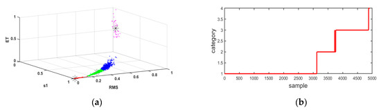
Figure 6.
Results of k-means clustering analysis: (a) spatial representation of clustering results; (b) temporal variation of different categories.
The kernel density of the fault data in the four states is estimated, and the corresponding probability distribution diagram is obtained. When the value of the probability distribution function reaches 99%, it is used as the initial alarm threshold to realize early warning. The results are shown in Figure 7, and the initial threshold is summarized in Table 6. The part above the threshold of the severe anomaly is considered to be in the state of complete failure.
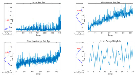
Figure 7.
Probability distribution diagram.
Then, the vibration signal of the online running bearings is collected. The experiment is performed at a speed of 2100 r/min and a radial force of 12 kN. The time series data of the online running bearings in the normal running state are , and n is the number of data points in the sampling period. The normal data of the historical equipment and online equipment in the same time period are selected for similar proportion analysis, and the Euclidean distance and cluster centre of the two sets are calculated.
Through correlation calculation, the similarity proportions are and . The distance weight and center weight are both set to 0.5. Finally, the similarity ratio is obtained. Based on this ratio, the initial thresholds of the different states of the online devices under the same working environment conditions can be derived, as listed in Table 7.
Table 7.
The initial threshold of the online equipment in each state.
The online monitoring data are input into the one-dimensional probabilistic neural network model, from which the probabilistic neural network can establish the probabilistic model of the running state of the equipment. According to the calculation method of the dynamic early warning value mentioned above, the data of each additional 10 cycles (i.e., 8000 sampling points) are input into the model for updating purposes, and each alarm value is linked to obtain dynamic early warning lines at all levels, as shown in Figure 8a.
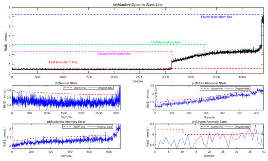
Figure 8.
Adaptive dynamic alarm line in each state of the equipment.
Selecting the normal state data as an example, Figure 9 shows the early warning method based on a fixed threshold [36] and the early warning line of the early warning method proposed in this paper. It is clear that the warning line obtained with the warning method based on the fixed threshold will clearly cause many over-limit alarms. However, the dynamic adaptive early warning line can adjust the threshold value fittingly according to the environment fluctuation when the data do not produce large anomalies, which can greatly reduce the number of false positives. From the dynamic warning diagram, it is evident that the dynamic warning lines at all levels can regulate the operation range of the equipment in the different health states. When the detection features exceed a certain range, the current equipment has deviated from its existing state. Field staff can further process the equipment according to its state, such as strengthening monitoring or directly shutting down for maintenance. When the detection features fluctuate above and below the threshold line or even drop, the equipment is considered to be in the unstable state, which is the run-in period rather than a fault. When the detection features exceed the level-4 warning line and keep rising, the equipment is considered to be in the fault state and needs to be shut down for maintenance in this case.
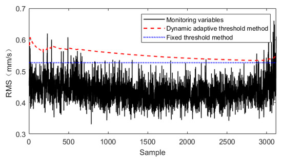
Figure 9.
Comparison of the different threshold methods (normal state).
For the two methods, the result when the actual value exceeds the warning line is recorded as 1 at a certain time and as 0 below the warning line. The result is shown in Figure 10. Through comparative analysis of the two methods in Figure 10a,b, it can be seen that for the normal state data, both early warning methods exhibit over-limit behavior in the early stage, but the data quickly recede, indicating that at this time, only data fluctuation occurs within the normal range. The data after the 3000th instance are considered to be developing toward the abnormal state, namely, it is regarded as the correct early warning behaviour for any method. Before the 3000th instance, the method based on the fixed threshold issued 69 false alarms, while the method based on dynamic adaptive warning only issued 7 false alarms, indicating that the latter greatly reduced the number of false alarms in the online detection of equipment.
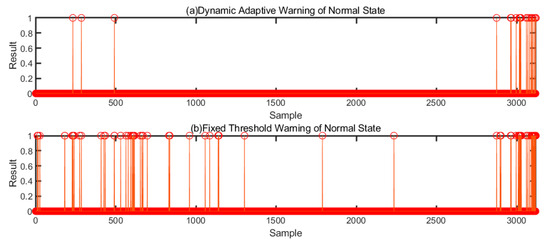
Figure 10.
Warning results based on the different threshold methods.
Based on the dynamic adaptive early warning method, after the equipment leaves the abnormal state, it can make adaptive adjustments for the different abnormal states and issue early warnings for the more serious abnormal states or even complete faults in the next stage, providing more detailed guidance and maintenance strategies for the field staff.
4. Conclusions
This paper introduces a new flexible multi-state adaptive early warning method for mechanical equipment and proposes an adaptive dynamic update model of the equipment alarm threshold based on the similar proportion and state probability model. In the case of early warning of rolling bearings, this method is compared to the traditional fixed threshold method, which verifies the superiority of this method. According to the experimental and analytical results, the following conclusions can be drawn:
- Based on the similarity of historical equipment, the initial thresholds of the different health states of online equipment can be determined, which can intuitively reflect the current state of the equipment, provide an early warning of sudden failures, and offer a certain reference guidance for online equipment under the same working conditions.
- The monitoring data of online equipment change with the interference of external factors such as environment and working conditions, and when the equipment is in the abnormal state, its abnormal degree changes accordingly. In this paper, the equipment status is divided into four categories and analyzed, which can better represent its status and provide more detailed and reasonable guidance.
- The obtained dynamic alarm lines at all levels can regulate the operation range of the equipment in its different health states, which makes the method proposed in this paper not only attain a high sensitivity by alarming when abnormal or even when a fault occurs in the equipment but can also tolerate the data fluctuation caused by the equipment in the run-in period to a certain extent to prevent false positives.
- Compared to the traditional method of a fixed threshold, this method can effectively reduce the number of false alarms and realizes a higher prediction accuracy, which demonstrates its effectiveness and superiority.
The early warning of online equipment from the perspective of the similar probability and proportion model can be applied not only to bearing monitoring but also to the early warning of other online equipment. However, there are still many unsolved problems that need to be addressed in future research, such as how to determine the failure type during maintenance based on early warning of the equipment and how to settle data volatility and intervals in data updating.
Author Contributions
W.D., W.Z., and T.H. conceived the methodology. Y.L. established the model and performed the simulations. W.D. and Y.L. wrote and edited the manuscript. W.D., M.S., and T.H. revised and polished the manuscript. All authors have read and agreed to the published version of the manuscript.
Funding
The authors acknowledge the financial support of the National Natural Science Foundation of China (No. 51705015), the Fundamental Research Foundation (No. JCKY2018203C005), and the Technical Foundation Program (No. JSZL2019601A003) from the Ministry of Industry and Information Technology of China.
Conflicts of Interest
The authors declare no conflict of interest.
References
- Li, Y.; Dai, W.; Zhang, W. Bearing Fault Feature Selection Method Based on Weighted Multidimensional Feature Fusion. IEEE Access 2020, 8, 19008–19025. [Google Scholar] [CrossRef]
- Yazhou, L.; Wei, D.; Dongmei, S.; Weifang, Z. Reliability Evaluation of Rolling Bearing Based on Wavelet Packet Energy Entropy. In Proceedings of the Prognostics and System Health Management Conference (PHM-Qingdao), Qingdao, China, 25–27 October 2019; pp. 1–6. [Google Scholar]
- Lv, Y.; Fang, F.; Yang, T.; Romero, C.E. An early fault detection method for induced draft fans based on MSET with informative memory matrix selection. ISA Trans. 2020, 102, 325–334. [Google Scholar] [CrossRef] [PubMed]
- Cui, C.; Lin, W.; Yang, Y.; Kuang, X.; Xiao, Y. A novel fault measure and early warning system for air compressor. Measurement 2019, 135, 593–605. [Google Scholar] [CrossRef]
- Braglia, M.; Bevilacqua, M. The analytic hierarchy process applied to maintenance strategy selection. Reliab. Eng. Syst. Saf. 2000, 70, 71–83. [Google Scholar]
- Dhumale, R.B.; Lokhande, S.D. Neural Network Fault Diagnosis of Voltage Source Inverter under variable load conditions at different frequencies. Measurement 2016, 91, 565–575. [Google Scholar] [CrossRef]
- Liang, L.; Liu, F.; Li, M.; He, K.; Xu, G. Feature selection for machine fault diagnosis using clustering of non-negation matrix factorization. Measurement 2016, 94, 295–305. [Google Scholar] [CrossRef]
- Du, W.; Zhou, W. An Intelligent Fault Diagnosis Architecture for Electrical Fused Magnesia Furnace Using Sound Spectrum Submanifold Analysis. IEEE Trans. Instrum. Meas. 2018, 67, 2014–2023. [Google Scholar] [CrossRef]
- Jiang, G.; Xie, P.; He, H.; Yan, J. Multiscale Convolutional Neural Networks for Fault Diagnosis of Wind Turbine Gearbox. IEEE Trans. Ind. Electron. 2019, 66, 3196–3207. [Google Scholar] [CrossRef]
- Glowacz, A. Fault diagnosis of single-phase induction motor based on acoustic signals. Mech. Syst. Signal Process. 2019, 117, 65–80. [Google Scholar] [CrossRef]
- Glowacz, A.; Glowacz, W.; Glowacz, Z.; Kozik, J. Early fault diagnosis of bearing and stator faults of the single-phase induction motor using acoustic signals. Measurement 2018, 113, 1–9. [Google Scholar] [CrossRef]
- Lu, C.; Wang, Z.; Zhou, B. Intelligent fault diagnosis of rolling bearing using hierarchical convolutional network based health state classification. Adv. Eng. Inf. 2017, 32, 139–151. [Google Scholar] [CrossRef]
- Ramos, A.R.; Llanes-Santiago, O.; Bernal De Lazaro, J.M.; Corona, C.C.; Neto, A.J.S.; Galdeano, J.L.V. A novel fault diagnosis scheme applying fuzzy clustering algorithms. Appl. Soft Comput. 2017, 58, 605–619. [Google Scholar] [CrossRef]
- Jiang, W.; Hu, W.; Xie, C. A New Engine Fault Diagnosis Method Based on Multi-Sensor Data Fusion. Appl. Sci. 2017, 7, 280. [Google Scholar] [CrossRef]
- Yonggang, X.; Zhang, K.; Ma, C.; Li, X.; Zhang, J. An Improved Empirical Wavelet Transform and Its Applications in Rolling Bearing Fault Diagnosis. Appl. Sci. 2018, 8, 2352. [Google Scholar]
- Chen, X.; Wang, P.; Hao, Y.; Zhao, M. Evidential KNN-based condition monitoring and early warning method with applications in power plant. Neurocomputing 2018, 315, 18–32. [Google Scholar] [CrossRef]
- Zhu, P.; Qian, H.; Chai, T. Research on early fault warning system of coal mills based on the combination of thermodynamics and data mining. Trans. Inst. Meas. Control 2020, 42, 55–68. [Google Scholar] [CrossRef]
- Martínez-Sibaja, A.; Astorga-Zaragoza, C.M.; Alvarado-Lassman, A.; Posada-Gómez, R.; Aguila-Rodríguez, G.; Rodríguez-Jarquin, J.P.; Adam-Medina, M. Simplified interval observer scheme: A new approach for fault diagnosis in instruments. Sensors 2011, 11, 612–622. [Google Scholar] [CrossRef]
- Zhu, P.X.; Jin, G.Y.; Yan, Y.Q.; Gao, S.Y. Fault Diagnosis of Rolling Bearing Based on Improved Independent Component Analysis and Cepstrum Theory. Adv. Mater. Res. 2013, 2731, 188–192. [Google Scholar] [CrossRef]
- Orsagh, R.; Roemer, M.; Sheldon, J.; Klenke, C.J. A comprehensive prognostics approach for predicting gas turbine engine bearing life. In Proceedings of the ASME Turbo Expo 2004:Power for Land, Sea and Air, Vienna, Austria, 14–17 June 2004; pp. 777–785. [Google Scholar]
- Meng, Z.; Shi, G.; Wang, F. Vibration response and fault characteristics analysis of gear based on time-varying mesh stiffness. Mech. Mach. Theory 2020, 148, 103786. [Google Scholar] [CrossRef]
- Widarsson, B.; Dotzauer, E. Bayesian network-based early-warning for leakage in recovery boilers. Appl. Therm. Eng. 2008, 28, 754–760. [Google Scholar] [CrossRef]
- Yao, Y.; Wang, N. Fault diagnosis model of adaptive miniature circuit breaker based on fractal theory and probabilistic neural network. Mech. Syst. Signal Process. 2020, 142, 106772. [Google Scholar] [CrossRef]
- Gupta, S.; Kambli, R.; Wagh, S.; Kazi, F. Support-Vector-Machine-Based Proactive Cascade Prediction in Smart Grid Using Probabilistic Framework. IEEE Trans. Ind. Electron. 2015, 62, 2478–2486. [Google Scholar] [CrossRef]
- Zhou, Q.; Xiong, T.; Wang, M.; Xiang, C.; Xu, Q. Diagnosis and Early Warning of Wind Turbine Faults Based on Cluster Analysis Theory and Modified ANFIS. Energies 2017, 10, 898. [Google Scholar] [CrossRef]
- Zhang, W.; Liu, J.; Gao, M.; Pan, C.; Huusom, J.K. A fault early warning method for auxiliary equipment based on multivariate state estimation technique and sliding window similarity. Comput. Ind. 2019, 107, 67–80. [Google Scholar] [CrossRef]
- Guo, P.; Infield, D.; Yang, X. Wind Turbine Generator Condition-Monitoring Using Temperature Trend Analysis. IEEE Trans. Sustain. Energy. 2012, 3, 124–133. [Google Scholar] [CrossRef]
- Peng, J.; Zhou, Z.; Wang, J.; Wu, D.; Guo, Y. Residual Remaining Useful Life Prediction Method for Lithium-Ion Batteries in Satellite With Incomplete Healthy Historical Data. IEEE Access 2019, 7, 127788–127799. [Google Scholar] [CrossRef]
- Fang, F.; Romero, C.E.; Lv, Y.; Li, J.; Yang, T. Typical condition library construction for the development of data-driven models in power plants. Appl. Therm. Eng. 2018, 143, 160–171. [Google Scholar]
- Soualhi, A.; Medjaher, K.; Celrc, G.; Razik, H. Prediction of bearing failures by the analysis of the time series. Mech. Syst. Signal Process. 2020, 139, 106607. [Google Scholar] [CrossRef]
- Rostek, K.; Morytko, L.; Jankowska, A. Early detection and prediction of leaks in fluidized-bed boilers using artificial neural networks. Energy 2015, 89, 914–923. [Google Scholar] [CrossRef]
- Wang, J.; Xiong, X.; Zhou, N.; Li, Z.; Wang, W. Early warning method for transmission line galloping based on SVM and AdaBoost bi-level classifiers. IET Gener. Trans. Distrib. 2016, 10, 3499–3507. [Google Scholar] [CrossRef]
- Feng, T.; Bi, J.; Yuan, H. Real-time and short-term anomaly detection for GWAC light curves. Comput. Ind. 2018, 97, 76–84. [Google Scholar]
- Alencar, J.; Bonates, T.; Lavor, C.; Liberti, L. An algorithm for realizing Euclidean distance matrices. Electron. Notes Discret. Math. 2015, 50, 397–402. [Google Scholar] [CrossRef]
- Wang, B.; Lei, Y.; Li, N.; Li, N. A Hybrid Prognostics Approach for Estimating Remaining Useful Life of Rolling Element Bearings. IEEE Trans. Reliab. 2020, 69, 401–412. [Google Scholar] [CrossRef]
- Quan, Z.; Sheng, F.; Jing, L. Application of Wavelet Package and Neural Network in Ventilators Fault Warning. In Proceedings of the International Conference on Condition Monitoring & Diagnosis, Beijing, China, 21–24 April 2008; pp. 1362–1364. [Google Scholar]
© 2020 by the authors. Licensee MDPI, Basel, Switzerland. This article is an open access article distributed under the terms and conditions of the Creative Commons Attribution (CC BY) license (http://creativecommons.org/licenses/by/4.0/).