Next Article in Journal
Combination of Different Approaches to Infer Local or Regional Contributions to PM2.5 Burdens in Graz, Austria
Next Article in Special Issue
Erratum: Heilmeier, A., et al. Application of Monte Carlo Methods to Consider Probabilistic Effects in a Race Simulation for Circuit Motorsport. Appl. Sci. 2020, 10, 4229
Previous Article in Journal
Numerical Analysis of Multi-Phase Flow around Supercavitating Body at Various Cavitator Angle of Attack and Ventilation Mass Flux
Previous Article in Special Issue
Innovative Approaches in Sports Science—Lexicon-Based Sentiment Analysis as a Tool to Analyze Sports-Related Twitter Communication
 
 
Erratum published on 19 August 2020, see Appl. Sci. 2020, 10(17), 5745.
Article

Application of Monte Carlo Methods to Consider Probabilistic Effects in a Race Simulation for Circuit Motorsport

1
Institute of Automotive Technology, Technical University of Munich, 85748 Garching, Germany
2
BMW Motorsport, 80939 Munich, Germany
*
Author to whom correspondence should be addressed.
Appl. Sci. 2020, 10(12), 4229; https://doi.org/10.3390/app10124229
Submission received: 11 May 2020 / Revised: 3 June 2020 / Accepted: 15 June 2020 / Published: 19 June 2020
(This article belongs to the Collection Computer Science in Sport)

Abstract

:
Applying an optimal race strategy is a decisive factor in achieving the best possible result in a motorsport race. This mainly implies timing the pit stops perfectly and choosing the optimal tire compounds. Strategy engineers use race simulations to assess the effects of different strategic decisions (e.g., early vs. late pit stop) on the race result before and during a race. However, in reality, races rarely run as planned and are often decided by random events, for example, accidents that cause safety car phases. Besides, the course of a race is affected by many smaller probabilistic influences, for example, variability in the lap times. Consequently, these events and influences should be modeled within the race simulation if real races are to be simulated, and a robust race strategy is to be determined. Therefore, this paper presents how state of the art and new approaches can be combined to modeling the most important probabilistic influences on motorsport races—accidents and failures, full course yellow and safety car phases, the drivers’ starting performance, and variability in lap times and pit stop durations. The modeling is done using customized probability distributions as well as a novel “ghost” car approach, which allows the realistic consideration of the effect of safety cars within the race simulation. The interaction of all influences is evaluated based on the Monte Carlo method. The results demonstrate the validity of the models and show how Monte Carlo simulation enables assessing the robustness of race strategies. Knowing the robustness improves the basis for a reasonable determination of race strategies by strategy engineers.

1. Introduction

Motorsport races are competitions held to determine a ranking among the participants. In circuit races, the result depends not only on the driver and car performance but also on race strategy. Since the participants of such races drive a certain number of laps on a closed circuit, they can drive into their pits at the end of every lap. Pit stops are mostly taken in order to obtain a fresh set of tires, allowing the driver to drive a faster lap time than with an old set. However, since pit stops take some time, one must find an effective compromise between benefit and expanse. These aspects are determined by race strategy.
Race simulations are used to simulate and compare the effects of different race strategies. The common approach to building such simulations is to discretize the race lap-wise, as we presented in an earlier paper [1]. Thus, the first simulation step in every lap l is to calculate the expected lap times t lap of the drivers. To obtain them, the simulation adds up a number of different time parts in a lap time model, as shown in Equation (1) [1]. t base is the lap time that the fastest car-driver combination can theoretically achieve in the race, that is, when the tires are fresh and the car has almost no fuel on board. It therefore takes into account the characteristics of the race track. To this basis are added: t tire for the effect of tire degradation (dependent on tire age a tire and compound c tire ), t fuel for the time lost due to the fuel mass that is carried in the car, t car and t driver for the car and driver abilities, t grid for the time that is lost at the race start (dependent on grid position p g ) and t pit , in - lap / out - lap for the time that is lost in pit stops [1].
t lap ( l ) = t base + t tire ( a tire , c tire ) + t fuel ( l ) + t car + t driver + t grid ( l , p g ) + t pit , in - lap / out - lap ( l )
Consecutive lap times of a driver are summed up to obtain his race times t race at the end of every lap as given by [1]
t race ( l ) = i = 1 l t lap ( i ) .
The race times are the central element of the simulation. For example, they can be compared in order to determine whether an overtaking maneuver would have taken place in reality. This will be the case if the calculated race time of the pursuer is sufficiently smaller (i.e., faster) than that of the car in front. Figure 1 visualizes the simulation flow chart. The strategy engineer specifies the participants’ strategies and obtains their race durations (and therefore also their final rank positions).
The lap-wise discretization provides a good compromise between computational effort, parameterization effort, and accurate results. Although it causes some modeling difficulties, as will be discussed later, it is preferred over other approaches because the fast computing times are essential for the intended application. They enable the strategy engineer to quickly compare the results of many different strategies before and during a race. Moreover, they make the application of the Monte Carlo method, and thus the ideas presented in this paper, possible in the first place. For comparison: A time-discrete simulation or a simulation of the individual driving lines of every car would be orders of magnitude slower and would be hard to parameterize.
In the presented state, however, the simulation misses one crucial aspect: real races are often decided by random events. If, for example, a driver causes an accident, race control usually sends a safety car on the track. Among other things, it significantly reduces the race speed while the crashed car is removed from the track, which leads to increased lap times. Consequently, probabilistic events such as this should be modeled within the race simulation to allow the strategy engineer to determine a stable race strategy. “Stable” in this context means that the strategy should be robust against unforeseen events, that is, it should have a high probability on the targeted rank position.

2. Related Work

The literature and also this paper concentrate on the FIA Formula 1 World Championship because it is the most popular circuit racing series, and accordingly, most data is available. Nevertheless, the presented ideas could be adapted to other racing series as well.
For the determination of the simulation parameters, as well as for the analysis of the probabilistic influences in this paper, a comprehensive database is required. In our case, it is based on the Ergast API [2], which is a web service that hosts Formula 1 timing data. It provides us, for example, with lap times, positions, and pit stop durations. We restructured and extended the data for our purpose, for example, by adding information on accidents and failures, safety car and virtual safety car phases, and the tire compounds used. Furthermore, several cross-checks are carried out during the creation of the database, for example, that the tire compound only changes during a pit stop. Our database covers the Formula 1 hybrid era, that is, the seasons from 2014–2019. It is available under an open-source license on GitHub (https://github.com/TUMFTM/f1-timing-database).
Little literature is available that deals with race simulations, and especially the modeling of probabilistic effects in this context. The published works on this topic are based on the Monte Carlo simulation (MCS) concept. MCS “uses random sampling to study properties of systems with components that behave in a random fashion” [3] p. 1. The result of interest for a strategy engineer is the final rank position of his driver. Therefore, MCS is applied by implementing realistic models for the probabilistic effects and then simulating a huge amount of races to determine the estimated distribution of the rank positions. Table 1 gives an overview of the literature coverage on this topic as well as an evaluation of the presented models. The evaluation is based on an assessment of the completeness and accuracy of the models. The models and evaluations are explained in more detail in the next paragraphs.

2.1. Starting Performance

“Starting performance” in this context means the driver’s performance at the start of the race. A good starter will, on average, gain positions during the race start. This can be modeled by sampling the number of lost or gained positions at the race start from an empirical distribution based on historical data [4,7]. The sampled changes are then applied to the drivers’ positions. The problem with this approach is that the positions are changed without changing the respective lap times accordingly, which is not realistic. Furthermore, the treatment of edge cases is unclear. For example, how should it be handled if the driver on the third grid position should win two positions, and the driver on the second grid position should win one position?
Another possibility is used by Phillips [5] and Salminen [6]. They convert the driver-specific average number of positions lost or gained in the first lap p change , start ¯ into a positive or negative delta time. The result is used as the mean μ startperf of a Gauss distribution, cp. Equation (3). The corresponding standard deviation σ startperf is set 0.25 s [6] or 1 s [5]. In the first lap, the distribution is sampled to obtain t startperf for every driver, see Equation (4). It can be considered in t grid , which was introduced in Equation (1).
μ startperf = p change , start ¯ · 0.25 s
t startperf N μ startperf , σ startperf 2
Our criticism of this variant is that using the average number of gained and lost positions per driver distorts the probabilities. For example, Lewis Hamilton (world champion in 2018) lost, on average, 0.8 positions in the first laps of the 2018 races, whereas Lance Stroll (ranked 18 of 20 in 2018) gained 1.9 positions [8]. There are several such examples. This is because drivers starting mostly in front positions have only a small potential to improve their position compared to drivers starting at the back of the starting grid. Additionally, the used values for σ startperf are not based on data.

2.2. Variability of Lap Time and Pit Stop Duration

When analyzing real lap times, it can be observed that they are scattered around a mean value, since no driver can perfectly repeat a lap. For the analysis of this effect, other influences on the lap times have to be removed as far as possible, for example, the effects of tire degradation and burned fuel mass. Therefore, quadratic polynomials of the form t lap , poly ( l ) = k 2 l 2 + k 1 l + k 0 are fitted to the real lap times t lap for every stint. This is visualized in the upper part of Figure 2. Since we only want to include “clean” laps, the first two laps (heavily affected by the start of the race) and all laps that are affected by pit stops or full course yellow (FCY) phases have to be removed from the process. FCY phases are used by race control to reduce speed when there is danger on the race track.
The driver-specific lap time deviations t lap , dev shown in the lower part of Figure 2 can then be calculated by
t lap , dev ( l ) = t lap ( l ) t lap , poly ( l ) .
The deviations are approximately normally distributed. Accordingly, Sulsters [7], Phillips [5] and Salminen [6] model the lap time variability by adding a sample t lap , var from a Gauss distribution with zero mean and driver-specific standard deviation (cp. Equation (6)) to every lap time t lap in Equation (1).
t lap , var N 0 , σ lap , var 2
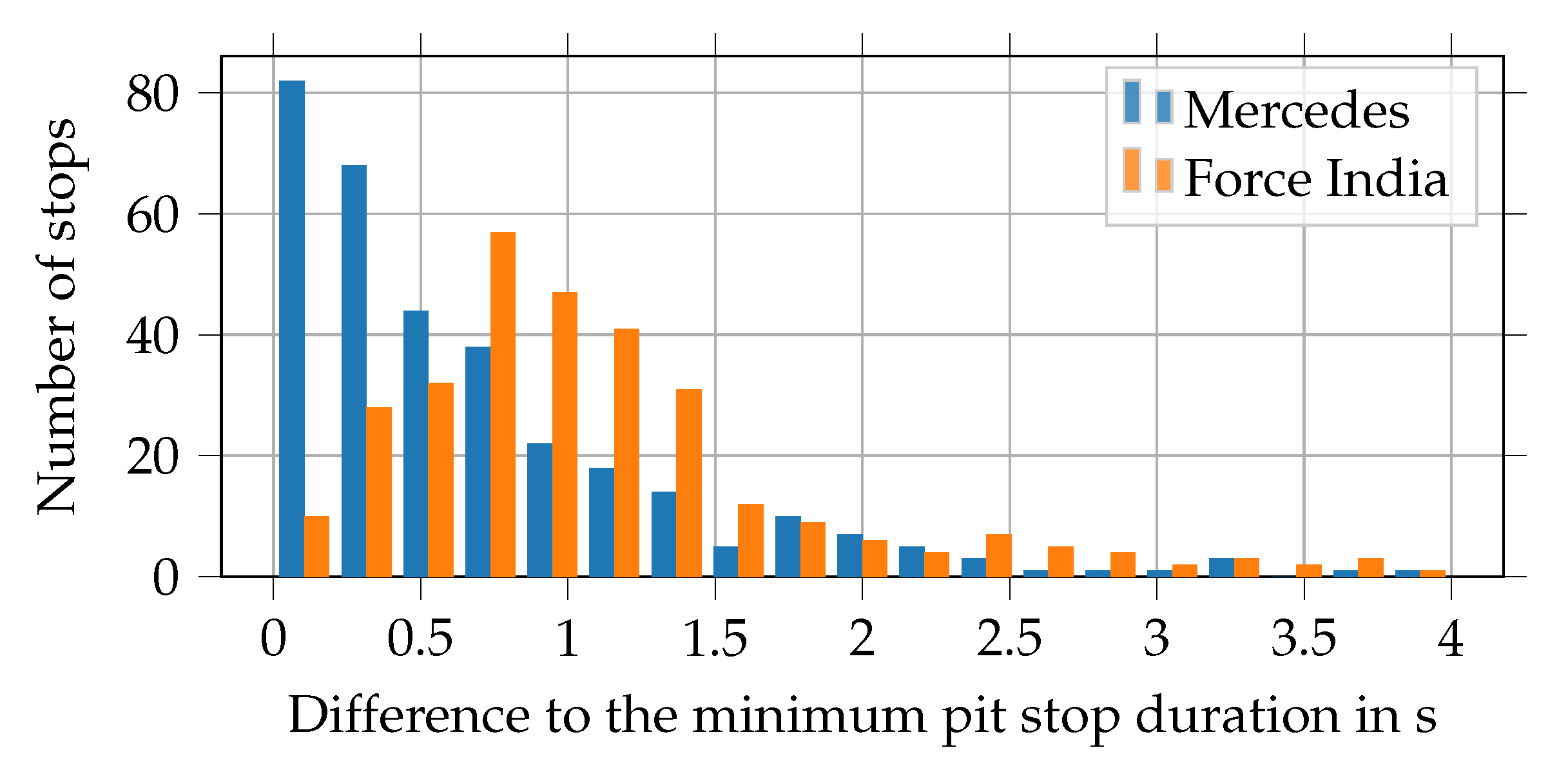
As can be seen in Figure 3, pit stop durations vary as well. The plot indicates that the pit stop durations of Mercedes are mostly very close to the minimum duration of the races, whereas Force India’s pit stops often take significantly longer.
The data demonstrate that a symmetric Gauss distribution would not fit for modeling this variability. Therefore, Phillips [5] uses a log-logistic distribution, also known as Fisk distribution F , to model this effect, cp. Equation (7). The distribution is fitted individually for every team using the three parameters s h a p e , l o c , and s c a l e [9]. A sample from the distribution is then added to t pit , in - lap / out - lap of Equation (1) when a driver performs a pit stop. Bekker et al. [4] state that they included the effect, but do not describe it any further.
t pit , var F s h a p e , l o c , s c a l e

2.3. Accidents and Failures

Accidents and (technical) failures both result in the driver being unable to continue the race, known as “did not finish” (DNF) or “retirement”. In literature, no distinction is drawn between the two causes. Bekker et al. [4] use driver-specific probabilities P dnf to determine in every lap if a driver retires. Phillips [5] and Salminen [6] extend the driver-specific probabilities by a lap dependency to consider that there are significantly more retirements during the first lap than in other laps. This results from the small distances between the drivers shortly after the start of the race.
All the probabilities P dnf are based on the fraction of real DNFs of a driver. Consequently, they would be derived to an unrealistic zero if a driver did not have a DNF within the scope of the database. Table 2 demonstrates that this is the case with Lewis Hamilton in the 2019 season, for example. Sulsters [7], therefore, uses Bayesian inference to transfer the knowledge from all available DNFs in the database to the particular driver to determine if he retires within a race. As a result, even drivers without a DNF get a (low) probability for retirement. The approach seems promising. However, Sulsters [7] also does not differentiate between accidents and failures, although both causes affect the races differently, as will be shown later.

2.4. Damaged Car

In contrast to cars that retire due to an accident or failure, a damaged car can continue the race. Salminen [6] is the only author to modeling this case. He introduces a 1% damage chance per overtaking maneuver for each of the involved cars, and another 1% that both are damaged. A uniform distribution models the effect of damage according to Equation (8). Besides, damaged cars perform an immediate pit stop at the end of the lap.
t damage U 2 s , 60 s
The problem with modeling damaged cars is that a lot of detailed data is required to consider them correctly, especially the relationship between damage, accidents, and FCY phases. To our knowledge, this data is not available to the public. Since Salminen [6] does not describe where the values come from, the modeling of the effect seems unclear.

2.5. Full Course Yellow Phases

A regular yellow flag indicates minor danger in a sector of the race track, for example, a slow car. The effect on the race is negligible. Full course yellow phases indicate a significant danger and therefore have a bigger impact. They limit the speed of the drivers, which increases the lap times. In Formula 1, FCY phases are differentiated into virtual safety car (VSC) and safety car (SC) phases. The race control decides, depending on the danger for the race participants and marshals, which variant is deployed. A VSC prescribes a minimum lap time t lap , vsc for every driver. Figure 4 indicates, that t lap , vsc is about 140% of the fastest unaffected lap time of a race t lap , min . Since every driver has to keep to it immediately, the time intervals between the drivers remain more or less constant. During an SC phase, drivers must also reduce their speed, similar to a VSC phase. Additionally, a physical car drives out of the pit lane onto the race track in front of the race leader. It drives much slower than the race cars and must not be overtaken. Therefore, it increases the lap times further to t lap , sc 1.6 · t lap , min as soon as the drivers reach it on the track, cp. Figure 4. As a result, the gaps between the drivers vanish. A crucial element for race strategy is that the relative time loss for driving through the pit lane is significantly reduced during VSC and SC phases since it depends on how long it takes to pass the pit lane on the race track in comparison to driving through it. Under SC or VSC conditions, the cars drive slower on the track while driving through the pit lane is always speed limited and, therefore, not affected.
It can be seen in Figure 4 that the lap times vary considerably during SC and VSC phases. Therefore, when calculating the average lap time increases mentioned in the previous paragraph, we apply the following criteria in order to consider only representative lap times. For SC phases, we use those laps in which the SC has already been on track for more than 1.5 laps before the lap and which are not the last lap of the phase. For VSC phases, the lap must be fully covered by the phase. Generally, only the lap times of the drivers on positions 1–3 are used. The values are averaged over all seasons 2014–2019.
Sulsters [7] models an SC by increasing the lap time of every driver for five laps by 20%. Phillips [5] simulates SC phases for six laps. He distinguishes between run-up phase (20% lap time increase) and following phase (40% lap time increase). Additionally, he reduces tire wear during an SC phase. Salminen [6] is the only author distinguishing between VSC and SC phases. The VSC is modeled by a lap time increase of 20%. The SC implementation is similar to Phillips [5] except for the reduced tire wear, which is neglected. However, Salminen [6] takes into account the reduced time loss of pit stops during FCY phases t pit , in - lap / out - lap , fcy :
t pit , in - lap / out - lap , fcy = 0.5 · t pit , in - lap / out - lap .
When comparing the implementations in the literature with reality, it becomes clear that several aspects are not modeled accurately. Firstly, FCY phases in the presented approaches always start and end exactly on a completed lap, which is not the case in reality. Secondly, in reality, VSC and SC always appear at the same point in race time t race for every driver, which is different from appearing at certain race progress, especially if some slower drivers are lapped during the race. For example, if an SC is deployed in lap 30, it starts when the race leader is in lap 30. A lapped driver, in contrast, would already be affected in lap 29 in reality. Therefore, it makes more sense to simulate the SC start at a specified race time, for example, t race = 3000 s , instead of a specified race progress as in literature. Thus, it affects the race of every driver as it would in reality. Thirdly, according to our assessment of the data, t lap , vsc and t lap , sc are much bigger than what is assumed in literature. Fourthly, the time loss of pit stops under FCY conditions t pit , in - lap / out - lap , fcy is highly dependent on the race track layout and cannot simply be halved. Since this is an important element of race strategy, it should be parameterized more accurately.

3. Methodology

With the lap-wise discretized race simulation (described in Section 1) as a basis, there are few alternatives to MCS for evaluating the effects of probabilistic influences. One option would be to use what-if scenarios, for example, “What happens if the SC gets deployed on lap 30?”. However, this can only be dealt with if we refrain from considering combinations of many probabilistic influences due to the rapidly increasing complexity. Another idea would be to discretize the possible range of the random variables and then simulate races for all combinations (full factorial design). In contrast to MCS, this approach would lead to better sampling of the parameter space in low-probability regions. MCS, on the other hand, provides more meaningful results because it utilizes probability distributions that represent real behavior. Besides, a full factorial design suffers from the curse of dimensionality, which quickly increases computation time. As in literature, MCS is therefore preferred. MCS requires that the generated random numbers are independent and identically distributed [3] p. 4. Provided that the computer’s random number generator (RNG) fulfills this requirement, it also holds for most of the commonly used random distributions, since they are sampled based on the RNG. This also applies to the distributions used in this paper: Gauss distribution [11], Beta distribution [12] and log-logistic (Fisk) distribution [12].
The following sections describe how we have modeled the influences presented in the previous chapter in order to overcome the mentioned limitations. Damaged cars are not considered as we do not have the necessary data available. Besides, it is a rare case that a car that has been involved in an accident is only damaged so slightly that it can continue the race.

3.1. Modeling of Starting Performance

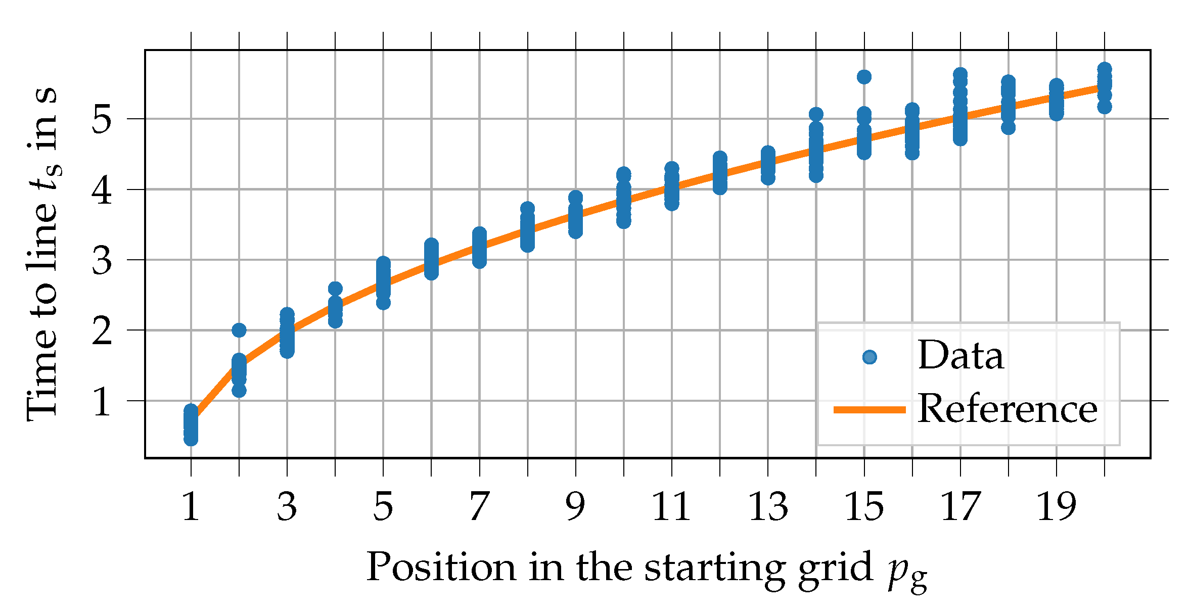
To be able to distinguish between good and bad starters, we need a reference, that is, an average starter. Therefore, we measured the times between race start and crossing the start line (in front of the starting grid) t s as a function of starting grid position p g for the 2019 races. This was done using videos from the cockpit perspective, which are available on F1 TV [13]. As Figure 5 reveals, a square root function is a good approximation of the average starter.
The square root function is physically rational if we assume a constant acceleration for the race start phase. This hypothesis can be made because Formula 1 cars are grip limited and not power limited in the lower speed range. The function is established as follows:
t s = 2 ( p g p s ) a avg + t r .
The parameters p s and t r stand for the (virtual) position of the start line and the reaction time of a human driver. They shift the origin so that a driver who would start directly on the start line would only have to overcome his reaction time. p s is set 0.8 because the start line is located only slightly in front of the pole position. Therefore, the distance to the pole starter is significantly smaller than the usual distance between two grid positions (which is 8 m ). As a consequence, p s cannot be set 0. For the reaction time t r we use 0.2 s . The average acceleration during the race start a avg is then determined using a least-square fit. This results in a avg = 11.2 m / s 2 when evaluating the data of the 2019 season as shown in Figure 5 and using the distance of 8 m between two starting grid positions.
With the parameterized reference curve, as depicted in Figure 5, we can calculate the differences to the measured data points for every driver. These deviations are then used to calculate mean and standard deviation of a driver-specific Gauss distribution, which is used to modeling the starting performance t startperf as stated by Equation (4). Samples from these distributions are added to the first lap time in the race simulation. The parameters of the drivers of the 2019 season can be found in Table A1 in Appendix A.

3.2. Modeling of Variability of Lap Time and Pit Stop Duration

The modeling of the variability of lap time and pit stop duration is adapted from literature as presented in Equations (6) and (7). However, the parameterization was carried out on our significantly larger database. The parameters of the drivers and teams of the 2019 season are given in the Table A1 and Table A2 in Appendix A.

3.3. Determination of Accident and Failure Probabilities

As mentioned, we want to differentiate between accidents and (technical) failures. Therefore, we assume that an accident depends on the driver, while a failure depends on the car, that is, the team. If a team changed its name from one season to the next, for example, when Sauber became Alfa Romeo Racing, we treat it under its original name to ensure that the failure probabilities are determined correctly. The accident and failure probabilities are determined by applying Bayesian inference, as suggested by Sulsters [7]. For Bayesian inference, a prior distribution and a likelihood function are required. As with Sulsters [7], the Beta distribution is used as prior distribution, and the Bernoulli distribution as likelihood function (the possible race outcomes are: “finished” or “did not finish”). The prior distribution parameters α ^ and β ^ are determined to [7] p. 11
α ^ = 1 μ ^ σ ^ 2 1 μ ^ μ ^ 2 and
β ^ = α ^ 1 μ ^ 1 .
μ ^ and σ ^ stand for mean and standard deviation of the prior distribution. They are determined using the total accident fraction per driver, and the total failure fraction per team. Hereby, only drivers and teams with at least 30 races in the database are considered. The two prior distributions for accidents and failures then represent our knowledge about the respective probabilities on the entire database.
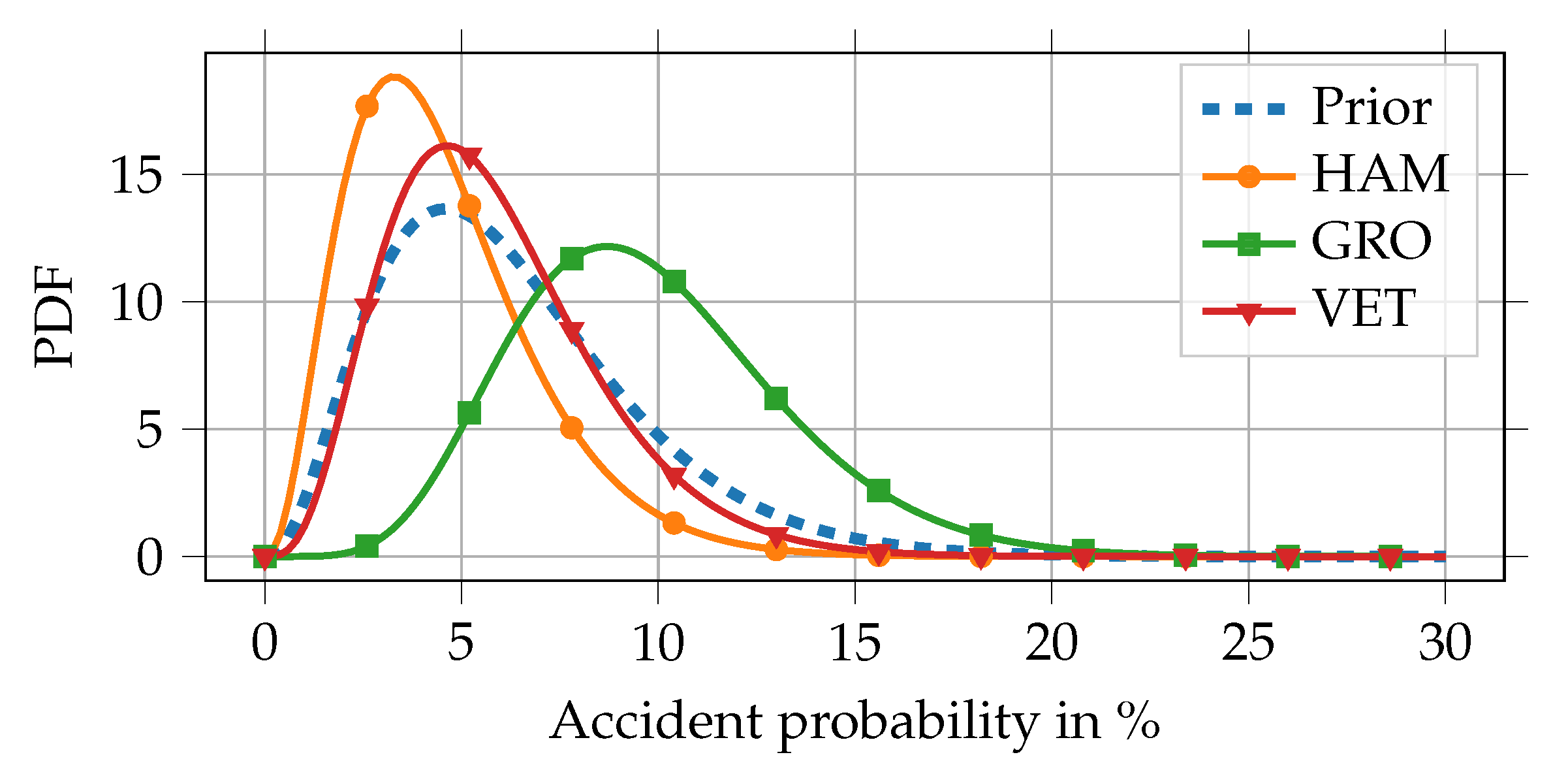
Thereafter, driver-, team- and season-specific posterior distributions are calculated taking into account the corresponding accident and failure fractions within the particular season. This proceeding combines the overall knowledge with the specific influence factors of driver, team, and season. For the chosen combination of prior distribution and likelihood function, the posterior distributions are also a Beta ( α + z , β + N z ) distribution [7] p. 12. z is the number of accidents or failures in the respective season, and N stands for the number of attended races in that season. Figure 6 shows the resulting probability density functions of the accident prior distribution and three driver-specific accident posterior distributions.
Finally, the mean values of the posterior distributions are used as accident P accident and failure probabilities P failure for the simulation. The parameters of the drivers and teams of the 2019 season are given in the Table A1 and Table A2 in Appendix A.

3.4. Determination of Full Course Yellow Phases in Combination with Accidents and Failures

The determination of FCY phases and retirements must be performed before starting the actual race simulation in order to have the required information available even if backward drivers reach the specified start of a phase in an earlier lap than the race leader. The alternative would be to determine the retirements and their corresponding FCY phases “live” during the simulated race, as used in some of the literature. A small example shows why this does not work correctly with the lap-wise discretization principle. Looking at exemplary race times in Table 3, we find that driver 1 is ahead of driver 2 and driver 3 in laps 20–22 because he reaches the end of each lap earlier (actually driver 3 was even lapped because t race (driver 1, lap 21) < t race (driver 3, lap 20)). Assuming that the simulation would decide in lap 22 that a VSC phase should be activated at t race = 2110 s , we can conclude that it would affect driver 1 shortly after starting into lap 22, while driver 2 and driver 3 would have already been affected in lap 21. Therefore, the problem is that once the simulation decides to activate the VSC phase in lap 22, the previous lap has already been fully simulated due to lap-wise discretization. As a consequence, the SC could not be considered for driver 2 and driver 3 in lap 21 anymore.
The solution is to determine all FCY phases and retirements before starting the actual race simulation, as explained in the following. For the definition of FCY phases, a process to fix start race times, durations, and type (VSC or SC) is required. The definition must happen in conjunction with the determination of accidents and failures since they are the causes of FCY phases. For our process, we assume that accidents lead to SC phases. In contrast, if a driver retires due to a failure, he tries to drive to a safe spot. Therefore, we assume that this either causes a VSC phase or no FCY phase at all. We use the following procedure to keep the overall chances of SC, VSC, accidents, and retirements as realistic as possible, although it violates the real cause-effect principle in the case of SC phases:
  • Determine SC phases (quantity, start, duration) and derive accidents
  • Determine failures (quantity, start) and derive VSC phases (duration)
  • Convert race progress to race time
Determine SC phases and derive accidents
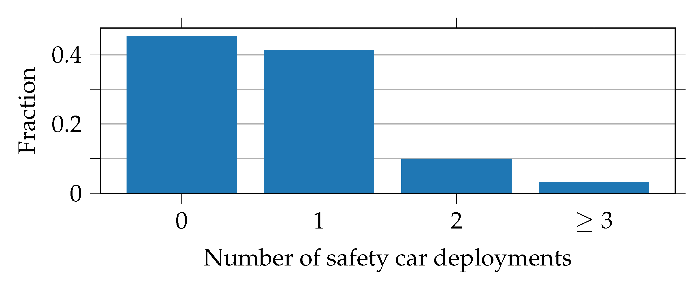
The SC phases are fixed at first because they have a significant impact on race strategy, and therefore their probability of occurrence should be no conditional probability. The quantity of SC phases for a race is chosen between zero and three, whereby empirical probabilities P sc , quant according to the real fractions of the seasons 2014–2019 are used for each of the options, see Figure 7. The exact values are given in Table A3 in Appendix A.
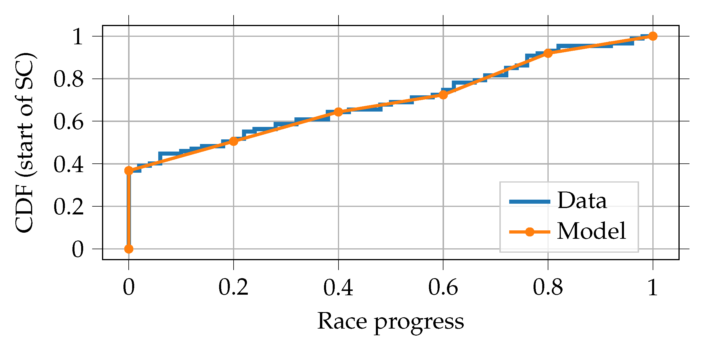
Then, the start of every SC phase is defined. Therefore, the race is divided into six groupings (first lap, 20 % , 40 % , 60 % , 80 % , 100 % ) with individual probabilities P sc , start . The laps in each group are then assigned the same proportion of the corresponding probability. This classification can be compared with the actual data in Figure 8. The exact values for P sc , start are given in Table A4 in Appendix A. The first lap has to be considered separately since over 36 % of the SC phases start here, which can be explained by the small distances between the drivers shortly after the start that cause a high probability of accidents.
The duration of an SC phase is chosen to be between two and eight laps with empirical probabilities P sc , duration derived from data of the seasons 2014–2019. The exact values are given in Table 4. The start of an SC phase is further modified by a uniform distribution U ( 0 , 1 ) to include the fact that it does not start precisely at the point laps are completed.
Before finally saving the created phase, it is assured that it does not overlap an already existing phase. This would be the case if
r fcy , s , n r fcy , e , e + r fcy , d and
r fcy , s , e r fcy , d r fcy , e , n
both hold. r fcy , s / e , n is the race progress at the start and end of the new and r fcy , s / e , e the race progress at the start and end of the existing FCY phase currently in comparison. r fcy , d is a minimum distance which should be kept between two phases.
As mentioned before, we assume that every SC phase is caused by an accident. Therefore, the simulation chooses one driver who retires at the start of every SC phase. The selection happens based on the drivers’ accident probabilities P accident that were determined earlier. Selecting only a single driver for an accident is a simplification, since sometimes two or even more drivers are involved in reality. However, our available data is not detailed enough to be able to modeling and parameterize these cases. Furthermore, retired drivers are not crucial for race strategy determination.
Determine failures and derive VSC phases
Thereafter, the simulation determines, for those drivers not involved in an accident, whether they suffer a failure. The team-specific failure probability P failure determined earlier is used in this respect. Subsequently, the simulation checks for every failure appearing if it causes a VSC phase using the conditional probability P ( vsc | failure ) . Assuming that every VSC is caused by a failure, it can be calculated using the number of VSC phases n vsc and the number of failures n failures (2015–2019, as the VSC was introduced in 2015) in the database:
P ( vsc | failure ) = n vsc n failures = 0.227 .
This is a simplification because there are some cases where, after an accident, VSC phases were first activated and shortly afterward replaced by an SC phase, for example. However, as before, the available data is not detailed enough to analyze these cases. The start of the failure (and probably of the phase) is sampled from a uniform distribution U ( 0 , n laps ) since no outstanding race section could be identified in the data. n laps stands for the number of laps in the race. The duration of a possible VSC phase is chosen in the range between one and four laps, with empirical probabilities P vsc , duration , and modified by a uniform distribution U ( 0 , 1 ) as with the start of SC phases. The exact probabilities for the duration determination are given in Table 5.
Convert race progress to race time
Due to the lap-based nature of the information in the database, the definition of FCY phases and retirements is also based on laps (i.e., race progress). However, as mentioned in Section 2.5, race times are required instead of race progress so that every driver can be affected at the same point in time. This is achieved by converting the race progress information into race times using a pre-simulation of the actual race with a single driver. It gives a reasonable estimate at which race time a particular stage of progress is reached during the race. Thus, the progress information of the FCY phases can be converted to race times. Deviations between the race times of the pre-simulation and the real race simulation cause no problems, as they change the start and duration of the phases equally for every driver.

3.5. Modeling of Accidents, Failures, and Full Course Yellow Phases

The modeling of accidents and failures is implemented by simply taking the concerned driver out of the race as soon as his race time exceeds the defined time of retirement.
Modeling of the virtual safety car
The VSC is modeled by increasing the lap times of the drivers to t lap , vsc = 1.4 · t base , cp. Section 2.5. However, since FCY phases can start and end at any point during a lap, we have to calculate the lap fractions that are driven normally f n and affected by the VSC phase f vsc to obtain the correct lap time. If, for example, the phase starts within the current lap and ends in a later lap, the resulting lap time t lap can be calculated by
f n = t race , vsc , s t race , l - 1 t lap , n ,
f vsc = 1.0 f n , and
t lap = f n · t lap , n + f vsc · t lap , vsc ,
where t race , vsc , s is the start race time of the VSC phase, t race , l - 1 the race time of the driver at the end of the previous lap and t lap , n the unaffected lap time of the driver in the current lap. Similar calculations are performed when the phase ends. Overtaking is forbidden in the simulation if a VSC affects at least 50% of a lap. Due to the limited speed, tire degradation and fuel consumption are reduced to 50% during the phase. This is an estimation since the exact values cannot be derived from the publicly available data. In reality, the saved fuel is, of course, consumed after the phase, for example, by increasing the engine power. In the simulation, the average consumption per lap after an FCY phase is therefore automatically adjusted so that the saved fuel is used up by the race finish.
Modeling of the safety car
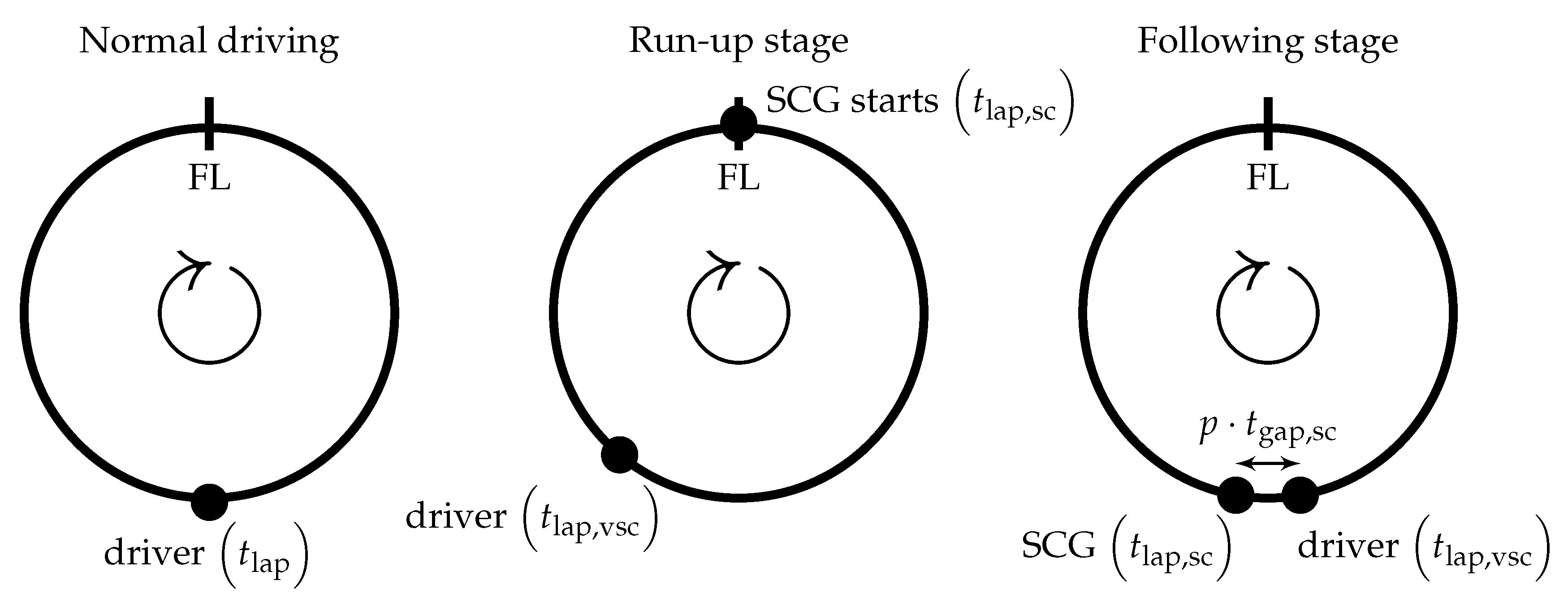
For the realistic modeling of SCs, we use driver-individual “safety car ghosts” (SCGs). The concept is illustrated in Figure 9. An SCG can be imagined as a virtual car that is only visible to its corresponding driver and does not affect any other driver. Since it is a safety car, it cannot be overtaken. The driver-individual handling is necessary, since the drivers may be affected by the same SC in different laps due to lap-wise discretization. An SC deployment is modeled in two stages, a run-up stage and a following stage. If a driver reaches the start race time of an SC phase, we assume that his SCG starts driving on the finish line exactly at this time. Equally to the VSC, the lap time of the respective driver is then increased up to t lap , vsc for the remaining part of the lap and following laps to simulate the run-up stage under full course yellow condition. Every driver catches up with his SCG within several laps, since it drives at 160% of the base lap time, cp. Section 2.5. The first SCG lap time is even slower to modeling the real behavior where the SC waits for the leading driver at the pit exit. If a driver’s calculated race time at the end of a lap is below that of his SCG, he would have overtaken it. Thus his lap time is artificially increased to stay behind. Keeping a minimum temporal spacing t gap , sc between the drivers is hereby assured by adding p · t gap , sc to the individual SCG race times, where p stands for the drivers’ rank positions. Tire degradation and fuel consumption are reduced to 25% (again an estimation) while driving behind an SC. The value is smaller than that of the VSC phase because the speed is even lower. The SCGs remain active until the end of the lap in which the SC phase ends, even if the originally determined end time is reached before the end of the lap. This models the fact that the SC can only leave the race track by entering the pit lane at the end of a lap. This proceeding allows a realistic simulation of the re-start of the race with small gaps between the drivers. After each SC phase, the drag reduction system (DRS) is deactivated for two laps, as in reality. The DRS allows drivers to reduce drag resistance on straights when following another driver at a close range. It was introduced in the 2011 season to ease overtaking.
Adjustment of pit time losses under FCY condition
As mentioned, it is crucial to consider that the relative pit time loss t pit , in - lap / out - lap reduces if a driver drives through the pit lane during an FCY phase. Therefore, smaller pit time losses are added if entering or leaving the pit is fully covered by an FCY phase. During an SC phase, the time losses are often even smaller than during a VSC phase. Since the data are not publicly available, we measured them using videos from the cockpit perspective in 2018 and 2019, which are available on F1 TV [13]. As Table 6 indicates, the differences between normal conditions and FCY conditions vary largely depending on the track layout. Substitute values (for t pit , in - lap / out - lap , vsc and t pit , in - lap / out - lap , sc ) from similar tracks can be used for race tracks for which no VSC or SC phases have been declared in 2018 and 2019.

4. Results

The race simulation is implemented in Python. The computation time for a race with 20 participants (as in the 2019 season) is 90 m s –110 m s on a common computer (Intel i7-6820HQ) including the pre-simulation. For MCS, the races can be simulated independently from each other. Therefore, the calculation time benefits from multiple CPU cores almost linearly. This allows us to perform 10 , 000 simulation runs in about 250 s to 300 s using all four cores of the CPU.
For reasons of clarity, only the six drivers of the three currently dominating teams (Mercedes, Ferrari, Red Bull) are simulated and shown in this section.

4.1. Effect of Full Course Yellow Phases

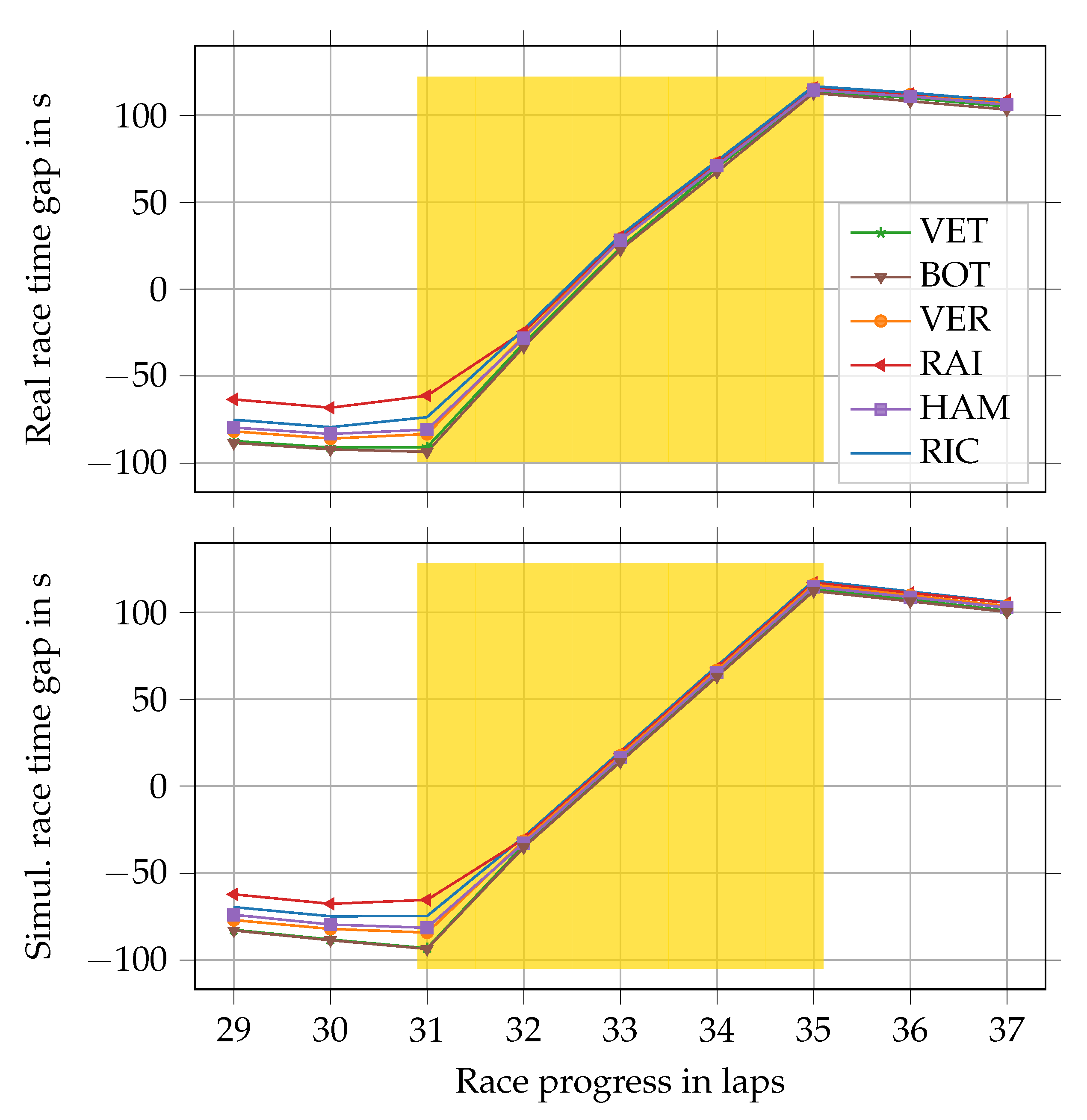
Figure 10 shows a comparison between real and simulated race time gaps for laps 29 to 37 of the 2018 Chinese Grand Prix. The gaps t race , gap are calculated by subtracting the lap-wise race times of a virtual driver from those of the real drivers, cp. Equation (19). The lap time of the virtual driver t lap , virt is constant and chosen so that his total race duration corresponds to that of the race winner, as given by Equation (20). The plot then clearly visualizes where the drivers gain (negative gradient) and lose (positive gradient) time during the race in comparison to the average lap time. The yellow boxes in the figure mark the laps affected by an SC phase. For this example, the phase was set to fit the real race in the simulation.
t race , gap ( l ) = t race ( l ) l · t lap , virt
t lap , virt = t race , winner n laps
The figure demonstrates a good correspondence between real and simulated data. As in reality, drivers approach the SC in the simulation and follow it with the corresponding lap time. As can be seen from the small gradient, lap 31 is only slightly affected by the SC in simulation and reality because the SC gets deployed very late in that lap. In this example, all six drivers catch up with the SC within lap 32 because they were not far apart before the SC deployment. Accordingly, they simply follow the SC in laps 32–35. The figure also proves that the re-start of the race happens similarly in simulation and reality in lap 36.

4.2. Analysis of Monte Carlo Simulations

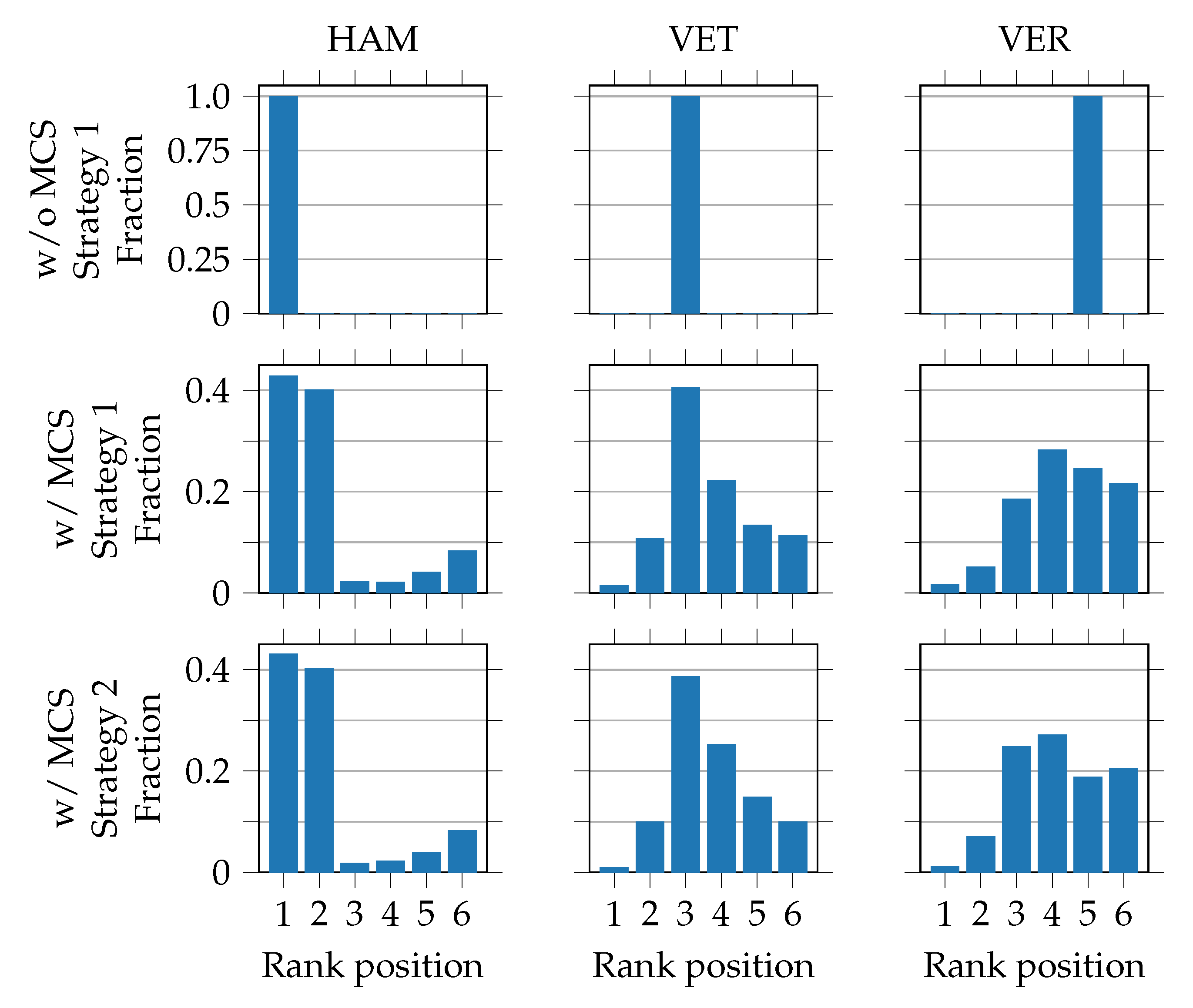
Figure 11 presents an exemplary MCS output for three of the six drivers. The plots show the fraction of races that the drivers have completed on the respective positions. They tell us about the expected race outcome with a given race strategy, which can be used to evaluate different variants. The first row in the figure (w/o MCS) displays the deterministic simulation output, that is, without using MCS. The second and third rows (w/MCS) show the resulting position distributions for two different race strategies for Verstappen when using MCS. In this example, Verstappen’s pit stop was postponed from lap 14 (strategy 1) to lap 19 (strategy 2).
We want to point out three aspects of the figure. Firstly, the second row provides much more information than the first row because MCS was applied. For Verstappen, for example, it turns out that fifth place in the race is only the second most likely outcome, although the deterministic simulation shows this as a result. For Hamilton, it is almost as likely to finish second as it is to finish first. Secondly, we can observe a shift in the position distribution of Verstappen when switching from strategy 1 to strategy 2. It results in an improvement in third positions. This would again not have been visible in the deterministic simulation. Similar investigations can also be carried out with different tire compounds, for example. Thirdly, the fraction of rank position six is slightly above the previous ones for Hamilton. Retirements due to accidents and failures explain this.
Hence, MCS allows us to determine a basic race strategy before a race that already considers probabilistic influences. At the same time, we gain an idea of the robustness of the strategy against unforeseen events because it is fixed, that is, not adapted to the race situation during the simulation. During a real race, of course, this basic strategy must be adapted to the current situation, for example, SC phases. Without MCS, we would only obtain a single result, which is much less helpful for strategy determination.
It is not only final positions that can be evaluated with the combination of race simulation and MCS. Figure 12 depicts the distribution of race durations after 10,000 simulation runs for this exemplary race. The durations of races without an SC phase differ only slightly. The widely distributed hill between 95 min to 103 min indicates races with a single SC phase. Races with two and three SC phases also have a high spread but appear relatively seldom.
However, the fraction of SC phases in the simulation fits well with the actual data. This is outlined in Table 7. The VSC fractions differ slightly due to the conditional probability depending on previous failures, cp. Equation (15).
But how reliable is the MCS result after, for example, 10,000 simulation runs? According to the law of large numbers, it approaches the expectation ever more closely, the more often the random experiment is repeated. Table 8 shows an evaluation of Hamilton’s mean rank position in an exemplary race after 20 batches of simulation runs. It can be seen that the deviation between the batches decreases with a rising number of simulation runs per batch. This behavior is similar for all drivers. In most cases, 10,000 simulation runs offer a good compromise between computation time and certainty. However, it must be emphasized that the result of the race itself depends strongly on a correct parameterization of the race simulation.

5. Discussion

As shown in Section 4.2, the results of the deterministic race simulation do not indicate that they often do not represent the most likely outcome of a race. Additionally, the theoretically fastest strategy for a race often turns out to be fragile when probabilistic effects are considered. Consequently, race simulations should include these effects, which can be evaluated using MCS. Thus, the strategy engineer can benefit from information on the position distribution and robustness of different race strategies against unforeseen events.
The significance of the MCS results depends on the accurate modeling of the probabilistic influences. Therefore, we extended existing ideas (e.g., using Bayesian inference for accidents and failures) and developed new approaches (determination of FCY phases, modeling of safety cars, starting performance) to improve on the points criticized in the literature. Of note is the FCY phase implementation, which affects the drivers equally regardless of their respective race progress. The SCG concept allows the realistic modeling of safety cars despite the lap-wise discretization. The example in the results section outlines that the approach represents reality well. The separate consideration of accidents and failures increases model accuracy and strengthens the cause-effect relationship with the FCY phases. Finally, the presented model for the starting performance does not distort probabilities for drivers starting predominantly at the front or back of the starting grid. The database with the seasons 2014–2019 allows a significantly improved and extended parameterization compared to the literature.
There are, however, some inaccuracies. In reality, at the end of an SC phase, lapped drivers may often catch up one lap to restore the correct ranking of the drivers for the re-start. This behavior cannot be simulated due to lap-wise discretization. For the same cause, an SC in the simulation does not start directly in front of the leader, but at a particular race time. However, this disadvantage was largely eliminated by increasing the first SCG lap time, so that the drivers quickly catch up with their SCG. Another inaccuracy is that we can currently only consider one driver per accident that causes an SC phase. This could be eliminated if more detailed data were available, which would allow us to analyze accidents involving several cars. A thorough analysis of the conditional probability for VSC phases after failures would also be desirable in that case.
The computing time of the race simulation was kept at a similar level despite the extensions. For obtaining the results of Monte Carlo simulations even faster, the introduction of Latin Hypercube sampling could be investigated in the future. Presumably, this reduces the number of simulation runs required to achieve a defined maximal deviation. Regarding our future research, we aim to focus on the optimization of race strategy using the developed race simulation. The challenge is that the basic strategy before a race cannot be determined independently for a single team since every team aims for an optimum. Consequently, the mutual effects must be taken into account. Furthermore, during a race, the basic strategy needs to be quickly adapted to the current race situation, for example, in the case of an SC. This requires a solution that can provide the results very quickly.

6. Summary

In this paper, we presented several new approaches and extensions to modeling important probabilistic effects on a motorsport race within a lap-wise discretized race simulation. This includes driver-specific starting performance, accident and failure probabilities, as well as the determination of full course yellow phases and the modeling of safety cars. The displayed results illustrate the validity of the SC model and show how a strategy engineer can benefit from evaluating probabilistic effects using Monte Carlo simulation when determining race strategies.
The entire Python code of the race simulation is available under an open-source license on GitHub (https://github.com/TUMFTM/race-simulation).

Author Contributions

A.H., as the first author, developed most of the presented approaches and extensions, implemented them in the race simulation, and performed large parts of the data analysis to obtain the required parameters. M.G., as the mentor of the research project, critically scrutinized the approaches. M.G., J.B., and M.L. contributed to the conception of the research project and revised the paper critically. Conceptualization, A.H., M.G., J.B.; data curation, A.H.; formal analysis, A.H.; methodology, A.H.; software, A.H.; validation, A.H.; writing–original draft preparation, A.H.; writing–review and editing, A.H.; visualization, A.H.; supervision, M.G., J.B. and M.L. All authors have read and agreed to the published version of the manuscript.

Funding

Research was supported by the basic research fund of the Institute of Automotive Technology of the Technical University of Munich.

Acknowledgments

We want to acknowledge Marcel Faist, who worked on the automated parameterization of the race simulation during his master’s thesis within the research project. He initiated the idea for the modeling of the starting performance based on a reference curve (the establishment of the square root function in the presented form was carried out by A.H.). Besides, he carried out all measurements using the videos from the cockpit perspective on F1 TV [13].

Conflicts of Interest

The authors declare no conflict of interest.

Abbreviations

The following abbreviations are used in this manuscript:
CDFCumulative Distribution Function
DNFDid Not Finish
DRSDrag Reduction System
FCYFull Course Yellow
MCSMonte Carlo Simulation
PDFProbability Density Function
RNGRandom Number Generator
SCSafety Car
SCGSafety Car Ghost
VSCVirtual Safety Car

Appendix A. Parameterization of the Probabilistic Effects in the Race Simulation

Table A1. Driver-specific parameterization for accident probability P accident , lap time variability t lap , var and starting performance t startperf for all drivers of the 2019 season. P accident is season-specific, the other values are valid for all seasons 2014–2019.
Driver P accident (2019) t lap , var in s N μ , σ 2 t startperf in s N μ , σ 2
Alexander Albon0.045 N 0 , 0.628 2 N 0.050 , 0.168 2
Antonio Giovinazzi0.058 N 0 , 0.737 2 N 0.006 , 0.148 2
Carlos Sainz Jnr0.045 N 0 , 0.606 2 N 0.097 , 0.126 2
Charles Leclerc0.058 N 0 , 0.533 2 N 0.042 , 0.125 2
Daniel Ricciardo0.058 N 0 , 0.517 2 N 0.047 , 0.112 2
Daniil Kvyat0.058 N 0 , 0.586 2 N 0.027 , 0.146 2
George Russell0.072 N 0 , 0.759 2 N 0.044 , 0.174 2
Kevin Magnussen0.058 N 0 , 0.608 2 N 0.014 , 0.171 2
Kimi Raikkonen0.058 N 0 , 0.499 2 N 0.088 , 0.245 2
Lance Stroll0.058 N 0 , 0.642 2 N 0.095 , 0.135 2
Lando Norris0.058 N 0 , 0.603 2 N 0.003 , 0.142 2
Lewis Hamilton0.045 N 0 , 0.459 2 N 0.052 , 0.098 2
Max Verstappen0.058 N 0 , 0.473 2 N 0.001 , 0.171 2
Nico Hulkenberg0.058 N 0 , 0.548 2 N 0.027 , 0.115 2
Pierre Gasly0.045 N 0 , 0.591 2 N 0.044 , 0.154 2
Robert Kubica0.045 N 0 , 0.841 2 N 0.029 , 0.128 2
Romain Grosjean0.072 N 0 , 0.612 2 N 0.102 , 0.156 2
Sebastian Vettel0.045 N 0 , 0.458 2 N 0.050 , 0.115 2
Sergio Perez0.058 N 0 , 0.550 2 N 0.009 , 0.152 2
Valtteri Bottas0.058 N 0 , 0.482 2 N 0.028 , 0.135 2
Table A2. Team-specific parameterization for failure probability P failure and pit stop duration variability t pit , var for all teams of the 2019 season. P failure is season-specific, t pit , var is valid for all seasons 2014–2019. The parameterization of the pit stop duration variability is based on pit stop durations that are at most 4 s longer than the minimum pit stop duration of a race.
Team P failure (2019) t pit , var in s ( F (shape, loc, scale))
AlfaRomeo0.056 F ( 5.827 , 0.953 , 2.327 )
Ferrari0.086 F ( 2.414 , 0.153 , 0.737 )
HaasF1Team0.101 F ( 5.324 , 0.667 , 1.866 )
McLaren0.117 F ( 2.639 , 0.235 , 0.980 )
Mercedes0.041 F ( 1.563 , 0.046 , 0.480 )
RacingPoint0.056 F ( 3.498 , 0.249 , 1.188 )
RedBull0.071 F ( 2.045 , 0.094 , 0.598 )
Renault0.086 F ( 3.876 , 0.419 , 1.433 )
ToroRosso0.071 F ( 4.290 , 0.568 , 1.606 )
Williams0.071 F ( 2.562 , 0.240 , 0.966 )
Table A3. Probabilities for a specified quantity of safety car (SC) deployments in a race (seasons 2014–2019).
Probability0 SC1 SC2 SC 3 SC
P sc , quant 0.4550.4130.0990.033
Table A4. Probabilities for the start of a safety car phase in one of the six groupings of the race (seasons 2014–2019). The probability of each grouping is divided equally among the laps in it, depending on the total number of laps in the respective race.
Probability1st Lap2nd Lap to 20%20 to 40%40 to 60%60 to 80%80 to 100%
P sc , start 0.3640.1360.1360.080.1930.091

References

  1. Heilmeier, A.; Graf, M.; Lienkamp, M. A Race Simulation for Strategy Decisions in Circuit Motorsports. In Proceedings of the 2018 21st International Conference on Intelligent Transportation Systems (ITSC), Maui, HI, USA, 4–7 November 2018; pp. 2986–2993. [Google Scholar] [CrossRef]
  2. Newell, C. Ergast Motor Racing Developer API. Available online: http://ergast.com/mrd (accessed on 8 May 2020).
  3. Lemieux, C. Monte Carlo and Quasi-Monte Carlo Sampling; Springer Series in Statistics; Springer: New York, NY, USA, 2009. [Google Scholar] [CrossRef] [Green Version]
  4. Bekker, J.; Lotz, W. Planning Formula One race strategies using discrete-event simulation. J. Oper. Res. Soc. 2009, 60, 952–961. [Google Scholar] [CrossRef]
  5. Phillips, A. Building a Race Simulator. Available online: https://f1metrics.wordpress.com/2014/10/03/building-a-race-simulator (accessed on 8 May 2020).
  6. Salminen, T. Race Simulator: Downloadable R Program Code. Available online: https://f1strategyblog.wordpress.com/2019/05/10/race-simulator-downloadable-r-program-code (accessed on 8 May 2020).
  7. Sulsters, C. Simulating Formula One Race Strategies. Master’s Thesis, Vrije Universiteit Amsterdam, Amsterdam, The Netherland, 2018. [Google Scholar]
  8. Collantine Media Ltd. RaceFans Race Data 2018. Available online: https://www.racefans.net/2018-f1-season/2018-f1-statistics/2018-f1-race-data (accessed on 8 May 2020).
  9. The SciPy Community. Documentation on scipy.stats.fisk. Available online: https://docs.scipy.org/doc/scipy/reference/generated/scipy.stats.fisk.html (accessed on 29 May 2020).
  10. Collantine Media Ltd. RaceFans Retirements Data 2019. Available online: https://www.racefans.net/2019-f1-season/2019-f1-statistics/2019-f1-retirements-penalties (accessed on 29 May 2020).
  11. Box, G.E.P.; Muller, M.E. A Note on the Generation of Random Normal Deviates. Ann. Math. Stat. 1958, 29, 610–611. [Google Scholar] [CrossRef]
  12. Leemis, L. Document Page of the Math Department of the College of William & Mary. Available online: http://www.math.wm.edu/~leemis/chart/UDR/PDFs (accessed on 8 May 2020).
  13. Formula One Digital Media Limited. F1 TV. Available online: https://f1tv.formula1.com (accessed on 29 May 2020).
Figure 1. Flow chart of a lap-wise discretized race simulation (based on the flow chart presented in [1]). The block “probabilistic effects” contains most of the extensions proposed in this paper.
Applsci 10 04229 g001
Figure 2. Visualization of the lap time variability of Hamilton in Austin 2019. The deviations are the difference between real lap times and a quadratic polynomial fitted separately for every stint. The first two laps, as well as laps affected by pit stops or full course yellow phases, are not included in this process.
Applsci 10 04229 g002
Figure 3. Histogram plot showing the differences between the pit stop durations and the minimum pit stop duration of the races for Mercedes and Force India up to a maximum deviation of 4 s (seasons 2014–2019).
Applsci 10 04229 g003
Figure 4. Lap times of the drivers on positions 1–3 in Le Castellet 2018. The first laps are affected by a safety car (SC) phase, the last laps by a virtual safety car (VSC) phase. Crosses mark those lap times that are chosen to calculate the average lap time increase during SC and VSC phases. The horizontal lines indicate 140% and 160 % of the fastest lap time of the race t lap , min , which is used as a basis.
Applsci 10 04229 g004
Figure 5. Measured data and reference curve (square root function) for the time between race start and crossing the start line t s as a function of starting grid position p g in the 2019 season.
Applsci 10 04229 g005
Figure 6. Probability density functions (PDF) of the prior accident probability distribution in comparison to three driver-specific distributions of the 2018 season. Driver abbreviations: HAM–Hamilton, GRO–Grosjean, VET–Vettel.
Applsci 10 04229 g006
Figure 7. Fraction of races in the seasons 2014–2019 with the specified number of safety car deployments.
Applsci 10 04229 g007
Figure 8. Real and modeled cumulative distribution functions (CDF) of the start of the safety car phases in the seasons 2014–2019.
Applsci 10 04229 g008
Figure 9. Illustration of the safety car ghost (SCG) concept. For reasons of illustration, the lap-wise discretization is disregarded here. The circle symbolizes a lap on the race track starting and ending at the finish line (FL). During normal driving (left), a race driver drives with his calculated lap time t lap . As soon has his race time t race exceeds the start of a safety car phase, he is slowed down to t lap , vsc and his SCG starts driving on the finish line with a lap time of t lap , sc . This is the run-up stage (center). After some time, the driver will catch up with his SCG due to its slower lap time. As he is not allowed to overtake the SCG, he will follow it and keep the minimum temporal spacing p · t gap , sc , even though his “free” lap time would still be t lap , vsc . This is the following stage (right). At the end of a safety car phase, the SCG always disappears at the finish line.
Applsci 10 04229 g009
Figure 10. Actual (upper graph) and simulated (lower graph) race time gaps to a virtual driver with a constant lap time in the 2018 Chinese Grand Prix. The yellow boxes mark the laps affected by a safety car phase. Driver abbreviations: VET–Vettel, BOT–Bottas, VER–Verstappen, RAI–Räikkönen, HAM–Hamilton, RIC–Ricciardo.
Applsci 10 04229 g010
Figure 11. Resulting position distributions for three of the six simulated drivers in an exemplary race without using Monte Carlo simulation (MCS) (w/o MCS) and with using MCS (w/MCS, 10,000 simulation runs). The pit stop of Verstappen was postponed from lap 14 (strategy 1) to lap 19 (strategy 2) in this example. Driver abbreviations: HAM–Hamilton, VET–Vettel, VER–Verstappen.
Applsci 10 04229 g011
Figure 12. Race durations of the race winner in an exemplary race after 10,000 simulation runs.
Applsci 10 04229 g012
Table 1. Overview and evaluation of the modeled probabilistic effects in motorsport published in the literature.
Modeled EffectBekker et al. [4]Phillips [5]Salminen [6]Sulsters [7]
Starting performance
Variability of lap time
Variability of pit stop duration
Accidents and failures
Damaged car
Full course yellow phases
Table 2. Number of accidents and (technical) failures for the drivers of Mercedes and Ferrari in the 2019 season (data from [10]).
DriverTeamAccidentsFailures
Lewis HamiltonMercedes00
Valtteri BottasMercedes11
Sebastian VettelFerrari12
Charles LeclercFerrari21
Table 3. Exemplary race times t race for three drivers at the end of laps 20–22 to explain a modeling difficulty arising from the lap-wise discretization.
Lap t race (driver 1) t race (driver 2) t race (driver 3)
202000 s 2010 s 2102 s
212100 s 2120 s 2204 s
222200 s 2230 s 2306 s
Table 4. Probabilities for the duration of a safety car phase (seasons 2014–2019).
Probability2 Laps3 Laps4 Laps5 Laps6 Laps7 Laps8 Laps
P sc , duration 0.1820.250.2270.1930.0570.0680.023
Table 5. Probabilities for the duration of a virtual safety car phase (seasons 2015–2019).
Probability1 Lap2 Laps3 Laps4 Laps
P vsc , duration 0.4790.3960.0210.104
Table 6. Time loss when driving through the pit lane under normal conditions, during a virtual safety car (VSC) phase, and during a safety car (SC) phase. The values were measured using videos from the cockpit perspective in the 2018 and 2019 seasons, which are available on F1 TV [13].
Race Track t pit , in - lap / out - lap t pit , in - lap / out - lap , vsc t pit , in - lap / out - lap , sc
Catalunya 19.04 s 10.03 s 7.88 s
Melbourne 17.85 s 12.95 s 12.61 s
Monza 20.60 s 15.42 s 10.16 s
Suzuka 19.48 s 15.05 s 13.60 s
Table 7. Comparison between actual (seasons 2014–2019 for safety car (SC), 2015–2019 for virtual safety car (VSC)) and simulated (10,000 simulation runs of an exemplary race with 20 drivers) full course yellow phase fractions.
0 Phases1 Phase2 Phases3 Phases
SC (actual)0.4550.4130.0990.033
SC (simulated)0.4620.4160.0910.031
Δ SC0.0070.003−0.008−0.002
VSC (actual)0.6370.2940.0400.029
VSC (simulated)0.6180.3040.0670.011
Δ VSC−0.0190.0100.027−0.018
Table 8. Mean rank positions and deviations (95 % confidence) for Hamilton in an exemplary race after 20 simulation batches.
Simulation Runs Per BatchMean PositionDeviation (95%)
1002.115 ± 0.309
10002.126 ± 0.082
10,0002.107 ± 0.029
100,0002.107 ± 0.011