Crack Growth and Energy Release Rate for an Angled Crack under Mixed Mode Loading


Abstract
Featured Application
Abstract
1. Introduction
2. Determining G for I-II Mixed Mode Crack
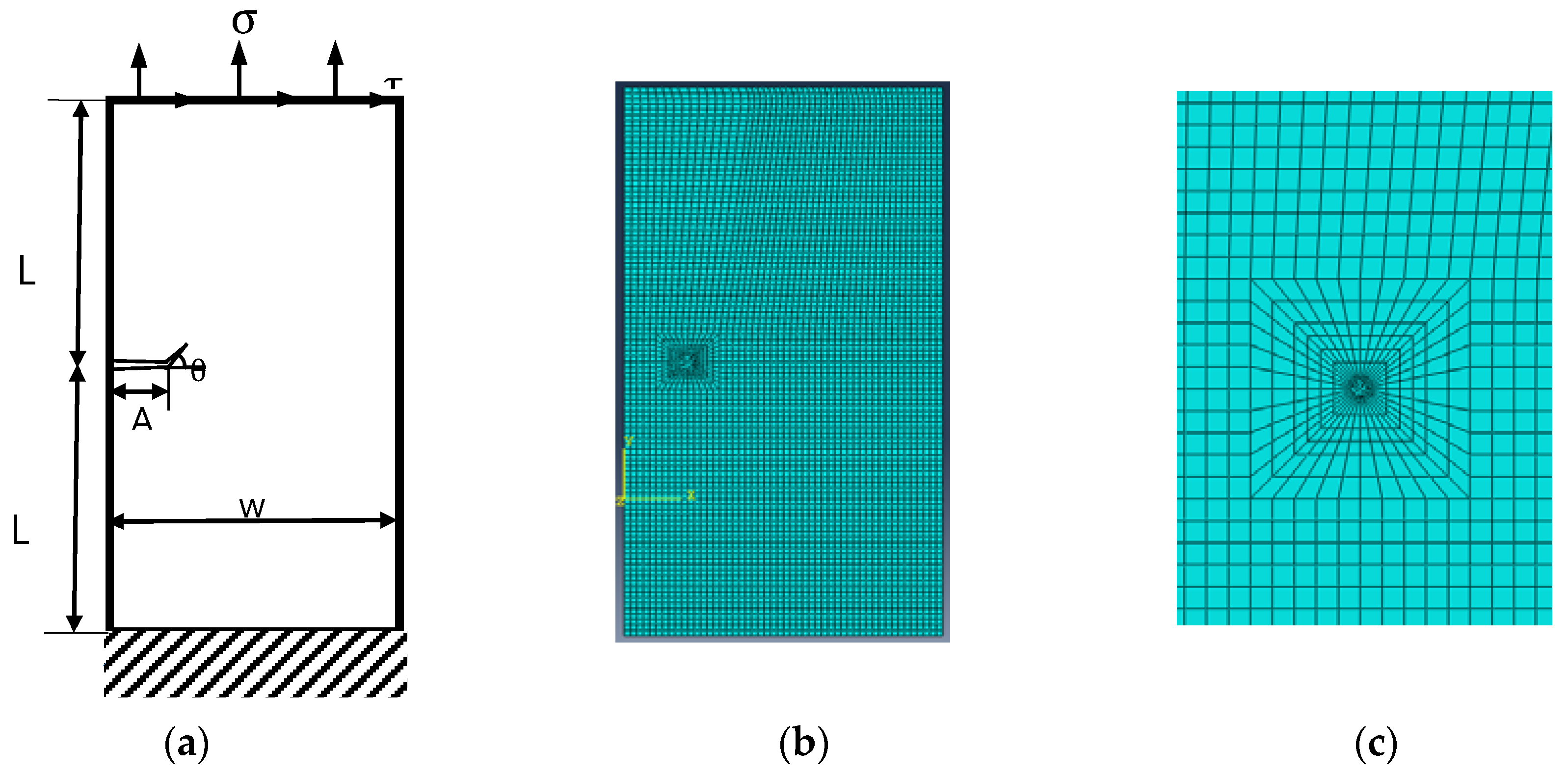
2.1. Numerical Analysis of 2D Crack
2.1.1. Crack Simulation with ABAQUS
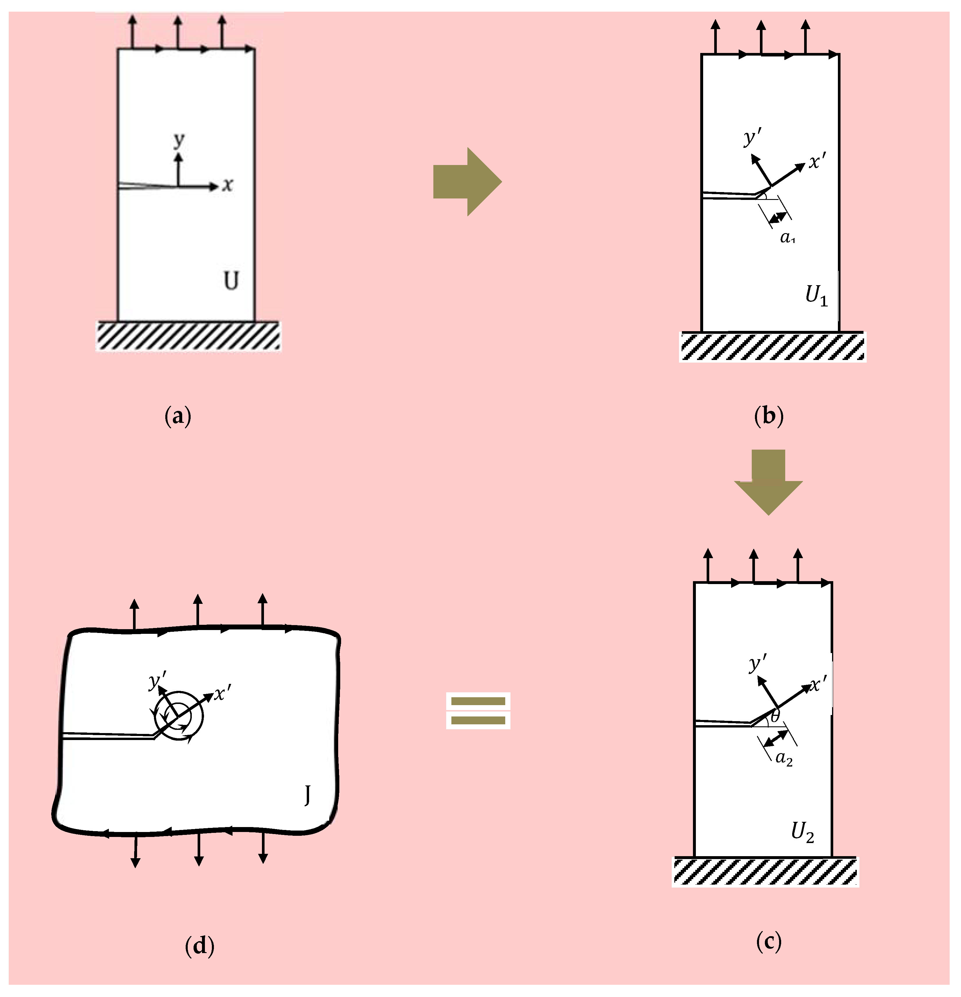
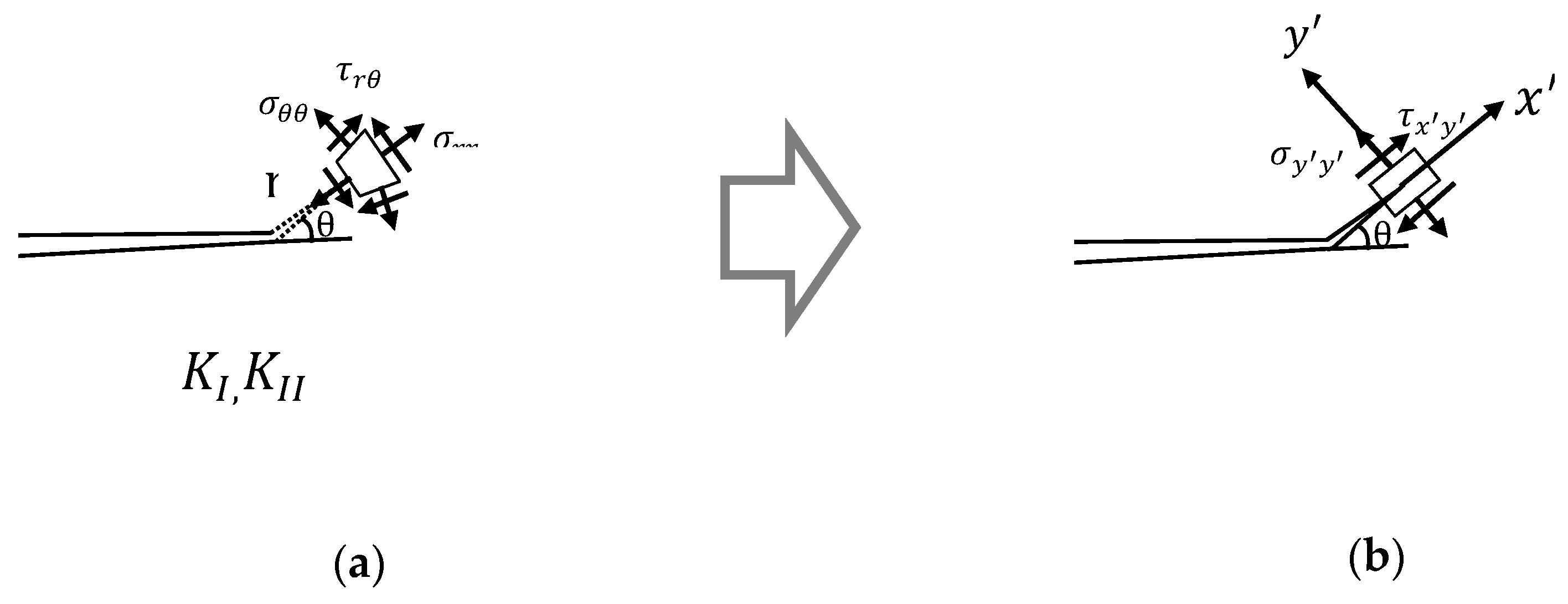
2.1.2. The Theoretical Basis of Energy Release Rate Definition
- (1)
- Obtain the values of and strain energy at the points
- (2)
- The energy differences between are calculated and divided by It represents the energy release rate for the crack at 0.05 mm, 0.15 mm, 0.25 mm, 0.5 mm.
- (3)
- Determine that the minimum value of kink length for calculation is 0.1 mm; since the kink crack becomes infinitesimally small, the values from the energy difference deviate from the integral.
2.1.3. Computational Analysis
- (1)
- Determine and under arbitrary combined Mode and Mode loading conditions with the initial crack.
- (2)
- Determine for kink cracks repeatedly, varying the kink length from to with four data points . Then, compute energy release rate as the kink propagation vanishes on the curve of versus kink length by the method of fitting.
- (3)
- Plot the non-dimensional value () for each kink angle ()
- (4)
- Determine the parameters of inclined ellipses that fit the above data points using the curve fitting algorithm by MATLAB, and the corresponding ellipse equation is presented as follows:where , , are the semi-major axis, semi-minor axis and inclination of ellipse, respectively.
- (5)
- Obtain the coefficients of quadratic of energy release rate in terms of stress intensity factors, and defined as
2.2. Discussion of Numerical Results
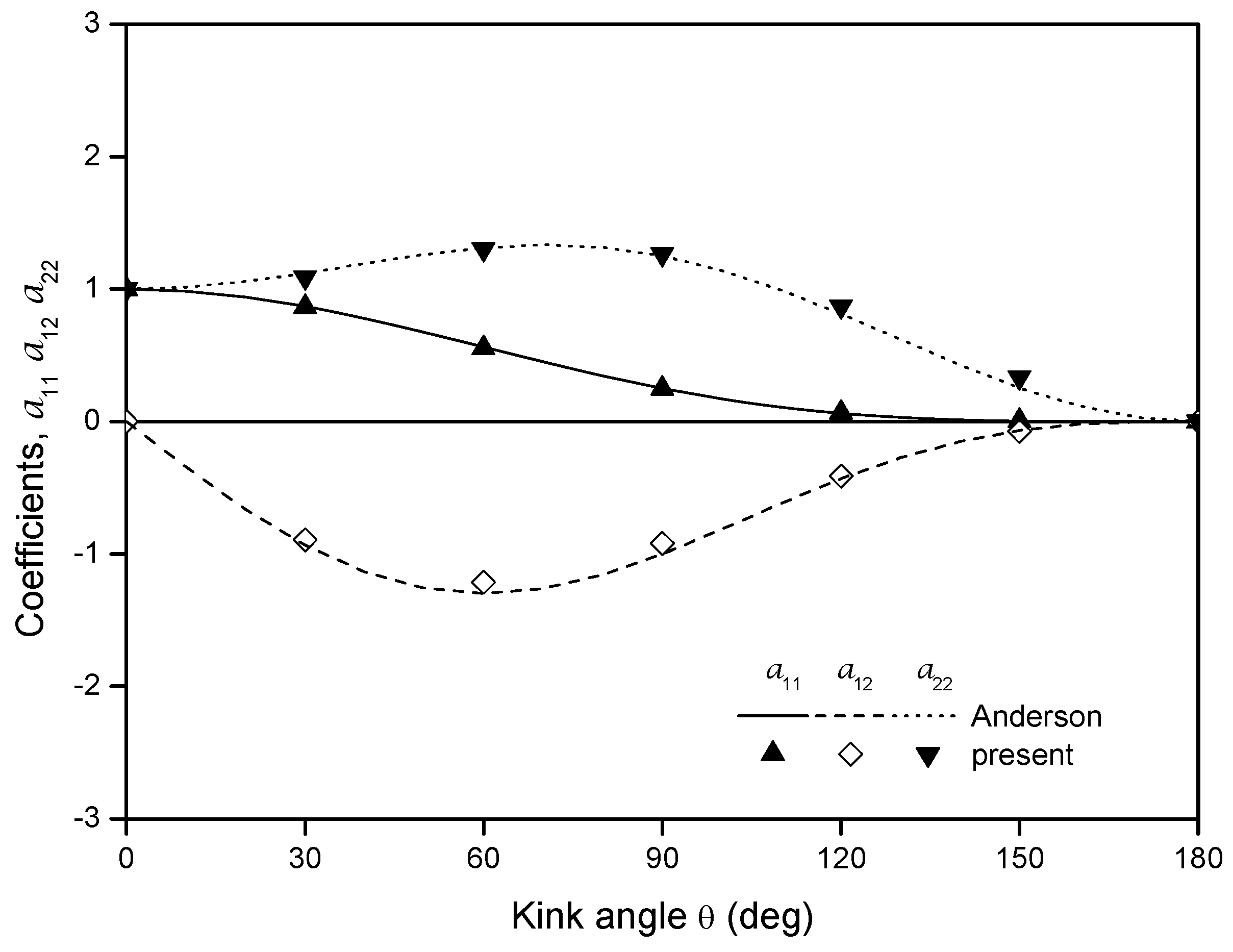
2.2.1. Comparison with References
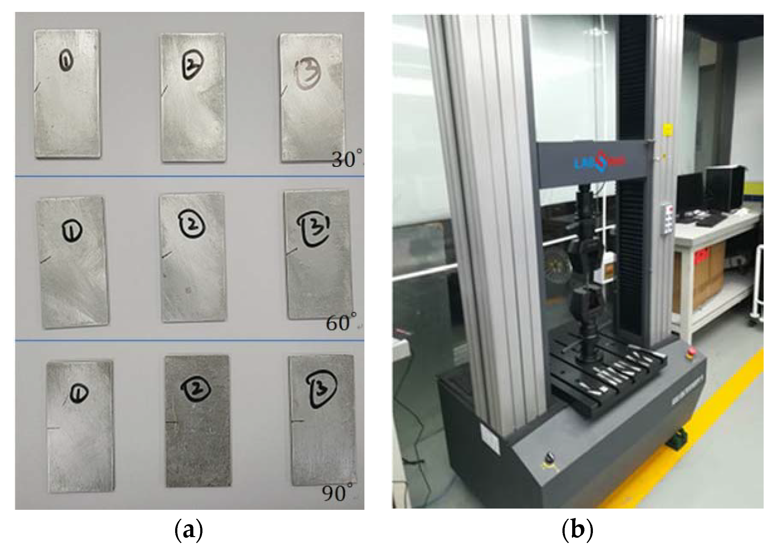
2.2.2. Experiment Verification
3. Fracture Parameters for 3D Crack
3.1. The Theoretical Derivation of Energy Release Rate for I-II-III Mixed Mode Crack
3.2. Numerical Analysis of 3D Crack
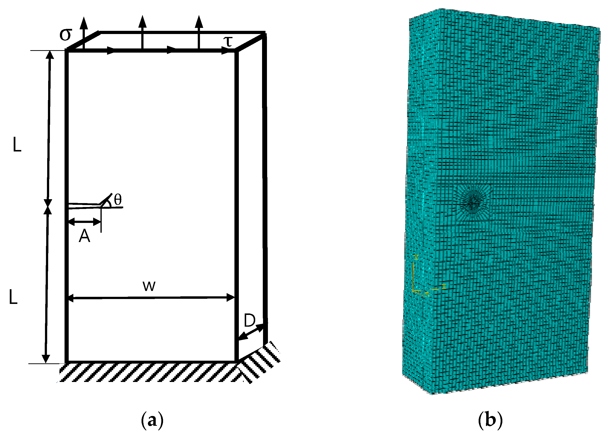
3.2.1. 3D Model of Crack Simulation
3.2.2. Computational Analysis
- (1)
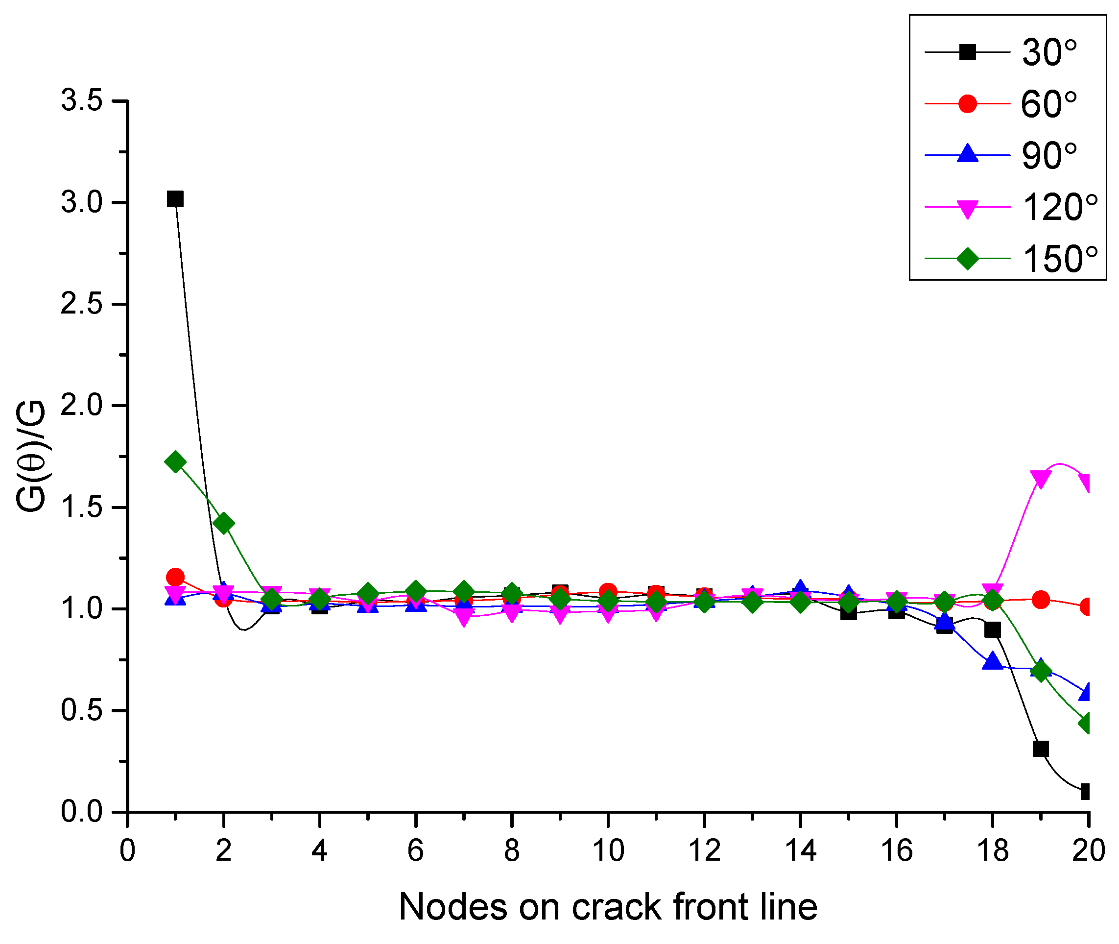
- Determine and for kink cracks repeatedly, varying the kink length from to with four data points . Then, compute the energy release rate as the kink propagation vanishes on the curve of and versus kink length through fitting each node on the crack tip line.
- (2)
- Plot the non-dimensional value () for each kink angle ()
- (3)
- Determine the parameters of inclined ellipses that fit the above data points using a fitting method for quadric surfaces in space by MATLAB, and the corresponding ellipse equation is presented as follows:where , , , are the semi-major axis, semi-middle axis, semi-minor axis and inclination of ellipse, respectively.
- (4)
- Obtain the coefficients of quadratic of energy release rate in terms of stress intensity factors, and defined as
- (1)
- The non-dimensional value ( ) transformed from the data output by ABAQUS forms a series of ellipsoids.
- (2)
- At each presupposed extended angle (30°~150°), the scattered points of dimensionless data output by ABAQUS under different loadings are all on the surface of the same tilted ellipsoid.
- (3)
- The coefficients of quadratics for energy release rate in terms of stress intensity factors are calculated for each kink angle based on the ellipsoid equations.
3.3. Discussion of Theoretical and Numerical Results
4. Conclusions
- (1)
- A relatively simple and precise numerical method was established to evaluate the energy release rate associated with the stress intensity factors under mixed mode loading based on the concept that the energy release rate is equal to the change rate of the energy difference before and after crack kinking.
- (2)
- Based on the numerical method, a series of spatial inclined ellipses in Mode I-II and ellipsoids in Mode I-II-III with different propagation angles computed from non-dimensional value () were fitted by MATLAB, and the expression of the energy release rate with the crack propagation angle was obtained.
- (3)
- A theoretical expression of energy release rate at any propagation angle for a crack tip under I-II-III mixed mode crack was deduced based on the propagation mechanism of the crack tip under the influence of a stress field. It is confirmed that the theoretical expression deduced could provide results as accurately as the present numerical method.
- (4)
- The present results are consistent with the experimental data. The error, which is lower than 5%, can be accepted considering that the specimens are not manufactured using ideal elastic material. Consequently, the present results demonstrate the simpler, accurate calculation process and the accurate evaluation of energy release rate.
Author Contributions
Funding
Conflicts of Interest
Nomenclature
| Energy release rate | |
| and | Stress intensity factor, and for Mode I, Mode II, Mode III. |
| Elastic modulus | |
| Poisson’s ratio | |
| Shear modulus | |
| Length of rectangular plate | |
| Wide of rectangular plate | |
| Thickness of rectangular plate | |
| Length of initial crack | |
| Kinking angel of crack | |
| Normal stress | |
| Shear stress | |
| Length of kink crack | |
| , | Strain energy before kink extension and after kink extension |
| Integral for a kink | |
| , , | Semi-major axis, semi-minor axis and inclination of ellipse |
| Oblique angle of crack | |
| Stress fields in polar coordinate | |
| Local stress intensity factors |
References
- Irwin, G.R. Onset of Fast Crack Propagation in High Strength Steel and Aluminum Alloys; Naval Research Lab: Washington, DC, USA, 1956; Sagamore Research Conference Proceedings; Volume 2, pp. 289–305. [Google Scholar]
- Chatterjee, S.N. The stress field in the neighborhood of a branched crack in an infinite elastic sheet. Int. J. Solids Struct. 1975, 11, 521–538. [Google Scholar] [CrossRef]
- Yukio, U.; Kazuo, I.; Tetsuya, Y.; Mitsuru, A. Characteristics of brittle fracture under general combined modes including those under bi-axial tensile loads. Eng. Fract. Mech. 1983, 18, 1131–1158. [Google Scholar] [CrossRef]
- Melin, S. Fracture from a straight crack subjected to mixed mode loading. Int. J. Fract. 1987, 32, 257–263. [Google Scholar]
- He, M.Y.; Bartlett, A.; Evans, A.G.; Hutchinson, J.W. Kinking of a crack out of an interface: Role of in-plane stress. J. Am. Ceram. Soc. 1991, 74, 767–771. [Google Scholar] [CrossRef]
- Kishen, J.M.C.; Singh, K.D. Stress intensity factors based fracture criteria for kinking and branching of interface crack: Application to dams. Eng. Fract. Mechan. 2001, 68, 201–219. [Google Scholar] [CrossRef]
- Hammouda, M.M.; Fayed, A.S.; Sallam, H.E. Simulation of mixed mode I/II cyclic deformation at the tip of a short kinked inclined crack with frictional surfaces. Int. J. Fatigue 2003, 25, 743–753. [Google Scholar] [CrossRef]
- Pantano, A. Cohesive model for the simulation of crack initiation and propagation in mixed-mode I/II in composite materials. Appl. Compos. Mater. 2019, 26, 1207–1225. [Google Scholar] [CrossRef]
- Li, X.F.; Lee, K.Y.; Tang, G.J. Kink angle and fracture load for an angled crack subjected to far-field compressive loading. Eng. Fract. Mech. 2012, 82, 172–184. [Google Scholar] [CrossRef]
- Fajdiga, G.; Zafošnik, B. Determining a kink angle of a crack in mixed mode fracture using maximum energy release rate, SED and MTS criteria. J. Multidiscip. Eng. Sci. Technol. 2015, 2, 356–362. [Google Scholar]
- Guo, B.K.; Yan, H.H.; Zhang, L. Cracking angle of an arbitrary oriented crack embedded in a strip under I-II mixed mode loading. Int. J. Mater. Sci. 2016, 6, 52–57. [Google Scholar] [CrossRef]
- Hussain, M.; Pu, S.; Underwood, J. Strain Energy Release Rate for a Crack under Combined Mode I and Mode II. In Fracture Analysis: Proceedings of the 1973 National Symposium on Fracture Mechanics, Part II; Irwin, G., Ed.; ASTM International: West Conshohocken, PA, USA, 1974; pp. 2–28. [Google Scholar]
- Wu, C.H. Fracture under Combined Loads by Maximum-Energy-Release-Rate Criterion. J. Appl. Mech. 1978, 45, 553–558. [Google Scholar] [CrossRef]
- Hayashi, K.; Nemat-Nasser, S. Energy-Release Rate and Crack Kinking Under Combined Loading. Trans. ASME 1981, 48, 520–524. [Google Scholar] [CrossRef]
- Chambolle, A.; Francfort, G.A.; Marigo, J.J. Revisiting energy release rates in brittle fracture. Nonlinear Sci. 2010, 20, 395–424. [Google Scholar] [CrossRef]
- Amestoy, M.; Leblond, J.B. Crack path in plane situations-II. Detailed form of the expansion of the stress intensity factors. Int. J. Solids Struct. 1992, 29, 465–501. [Google Scholar] [CrossRef]
- Azhdari, A.; Nemat-Nasser, S. Energy-Release Rate and Crack Kinking in Anisotropic Brittle Solids. J. Mech. Phys. Solids 1996, 44, 929–951. [Google Scholar] [CrossRef]
- Sih, G.C.; Paris, P.C.; Erdogan, F. Crack-Tip, Stress-Intensity Factors for Plane Extension and Plate Bending Problems. J. Appl. Mech. 1962, 29, 306–312. [Google Scholar] [CrossRef]
- Erdogan, F.; Sih, G.C. On the Crack Extension in Plates Under Plane Loading and Transverse Shear. J. Basic Eng. 1997, 12, 527. [Google Scholar] [CrossRef]
- Qizhi, W.; Xing, Z.; Qingzhi, H. Stress Intensity Factor; Springer Netherlands: Berlin, Germany, 2008. [Google Scholar]
- Anderson, T.L. Fracture Mechanics Fundamentals and Applications; CRC Press: Boca Raton, FL, USA, 2005. [Google Scholar]
- Richard, H.A. Specimens for Investigating Biaxial Fracture and Fatigue Process. In Biaxial and Multiaxial Fatigue; Brown, M.W., Miller, K.J., Eds.; Mechanical Engineering Publications: London, UK, 1989; pp. 217–229. [Google Scholar]
- Luca, S.; John, Y.; Alfredo, N.; Thierry, P.-L. Fracture and Structural Integrity: Annals 2014; Gruppo Italiano Frattura: Cassino, Italy, 2014. [Google Scholar]
- Pantano, A.; Averill, R.C. A Penalty-Based Interface Technology for Coupling Independently Modeled Three-Dimensional Finite Element Meshes. Finite Elem. Anal. Des. 2007, 43, 271–286. [Google Scholar] [CrossRef]


(deg) | kI(θ) from ABAQUS () | kII(θ) from ABAQUS | G(θ) for Calculation (mJ) | G for Simulation (mJ) |
| 30° | 1.31 × 10⁵ | 9.90 × 10⁵ | 4.84 | 4.84 |
| 60° | −5.01 × 10⁵ | 6.26 × 10⁵ | 3.12 | 3.17 |
| 90° | −7.72 × 10⁵ | 1.30 × 10⁵ | 2.98 | 2.98 |
| 120° | −6.88 × 10⁵ | −2.42 × 10⁵ | 2.58 | 2.58 |
| 150° | −4.02 × 10⁵ | −3.22 × 10⁵ | 1.29 | 1.29 |
| 180° | 0.00 × 100 | 0.00 × 100 | 0.00 | 0.00 |
(deg) | kI(θ) from ABAQUS | kII(θ) from ABAQUS | G for Calculation (mJ) | G for Simulation (mJ) |
| 30° | 2.91 × 10⁶ | 1.18 × 10⁶ | 47.82 | 47.82 |
| 60° | 1.85 × 10⁶ | 1.46 × 10⁶ | 26.84 | 26.84 |
| 90° | 8.14 × 10⁵ | 1.18 × 10⁶ | 10.02 | 10.01 |
| 120° | 1.50 × 10⁵ | 5.97 × 10⁵ | 1.84 | 1.84 |
| 150° | −8.86 × 10⁴ | 1.02 × 10⁵ | 0.09 | 0.09 |
| 180° | 0.00 × 100 | 0.00 × 100 | 0.00 | 0.00 |
| Chemical Composition | Cu | Si | Fe | Mn | Mg | Zn | Cr | Ti | other | AL |
|---|---|---|---|---|---|---|---|---|---|---|
| Ratio | 25% | 60% | 70% | 15% | 85% | 25% | 16% | 15% | 15% | margin |
| Crack Angle (°) | Sample Number | Calculated Extension Angle (°) | Experimental Extension Angle (°) | Experimental Extension Angle (Average) (°) | Error (°) |
|---|---|---|---|---|---|
| 30 | 1 | −60 | −59 | −58.70 | 2.17 |
| 2 | −60 | −59.5 | |||
| 3 | −60 | −57.6 | |||
| 60 | 1 | −43 | −41.5 | −41.17 | 4.26 |
| 2 | −43 | −40.8 | |||
| 3 | −43 | −41.2 | |||
| 90 | 1 | 0 | 0 | 0 | 0 |
| 2 | 0 | 0 | |||
| 3 | 0 | 0 |
© 2020 by the authors. Licensee MDPI, Basel, Switzerland. This article is an open access article distributed under the terms and conditions of the Creative Commons Attribution (CC BY) license (http://creativecommons.org/licenses/by/4.0/).
Share and Cite
Yang, Y.; Chu, S.J.; Huang, W.s.; Chen, H. Crack Growth and Energy Release Rate for an Angled Crack under Mixed Mode Loading. Appl. Sci. 2020, 10, 4227. https://doi.org/10.3390/app10124227
Yang Y, Chu SJ, Huang Ws, Chen H. Crack Growth and Energy Release Rate for an Angled Crack under Mixed Mode Loading. Applied Sciences. 2020; 10(12):4227. https://doi.org/10.3390/app10124227
Chicago/Turabian StyleYang, Yali, Seok Jae Chu, Wei song Huang, and Hao Chen. 2020. "Crack Growth and Energy Release Rate for an Angled Crack under Mixed Mode Loading" Applied Sciences 10, no. 12: 4227. https://doi.org/10.3390/app10124227
APA StyleYang, Y., Chu, S. J., Huang, W. s., & Chen, H. (2020). Crack Growth and Energy Release Rate for an Angled Crack under Mixed Mode Loading. Applied Sciences, 10(12), 4227. https://doi.org/10.3390/app10124227