Mid-Infrared Laser Spectroscopy Detection and Quantification of Explosives in Soils Using Multivariate Analysis and Artificial Intelligence

Abstract

A tunable quantum cascade laser (QCL) spectrometer was used to develop methods for detecting and quantifying high explosives (HE) in soil based on multivariate analysis (MVA) and artificial intelligence (AI). For quantification, mixes of 2,4-dinitrotoluene (DNT) of concentrations from 0% to 20% w/w with soil samples were investigated. Three types of soils, bentonite, synthetic soil, and natural soil, were used. A partial least squares (PLS) regression model was generated for predicting DNT concentrations. To increase the selectivity, the model was trained and evaluated using additional analytes as interferences, including other HEs such as pentaerythritol tetranitrate (PETN), trinitrotoluene (TNT), cyclotrimethylenetrinitramine (RDX), and non-explosives such as benzoic acid and ibuprofen. For the detection experiments, mixes of different explosives with soils were used to implement two AI strategies. In the first strategy, the spectra of the samples were compared with spectra of soils stored in a database to identify the most similar soils based on QCL spectroscopy. Next, a preprocessing based on classical least squares (Pre-CLS) was applied to the spectra of soils selected from the database. The parameter obtained based on the sum of the weights of Pre-CLS was used to generate a simple binary discrimination model for distinguishing between contaminated and uncontaminated soils, achieving an accuracy of 0.877. In the second AI strategy, the same parameter was added to a principal component matrix obtained from spectral data of samples and used to generate multi-classification models based on different machine learning algorithms. A random forest model worked best with 0.996 accuracy and allowing to distinguish between soils contaminated with DNT, TNT, or RDX and uncontaminated soils.

1. Introduction

The intensive use of high explosives (HEs) in military operations and mining excavations has contributed to soil contamination. Providing that HEs and their decomposition products that are highly persistent, mutagenic, and classified as Group C human carcinogens threaten human health [1,2], research on the timely detection of HEs has continued to receive considerable attention over the past few years. The methods currently used to detect HEs include gas chromatography-mass spectroscopy (GC-MS), gas chromatography-chemiluminescence (GC-CL), ion mobility spectrometry (IMS) [3], immunosensors [4], electrophoresis [5], fluorescence [6], high-pressure liquid chromatography (HPLC) [7,8], HPLC/mass spectrometry [7], and photo-assisted electrochemical detection [9]. However, none of these methods provides the required speed or accuracy for in situ detection of HEs in the presence of solid interfering materials.

Soil is considered to be a challenging matrix of organic compounds that interfere with HEs, making the detection of HEs in soils a difficult task [10,11,12]. While remote sensing has been applied to soils, the proposed system is complex [13]. Other studies conducted by the same research group involved the characterization [14,15,16], interaction [17,18,19], and detection [20,21] of HEs using Raman and Fourier-transform infrared (FT-IR) spectroscopy [22,23]. The detection of HEs was only marginally possible in all these cases providing that crystalline samples of explosives must be found within the solid matrix by microscopy to achieve the detection. The in situ detection of HEs in real soils with high selectivity and sensitivity has not been reported yet. In this study, a small, portable, and easy to handle system employing mid-infrared (MIR) quantum cascade laser (QCL) source [24] was used for analyzing HEs in soils at a distance of 15 cm. Furthermore, multivariate analysis (MVA) and artificial intelligence (AI) techniques were employed to quantify and detect the analytes of interest on the soil samples studied dosed with complex matrices of organic compounds [25].

External cavity QCLs provide ample wavelength tunability, justifying studies on threat chemicals [26,27,28,29,30] and biological compounds and microorganisms [31] with broad absorption features, including solids. QCLs were first demonstrated in 1994 [32]. These devices offer multiple benefits such as room-temperature operation, small sizes, long lifetimes, low energy consumption, long-term power stability, and fine-tuning of the output frequency [33]. Moreover, they provide an opportunity to devise portable systems for remote testing with excellent sensitivity, particularly on samples with low reflectivity or high absorptivity in the MIR range, such as soils. Compared to the existing sources in the MIR range, QCL sources have a higher output power that allows remote sensing and analysis. The rapid detection of HEs on highly reflective substrates using this method was demonstrated and reported by other investigators [34,35,36,37,38]. This spectroscopic analysis can be achieved without contact and in a non-destructive way. A study conducted at Pacific Northwest National Lab [39] demonstrated that the possibility of remote detection of many important HEs, including trinitrotoluene (TNT), cyclotrimethylenetrinitramine (RDX), and Tetryl, occurs in the spectral fingerprint window from 800 to 1400 cm⁻¹. This spectral window corresponds to the fingerprint region of the HE samples deposited on painted metal car doors. Other studies have demonstrated diverse QCL approaches to the rapid identification and characterization of HEs, given the routine requirements of security checks [40,41].

QCLs can provide significant benefits for public safety, particularly in locations such as airports, railways, bus stations, sports stadiums, and marathon sites. Therefore, this study is focused on the quantification and detection of HEs in soils [25] using a QCL source to enable remote sensing [42,43,44,45,46,47,48,49,50,51,52,53]. The limit of detection (LOD) was calculated for QCL spectroscopy based on the calibration curves of one HE in solid mixtures. The statistical figure of merit (FM) was achieved using the partial least squares (PLS) multivariate algorithm. Other FMs were also calculated.

Furthermore, AI methods were employed to achieve HE detection. In the future, two main applications can be developed based on the outcomes of this research. First, the proposed methods can be used to detect explosives on ordinary, non-ideal, low-reflective, real-world solid matrices. Second, the methods can be employed to detect HEs on natural solid matrices; for example, they can be used to locate landmines in sites affected by war and conflicts throughout the world, both for military purposes and implementing humanitarian demining applications.

2. Materials and Methods

2.1. Reagents

The HEs used as analytes in this study were 2,4-dinitrotoluene (2,4-DNT or DNT for simplicity), pentaerythritol tetranitrate (PETN), RDX, and 2,4,6-TNT (or TNT for simplicity). These materials were synthesized in a laboratory, except DNT and TNT, which were purchased from Chem Service (West Chester, PA, USA). Other studied analytes were potassium bromide (KBr), benzoic acid (BA), and ibuprofen (IBP), which were purchased from Sigma-Aldrich (Millipore Sigma, Merck KGaA, St. Louis, MO, USA). Bentonite clay (BC) was also obtained from Sigma-Aldrich. Synthetic soil samples (SYN-S) were prepared from washed sea sand and alundum™ cement, purchased from Thermo-Fisher Scientific (TFS) International, 75–300 mesh silica gel (TFS, Pittsburgh, PA, USA), as well as montmorillonite, bentonite, and activated charcoal purchased from Sigma-Aldrich (Milwaukee, WI, USA). A natural soil sample (NAT-S) was obtained from local sites located near the municipality of Mayagüez, PR, USA, with the coordinates 18°13′25.7″ N and 67°07′51.2″ W. Finally, another natural soil sample (NAT2-S) was obtained from the coordinates 18°9′36″ N, and 67°6′40″ W and used to evaluate the model.

2.2. Sample Preparation

Samples containing from 0% to 20% DNT w/w and a total mixture mass of approximately 0.20 g were prepared for the quantification analysis. The initial set of 10 samples and replicates entailed mixtures of several matrices with DNT. The matrices consisted of KBr, BC, SYN-S, and NAT-S. The SYN-S comprised 37% bentonite, 27% alundum™ cement, 16% montmorillonite, 10% silica gel, 8% washed sea sand, and 2% activated charcoal. The samples were prepared by grinding the HE into a fine powder using a mortar and pestle, followed by mixing in a mini vortex mixer for approximately 10 s at 3000 rpm. The mixed samples were ground again and mixed in the mini vortex mixer for a second time. Mixtures of KBr and NAT-S with lower concentrations of DNT, approximately from 0% to 3% by weight, were made and named KBr Low and NAT-S Low, respectively. Only these matrices were prepared and tested for comparing the variation of the results with the change of the concentration range. The preparation of these samples was similar to that of the others, except for using different DNT concentrations.

Mixtures containing other highly intrusive compounds such as explosives (TNT, RDX, and PETN) and non-explosives (BA and IBP) were prepared using the same preparation method with only one concentration per interference analytes, namely, 10% w/w. These samples were tested using the PLS model of DNT mixed with NAT-S. For the pattern recognition analysis based on AI, samples of mixtures containing from 0% to 20% of DNT, TNT, and RDX by weight in three soil types (BC and two NAT-S samples) were prepared.

2.3. Soil Characterization

Soil samples from Mayagüez, PR (USA) were characterized using thermogravimetric analysis (TGA) to measure the water content, sand and clay percentages, and total organic matter (TOM) [54]. TOM values were determined by oxidation with hydrogen peroxide [55,56] and calcination [55]. The total dissolved solids levels were measured by dissolving soil in water, followed by its filtering and drying. The percent distributions of components in the Mayagüez-PR NAT-S samples are illustrated in the Supplementary Materials: Table S1.

2.4. Data Acquisition and QCL System

The background spectrum of a KBr substrate was obtained before measuring the QCL spectra of the samples. Providing the lack of MIR signals from the employed solid matrix, this background spectrum provided an excellent and smooth reference trace. The first samples were then placed in the wells of metal holders (1.1 cm in diameter and 3 mm deep). Duplicate spectra were collected at 10 different locations on the sample surfaces, resulting in a total of 20 spectra per sample. Sixteen ranges were used for calibration and internal validation or cross-validation (CV), while the remaining four spectra were used for testing or external validation. This process was repeated for each concentration. The spectra were obtained in the reflectance mode at a distance of approximately 15 cm using a LaserScan™ MIR pre-dispersive spectrometer (Block Engineering, Marlborough, MA, USA) equipped with three tunable MIR lasers diodes having a tuning range from 990 to 1111 cm⁻¹, 1111 to 1178 cm⁻¹, and 1178 to 1600 cm⁻¹ The spectral linewidth was < 2 cm⁻¹ and the scan time was approximately 1.5 s for each of the diodes. The average power typically varied between 0.5 and 10 mW across the entire tuning range of ≈ 600 cm⁻¹ with 100:1 Transverse Electromagnetic Mode (TEM₀₀) polarization and a beam divergence of < 2.5 mrad in the x-axis and < 5 mrad in the y-axis. The spectrometer had a 7.6-cm diameter ZnSe lens, which was used to focus the MIR beam to collect the reflected light and focus the light onto a thermoelectrically cooled mercury–cadmium–telluride (MCT) detector. The wavelength accuracy and precision were 0.5 and 0.2 cm⁻¹, respectively. The spectroscopic system worked best at a distance to the target of 15 ± 3 cm, with each laser producing an elliptical spot with diameters of 4 and 2 mm in the same space at a distance of 15 cm due to the difference of beam divergence in the axes (Galan-Freyle et al. [30]).

2.5. Data Quantification Analysis

The OPUS™ data acquisition and analysis software (v. 4.2 and v. 6.0, Bruker Optics, Billerica, MA, USA) were used to perform the multivariate data analysis. Calibration curves were generated from the PLS models of DNT in the studied solid mixtures, and the uncertainties and FM for this model were estimated. The accuracies of the multivariate calibration curves were evaluated using the root-mean-square error of estimation (RMSEE), the root-mean-square error of CV (RMSECV), and root-mean-square error of prediction (RMSEP) for external validation. These parameters were used as criteria for evaluating the quality of the proposed method.

The linearity of the calibration curves was evaluated using the values of the coefficient of determination (R²), which indicates the percentage of variance present in the true component values reproduced by the PLS regression model. In contrast, the sensitivity (SEN) of multivariate methods can be estimated as the net analyte signal (NAS) [57] at a unit concentration as follows [58]:

SEN = 1/‖b‖,

(1)

where b denotes the regression vector of the PLS model. The analytical sensitivity (γ) can be defined similarly to univariate calibrations [59] as

γ = SEN/ε,

(2)

where ε denotes instrumental noise. In the absence of interferences, the NAS would be equal to the intensity of the total analyte signal. The noise level was measured by collecting 20 spectra of a blank (KBr) and calculating the average of the standard deviations for all wavenumbers.

The LOD was estimated using Equation (3) [60,61]:

LOD = Δ(α,β)*(RMSEE (1 + h_o)^1/2,

(3)

where h_o denotes the distance of the predicted sample to the mean of the calibration set at zero concentration and Δ(α,β) is a statistical parameter correlated with the α and β probabilities of falsely stating the presence or absence of the analyte. Δ(α,β) = 3.3 was used to compute the LOD values providing that the value for the degrees of freedom was > 25.

The residual prediction deviation or relative predictive determinant (RPD) was used to represent how the calibration model predicts a specific set. This value can also be used to evaluate the performance of a model in absolute terms. The RPD values can be calculated as

RPD = SD/SEP,

(4)

SEP = ((∑(Diff − Bias)²)/(N − 1))^1/2,

(5)

Bias = (∑Diff)/N,

(6)

where SD denotes the standard deviation, SEP is the standard error of prediction, N stands for the number of samples, and Diff indicates the difference in concentration values of the analytes between the predicted and reference sets.

2.6. Pattern Recognition Analysis

An algorithm for comparing different machine learning (ML) methods for classification was developed in Python 3 using the sklearn 3.2 library [62]. Ten ML methods for classification were employed: K-neighbors classifier, support vector machine for classification (SVM), decision tree classifier, random forest classifier (RFC), AdaBoost classifier (ABC), gradient boosting classifier, linear discriminant analysis, and quadratic discriminant analysis. A basic description of each ML method used in this study is included in Supplementary Materials: Table S2. Each classifier was trained using 53% of data, while the remaining 47% of data were reserved for testing. The method achieving the highest accuracy value and lowest log-loss value on the test data was considered to be the most efficient.

2.7. Artificial Intelligence Scheme

The spectra were preprocessed before they were evaluated by the ML methods. The preprocessing scheme employed in this study is shown in Figure 1. First, all spectra were normalized using vector normalization (VN) preprocessing. Next, the spectral data were reduced using principal component analysis (PCA) from 3057 points to 20 PCs. Separately, the preprocessed spectra were compared with those in a database of soils. Subsequently, a classical least squares preprocessing (Pre-CLS) [36] was applied to the original spectra to extract a parameter that was proportional to the percentage of soil from the database spectra. Finally, PCA and the extracted parameter were used to generate the ML models.

Pre-CLS is based on a linear model of classical least squares represented as

$$f\left({\phi }_j,{\beta }_j,{\omega }_i\right)={\beta }_0+{\beta }_1\phi {\left({\omega }_i\right)}_1+\cdots +{\beta }_j\phi {\left({\omega }_i\right)}_j,$$

(7)

where $f\left({\phi }_j,{\beta }_j,{\omega }_i\right)$ denotes the normalized calculated spectrum (CS) of soil derived from a mixture of several normalized spectra of soils $\phi {\left({\omega }_i\right)}_j$ recorded in the database of soils spectra (DBS); ${\omega }_i$ denotes the wavenumber and ${\beta }_j$ is a parameter indicating the fraction or proportion of $\phi {\left({\omega }_i\right)}_j$ of a particular component in the CS. The model assumes that there are no binding interactions among the components in the mixture, which implies that the intensity contributions are additive. The ${\beta }_j$ parameters can be calculated by finding the minimum of the square difference of the normalized intensity between the real spectrum and the CS. The minimum value of the sum of the squares of $d_i$(E) with respect to ${\beta }_j$ can be found by equating the first-order partial derivatives with respect to ${\beta }_j$ to zero and finding the ${\beta }_j$ values. Since the model contains n parameters, n partial derivative equations are generated as follows:

$$\frac{\partial d^2}{\partial {\beta }_j}=-2{\displaystyle \sum }_i{d}_i\frac{\partial f\left({\phi }_j,{\beta }_j,{\omega }_i\right)}{\partial {\beta }_j}=0,j=1,2,\cdots ,n$$

(8)

The value of $\phi {\left({\omega }_i\right)}_j$ can be determined using a simple forward selection algorithm (FSA). According to this algorithm, an empty model is generated first, and then variables (soils spectra from the database) are added one by one. At each next step, the E value shows the improvement of the model. The process is stopped when E cannot be further improved.

The criteria used to evaluate the performance of the classification models were recall, log-loss, precision, f1-score, weighted average, support, and accuracy. For binary classification, the recall of the positive class is also known as sensitivity, while the recall of the negative class is called specificity.

The log-loss function is used in (multinomial) logistic regression and its extensions, such as neural networks. It is defined as the negative log-likelihood of the true labels given the predictions of a probabilistic classifier. The log-loss is defined only for two or more labels. For a single sample with the true label yt and estimated probability yp that yt = 1, the log-loss is

−log P(yt|yp) = −(yt log(yp) + (1 − yt) log(1 − yp))

(9)

Precision is often called the positive predicted value and calculated as the ratio TP/(TP + FP), where TP denotes the number of true positives. FP denotes the number of false positives. Intuitively, precision is the ability of a classifier to not label a negative sample as positive. The f1-score is also known as the balanced f-score or the f-measure. The f1-score can be defined as a weighted average of precision and recall, where the f1-score best value is 1, and the worst is 0. The relative contributions of precision and recall to the f1-score are equal. The f1-score in the multi-class and multi-label cases is the average of the f1-score for each class with weighting that depends on the average between precision and recall. The f1-score can be calculated as

f1-score = 2 *(precision * recall)/(precision + recall)

(10)

The support is the number of used records, i.e., the number of spectra for each class. The classification accuracy score in multi-label classification computes the accuracy subset: the set of labels predicted for a sample should exactly match the corresponding set of actual labels in an ideal case.

3. Results and Discussion

3.1. Quantification Analysis

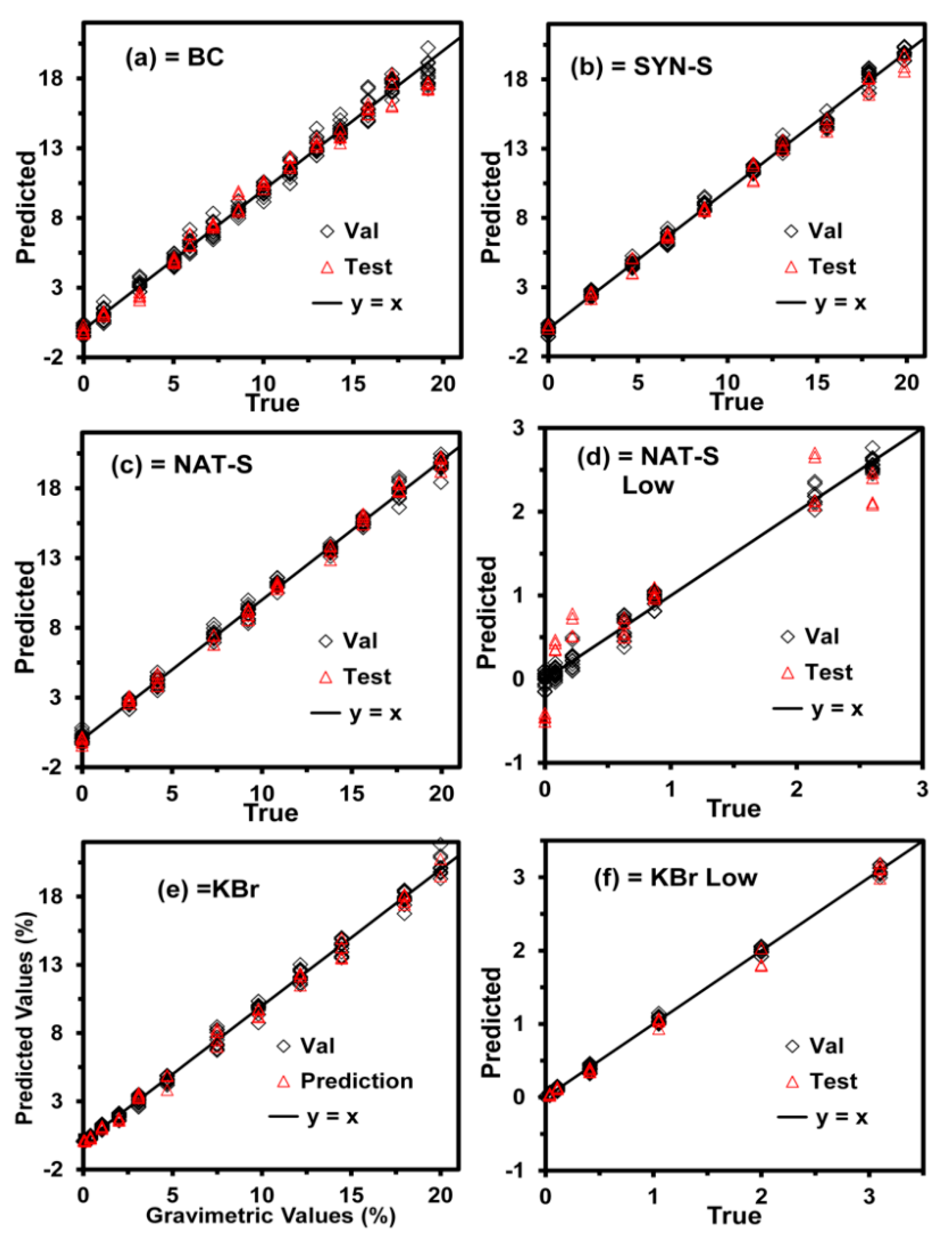
All spectra were converted to the Kubelka–Munk function [63] because the reflectance values for all samples were very low. This transformation is appropriate for the diffuse reflectance spectra of powders [64] with R values <60% [65]. The models were generated using this transformation. The graphs plotting the predicted versus true values for the samples used in CV and testing are shown in Figure 2, where the CV data are represented with open diamonds. In contrast, the test data are represented with open triangles. The solid black line represents the ideal case or perfect model (y = x), where the predicted values are equal to the true values throughout the entire data range.

The data set employed in CV was generated using the leave-one-out CV (LOO-CV). It can be noticed from Figure 2 that the predicted values for the CV and test data sets closely follow the best performance line (y = x). This alignment can also be confirmed by the low values of the RMSEE, RMSECV, and RMSEP listed in

Table 1. Accuracy, bias, and the number of latent variables (LV) for the studied models and matrices.

	RMSEE	RMSECV	RMSEP	Bias	LV
BC	0.41	0.57	0.70	−0.0007	11
SYN-S	0.35	0.43	0.53	−0.0069	7
NAT-S	0.25	0.39	0.39	0.0010	10
NAT-S Low	0.08	0.10	0.34	0.0100	7
KBr	0.18	0.32	0.41	−0.0044	10
KBr Low	0.02	0.03	0.08	−0.0003	9

.

All models were generated using the complete spectral window (1000–1600 cm⁻¹). In this study, VN was used as a preprocessing step as it proved to be better than the other tested preprocessing steps except for KBr. Other preprocessing steps were tested, such as mean centering (MC), linear offset subtraction, straight-line subtraction, minimum and maximum normalization, multiplicative scatter correction, first derivative, second derivative, and no preprocessing step. When applying VN, the average intensity is calculated first, and then this value is subtracted from the spectrum. Next, the sum of the squared intensities is calculated, and the spectrum is divided by the square root of this sum. Models for DNT in KBr were generated to evaluate the detection in the absence of interferences: one at high concentrations (0–20%) and another at low concentrations (0–3%). The errors for these models are listed in Table 1. The most effective preprocessing method for the KBr models was MC. This result suggests that VN is a suitable preprocessing step only when interferences from the matrix are present. In a model free from the interfering matrix (KBr), applying VN for generating samples with low concentrations had the same signal intensity as samples with high concentrations. This is reflected in the lousy prediction and high uncertainty for samples with low concentrations (see Supplementary Materials: Figure S3).

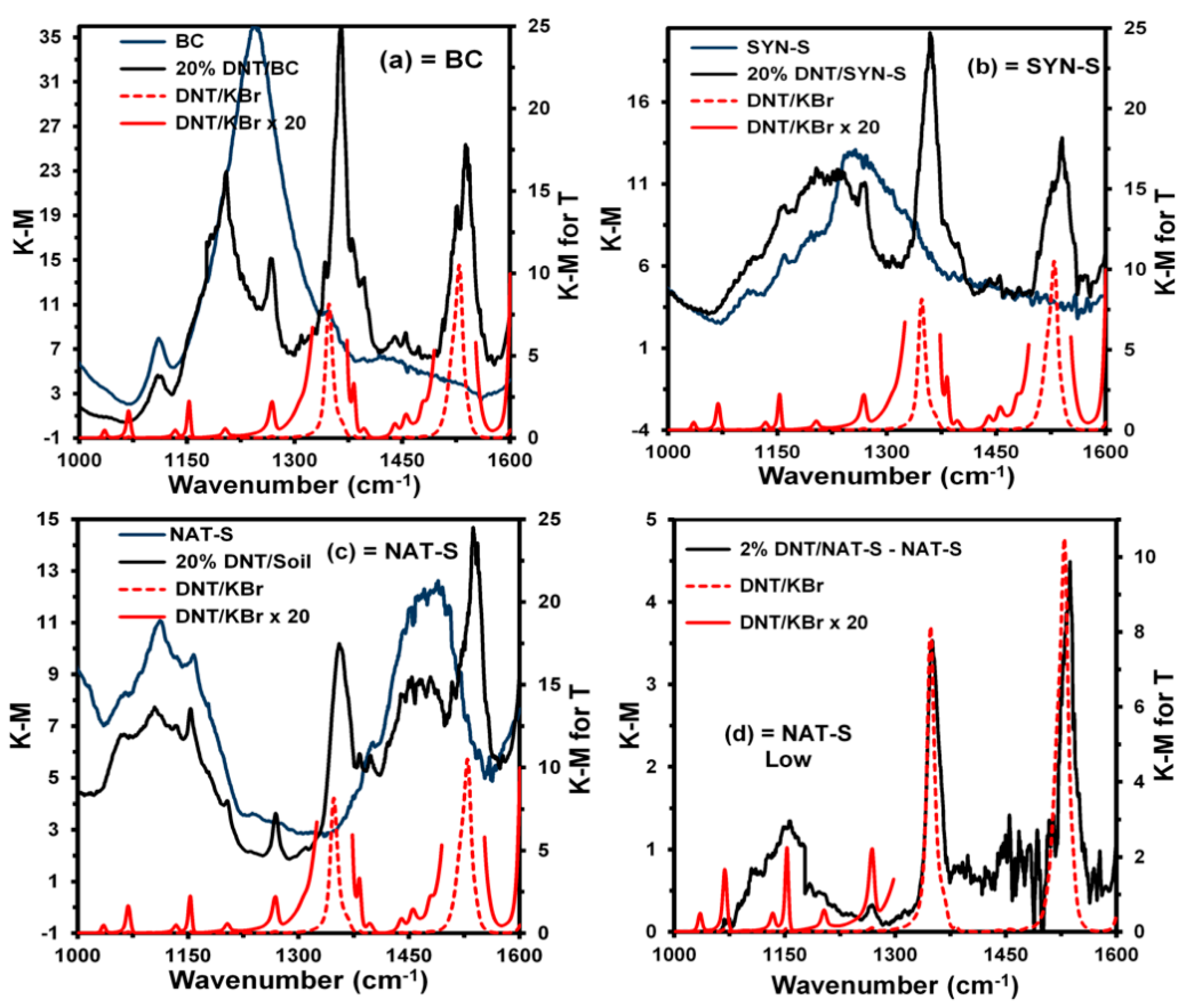
The spectra of the neat matrices, matrices with 20% DNT, and the corresponding standard reference spectra of DNT in KBr for transmittance are shown in Figure 3a–c, respectively. Figure 3d shows the resulting spectrum for the matrix with 2% DNT in NAT-S minus the spectrum of the neat matrix and corresponding standard reference spectra of DNT in KBr for transmittance. For clarity, DNT reference spectra are represented with the red, dotted lines. From these graphs, it is evident that DNT signals are observed on the background matrix signals in all cases, including 2% DNT in NAT-S.

Figures of Merit (FM)

The accuracies of the models were determined from the values of the RMSEE, RMSECV, and RMSEP. The results for each model (labeled by matrix) are listed in Table 1. The precision was inferred through the values of the relative standard deviation (RSD). The RSD values for the prediction of the same sample in the same site were calculated for different concentrations and their average to measure the repeatability (RSDr). The RSD values for the prediction of the same sample in various locations on the sample surfaces were calculated for different concentrations and their average to measure the mixture homogeneities (RSDh). The RSD values for different samples at the same concentration were calculated for different concentrations and their average to measure the reproducibility (RSDrd). From these values, which are listed in

Table 2. Relative standard deviation (RSD) and relative predictive determinant (RPD) values for the models generated.

	RSDr	RSDh	RSDrd	RPD-CV	RPD-Test
BC	2.4	5.5	12.7	9.7	11.3
SYN-S	1.5	5.3	9.1	9.2	16.2
NAT-S	2.2	4.2	4.8	16.1	27.6
NAT-S Low	3.2	13.8	32.9	9.1	12.6
KBr	3.4	3.6	4.1	19.8	36.5
KBr Low	5.7	6.2	11.9	27.5	50.1

, it can be concluded that the technique has excellent repeatability, while the samples have excellent homogeneity. However, only good reproducibility was determined for the models.

Another FM used for measuring precision was the RPD. As previously mentioned, the RPD is the ratio of the variation in the validation samples and the size of probable errors occurring during predictions. The RPD values are also listed in Table 2.

The best models were the ones with the lowest RMSEP values and the highest RPD values. The values obtained for the RPD were excellent. It has been suggested that models with RPD values greater than 5 can be considered suitable for quality control. On the other hand, models with RPD values greater than 6.5 can be used for process monitoring. Moreover, models with RPD values greater than 8 can be used in any application [66]. All the models tested in this study had RPD values higher than 8. This result indicates that the proposed technique can be used for the direct analysis of HE in soils. At the same time, the detection of explosives and their respective effects over different soil types have not been studied in detail so far. We plan to expand the present study to include reliable models over various types of soils as part of our future work.

In the context of determining HEs, sensitivity refers to the ability of a method or instrument to detect an analyte at a specified concentration. In contrast, the sensitivity of an analytical approach as defined in this study, is the capability of the method to discriminate between small differences in concentrations or masses of a target analyte. The sensitivity of each method studied was calculated according to Equations (1) and (2), and the results of these calculations are presented in

Table 3. Sensitivity, analytical sensitivity, the limit of detection (LOD), and noise of the models, with and without vector normalization (VN) preprocessing.

	VN
	LOD	SEN	γ	γ−1
BC	1.4	0.013	43	0.023
SYN-S	1.2	0.016	53	0.019
NAT-S	0.8	0.010	32	0.031
NAT-S Low	0.3	0.087	289	0.003
Noise = 0.0003
	No Preprocessing
	LOD	SEN	γ	γ−1
BC	2.3	1.48	39	0.025
SYN-S	1.4	2.25	60	0.017
NAT-S	1.0	1.36	36	0.028
NAT-S Low	0.6	20.63	552	0.002
KBr	0.6	0.51	14	0.072
KBr Low	0.07	1.26	34	0.029
Noise = 0.037

. The SEN value calculated for a model with VN preprocessing should be interpreted differently from the one without preprocessing or employing other preprocessing steps. Thus, the sensitivity values were derived from two types of models: models with VN as the preprocessing step and models without preprocessing steps. When using VN preprocessing, the spectra were normalized such that the sum of squares of intensity is equal to one. In other words, the spectra are converted to unit vectors. The SEN parameters were calculated from the magnitude of the vector calibration functions b, which, in turn, were derived from the spectra and their respective concentrations of standards. VN directly affects the magnitude ‖b‖ and value of SEN as a consequence. However, a better parameter for sensitivity can be obtained by calculating γ because this parameter is only affected by instrumental noises. The noise level was measured by collecting 20 spectra of a blank (target) and calculating an average of the standard deviations for all wavenumbers. The resulting noise for the models was different when considering 20 normalized spectra with VN (see Table 3). Otherwise, the γ-values calculated from the two types of models were very similar, which is an indication that γ is not affected by VN preprocessing or any other types of preprocessing.

The inverse of γ (denoted as γ⁻¹) provides an estimation of the minimum concentration difference (resultant) discernible by the model considering the instrumental noise as the only source of error. In the case of NAT-S Low, γ was 0.003% for the model with VN preprocessing and 0.002% for the model without preprocessing, with the difference being statistically insignificant. It is not possible to make a comparison of the sensitivities between the modes with matrix and without matrix because the magnitude of ‖b‖ depends on the number of signals and number of latent variables (LV) (see Supplementary Materials: Figure S5). For the models of spectra with many signals (BC, SYN-S, and NAT-S), the magnitude of ‖b‖ is higher than that for the models with low-intensity signals (KBr models). A better FM for this comparison is the LOD. For the models with the matrix (BC, SYN-S, and NAT-S), the LOD values are close to that of the model without the matrix (KBr models). Curves for the samples of low concentrations of DNT in NAT-S were generated to determine whether the employed concentration range influenced the LOD values of the curves. In these cases, the LOD decreased from 0.8% to 0.3%. DNT concentrations between 0.3% and 0.8% in the NAT-S Low model can be quantified with higher uncertainties and higher probabilities of false positives and missed detections because RSD should be between 10% and 33%.

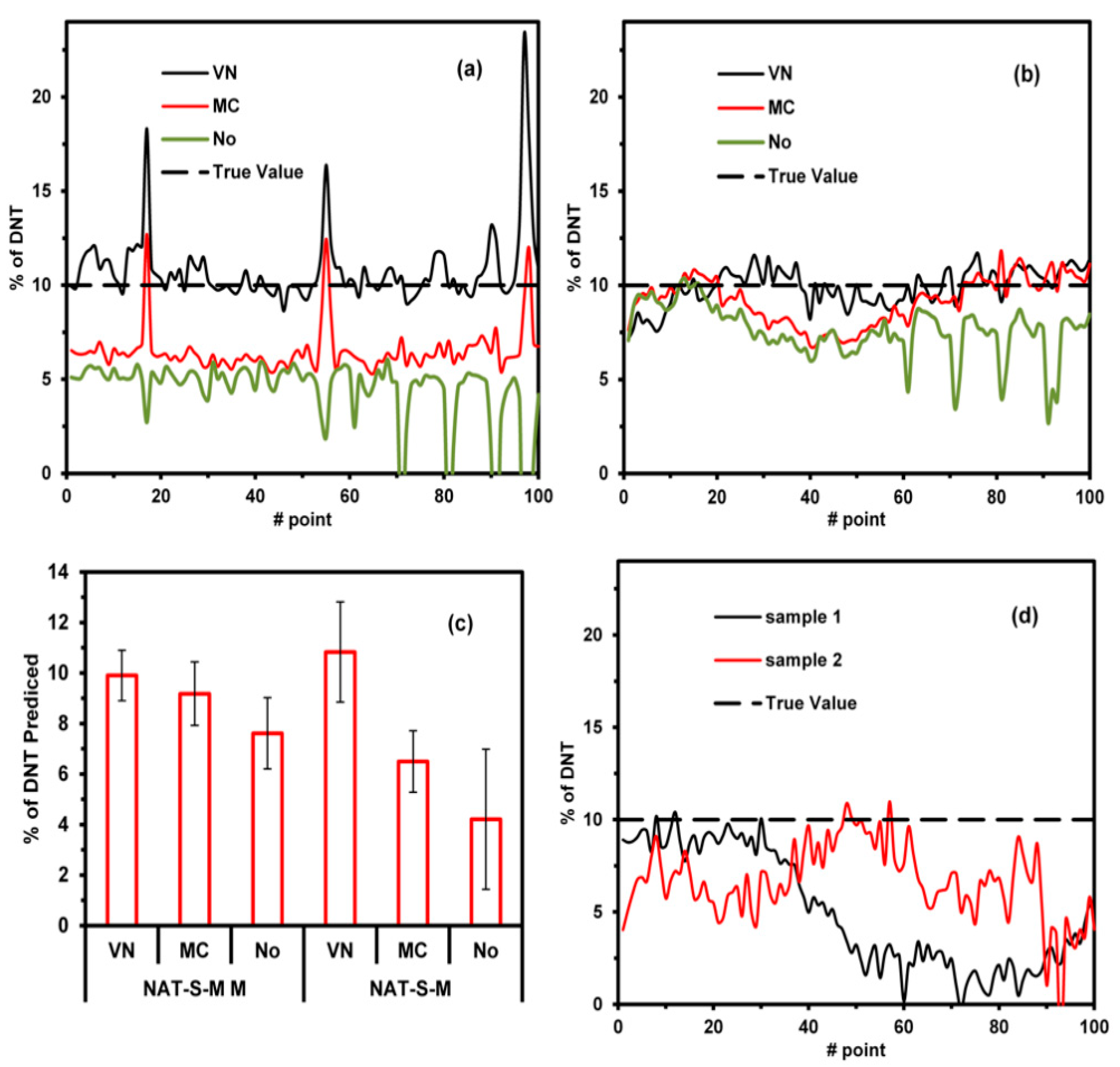
To test the NAT-S model, a map of three new types of samples was analyzed, and a map of 10 × 10 mm² (100 points) for each sample was generated. Two samples comprised the same soil as that used in the NAT-S models and were contaminated with 10% of DNT. The first sample consisted of a simple mixture (NAT-S-M). The second sample involved mixing and macerating the components (NAT-S-MM). The concentrations were predicted using the NAT-S model with three preprocessing methods: VN, MC, and no preprocessing. The map for the NAT-S model with VN is included in Supplementary Materials: Figures S6–S9, while the predictions for the 100 points for each map using different preprocessing methods are shown in Figure 4a,b. VN preprocessing applied to both samples (NAT-S-M and NAT-S-MM) resulted in better results, with the predicted values being close to the true value on average (10% DNT, see Figure 4c). MC preprocessing worked better in NAT-S-MM than NAT-S-M. This indicates that while the macerated process homogenized the size of the particles, MC was not able to compensate for the difference in the particle size. In contrast, the VN preprocessing method was able to compensate for these differences. The prediction of DNT in NAT-S-M shows peaks of high DNT concentrations (>10% DNT). This is because the particles of DNT were not homogenized. The models with no preprocessing provided bad predictions due to the difference in the baseline of the spectra. The above discussion demonstrates that VN preprocessing corrects the spectral variation due to changes in the particle size. To demonstrate the change in spectrum with the particle size, the tested soil was sieving for three particle sizes (d): d > 0.85 mm, 0.85 mm > d > 0.25 mm, and d < 0.25 mm. One hundred spectra were acquired at various locations on the sample surface for each value of d, and the average and standard deviation of the spectra were determined (see Supplementary Materials: Figures S10 and S11). The background offset spectral decreases with d, whereas the standard deviation increases with d; however, this pattern is not consistent throughout the spectra. It is higher in the 1000–1200-cm⁻¹ and 1400–1600-cm⁻¹ regions. This can be explained by the fact that MC is not able to correct the background offset spectral completely in contrast to VN; VN is better because it scales the spectrum to unit vectors, whereas MC only changes the baseline.

In the third sample, another type of natural soil (NAT2-S) was used to evaluate the NAT-S model. Two samples of NAT2-S were contaminated with 10% of DNT and mixed. Mappings of 10 × 10 mm² (100 points) were generated with the %DNT predicted from the NAT-S model using VN preprocessing. The mappings are present in Supplementary Materials: Figure S12, while predictions for each point are illustrated in Figure 4d. It can be noticed from the figure that the predictions were lower than the true values. This indicates that the NAT-S model quantifies below the true value of 10% DNT; however, it is capable of predicting the existence of an explosive in a soil. This indicates that the technique should be used in known soil to have good quantification.

To challenge the NAT-S model with other interferences, mixtures of other analytes in soil were prepared with a concentration of 10% (median of the model). The analytes used as interferences were BA, IBP, PETN, RDX, and TNT. BA and IBP do not have nitro groups but have aromatic rings and thus many common signals with DNT in the range of 1000–1600 cm⁻¹. PETN and RDX are nitro aliphatic explosives. TNT is very similar to DNT but considered to be a more challenging interference. Predictions for these samples were generated using the calibration curves for DNT/NAT-S. While the predicted values should have been zero or close to zero because the samples did not contain DNT, the average predicted concentrations were 8.8% (BA), 3.1% (IBP), -8.0% (PETN), 2.3% (RDX), and 25.8% (TNT) (see

Table 4. Prediction of %DNT from the NAT-S models.

	NAT-S	NAT-S OPT-Val
BA	8.8	0.02
IBP	3.8	−0.02
PENT	−8.0	0.00
RDX	2.3	0.02
TNT	25.8	0.11

). The objective was to measure the model’s capability of discriminating against these interferences.

To improve the model with respect to the recognition of interferences, an optimization procedure was applied. This procedure involved implementing the optimization of the most significant regions of the spectra after using various preprocessing steps. During optimization, the spectral region was divided into equal spectral sub-regions. Then, the optimum combination of sub-regions was determined by starting with 10 sub-regions and successively excluding one sub-region. This procedure continued until the values of the cross-validation errors did not improve further. The RMSECV values were calculated for each combination of the preprocessing steps, and the models with the lowest values of errors were selected. Twenty spectra of each interference were introduced together with the validation spectra set off with 0% of DNT true value. Then, optimization was performed by minimizing the RMSECV value. This was labeled as an optimization of the validation set (OPT-Val).

In OPT-Val, all interferences were stabilized with the correct rejections. The parameters for the NAT-S OPT-Val model were approximately similar to those of the NAT-S model except for the LV. In particular, nine LV were added to the NAT-S OPT-Val model to stabilize the interferences (

Table 5. Performance indicators parameters for the NAT-S models.

	NAT-S	NAT-S OPT-Val
R2 cal	99.87	99.65
R2 val	99.61	98.92
R2 test	99.63	98.07
RMSEE	0.245%	0.425%
RMSECV	0.39%	0.72%
RMSEP	0.39%	0.88%
Bias	0.001	−0.0016
LV	10	19
ho	0.06	0.021
LOD	0.80%	1.4%
RPD	16.1	9.61

). In the optimization process, the entire region was selected, and the best pretreatment was found to be VN. Therefore, the only difference between the two models was that the optimized model had more LVs. This procedure was optimum for the elimination of the interferences; however, it assumed that the interferences do not interact with the analyte or the matrix. As part of our future work, samples of DNT in soil with interferences interacting with DNT can be added to the model to remove these potential errors.

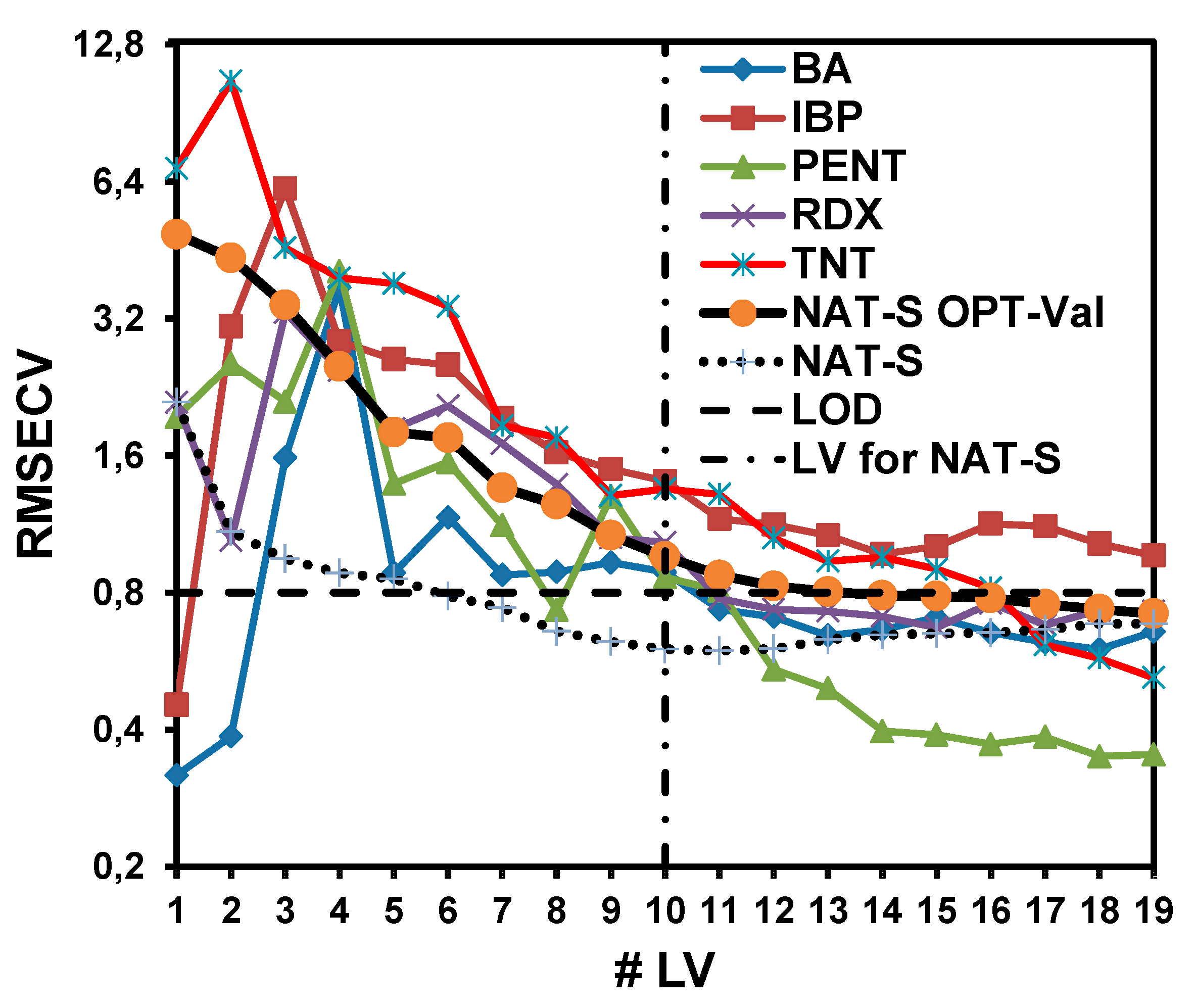
For the NAT-S OPT-Val model, 19 LV were required to obtain a good RMSECV value. Figure 5 shows the dependence of the RMSECV values for the prediction of each interference as a function of the LV. The NAT-S OPT-Val and NAT-S models were generated to determine how the RMSECV values decrease with the LV and compare the two models. The NAT-S model showed the minimum RMSECV at L = 10. Adding more LV resulted in worse RMSECV values. For the NAT-S OPT-Val model, the minimum RMSECV was achieved with 19 LV. Nevertheless, at 10 LV, the RMSECV values for other interferences were also sufficiently close to the RMSECV value for the model. For that reason, TNT and IBP interferences did not allow the RMSECV value of the NAT-S OPT-Val model to approach the RMSECV value of the NAT-S model.

3.2. Pattern Recognition Analysis

All sample spectra were normalized using VN preprocessing. Then, they were evaluated using Pre-CLS. The soil database used for the evaluation initially contained QCL reflectance spectra of four different natural soils, sand, and clay standards. It was expanded using linear combinations of sand and clay by applying the concept of Self-Simulated Learning Artificial Intelligence (SSLAI). SSLAI consists of an Artificial Intelligence method that uses minimal information to develop the Machine Learning models. In this case, other types of soils are simulated using those that are available, and these new simulated soils are used for the analysis. FSA algorithm for Pre-CLS was applied for spectra of the samples, and one spectrum of the database was added to the model (see Equation (7)) for most spectra. Next, the sum of ${\beta }_j$ (SUM(β)) parameters was calculated without including the bias (${\beta }_0$), and a simple binary discrimination model was generated and evaluated (see

Table 6. Confusion matrix and evaluation criteria for the binary discrimination model using SUM (β) parameters.

	Precision	Recall	F1-Score	Support	Accuracy	Matrix of Confusion
	Model					EXP	NONE
EXP	0.768	1.000	0.869	1126	0.877	865	261
NONE	1.000	0.793	0.884	997		0	997

) using this parameter to distinguish between contaminated and clean soils.

Figure 6a shows the probability distribution of SUM(β) for the two classes of the binary model. In this figure was observed a broad distribution of SUM(β) for the samples contaminated by explosives (EXP), it is due to the range of concentrations. Additionally, when samples EXP has the highest concentration of HEs, the value SUM(β) approaches 0 because it has the lowest proportion of soil. On the other hand, in the NONE sample, the distribution is sharpest, and the SUM(β) is highest.

The evaluation criteria (precision, recall, f1-score, and accuracy) and the confusion matrix for the model are shown in Table 6. This model has high precision in predicting clean soils (NONE), whereas it is moderate in predicting contaminated soils (EXP). This is because soils with low explosive concentrations are predicted as clean, increasing the number of false negatives. This happens at low concentrations (<2%), where the model does not work well.

Following the scheme illustrated in Figure 1, PCA was applied to the normalized data providing 20 principal components accounting for 99.99% of the variance. These components were normalized using an auto-scale preprocessing, and the SUM (β) was added as an additional principal component. Then, various ML methods were used to generate multi-classification models to discriminate between soils contaminated with three types of explosives (DNT, TNT, and RDX) and clean soil (NONE). These models were evaluated using accuracy and log-loss calculated over the test data (Figure 6b). The best method was RFC. This method constructs a multitude of decision trees during the training process and outputs the class that is the mode of the classes of the individual trees. The evaluation criteria (precision, recall, f1-score, and accuracy) and the confusion matrix calculated for the RFC model over the test data are listed in

Table 7. Confusion matrix and evaluation criteria for the random forest classification model.

	Precision	Recall	f1-Score	Support	Accuracy	Confusion Matrix
	Model					DNT	NONE	RDX	TNT
DNT	0.997	0.997	0.997	347	0.997	346	1	0	0
NONE	1.000	0.996	0.998	564		0	564	0	0
RDX	0.993	1.000	0.997	149		1	0	148	0
TNT	0.990	1.000	0.995	100		0	1	0	99
	Test					DNT	NONE	RDX	TNT
DNT	1.000	0.997	0.998	289	0.996	289	0	0	0
NONE	0.993	1.000	0.997	433		0	430	1	2
RDX	0.993	0.993	0.993	139		1	0	138	0
TNT	1.000	0.981	0.990	102		0	0	0	102

. The test data were classified almost entirely. Other strategies such as the generation of models without SUM (β) were also evaluated (data not shown); however, these provided poor results with a high number of false positives, i.e., many samples of clean soil were classified as containing explosives. This was resolved by adding the SUM (β) parameter.

4. Conclusions

This paper presented methods for quantifying DNT and detecting HEs in natural and synthetic soil matrices. The remote detection of HEs at a distance of 15 cm was achieved using multiple benefits of QCL spectroscopy, providing the evidence that it can be used in direct field applications. The obtained LOD values were adequate for the intended application. This study demonstrated that it is possible to get proper detection in the MIR range using diffuse reflection in the back-reflection mode for matrices containing components with low reflectivity such as soils. The remote detection of HEs in soils is now much more viable due to the high-power QCLs that are commercially available.

In the presented experiments, DNT signals could be observed in the spectra of solid mixtures with complex matrices, enabling the detection of explosives and quantification of DNT. For quantifying DNT in soil matrices, PLS models were useful for generating calibration curves. The best-performing models were obtained using VN preprocessing for all spectra. This preprocessing procedure proved to be suitable for samples, in which signals from analytes spectra overlapped with signals from matrices (natural soil, synthetic soil, and bentonite) spectra and relative intensity differences between spectra were small. In models that involved mixtures of explosives with KBr, VN preprocessing is not suitable because the KBr matrix does not have interfering signals in the spectroscopic window of interest. Therefore, this preprocessing step was not required. Hence, it can be concluded that VN is a useful preprocessing step for soil samples that have highly interfering matrices such as other explosives (TNT, RDX, and PETN) and non-explosives (BA and IBP). The strategy of adding samples of other analytes as possible interferences produced more selective models, making them more robust. The interferences used were organic compounds with many signals in the studied region. The interferences included explosives such as TNT, PETN, and RDX, as well as organic compounds such as BA and IBP. The NAT-S model was able to evade all interferences when it was trained with samples contaminated with these compounds. For the model to be accurate for other soils and possible interferences, it should be re-trained with corresponding samples.

Furthermore, an AI-based on an ML pipeline scheme (see Figure 1) was applied to obtain an RFC model for HEs detection in soil matrices. This scheme included Pre-CLS assisted by SSLAI and ML methods.

The expansion of the soil database generated by the linear combinations of QCL reflectance spectra of four different soils (natural soils, sand, and clay standards) allowed the application of Self-Simulated Learning Artificial Intelligence (SSLAI) concept. At the same time, it was possible to couple a simple forward selection algorithm (FSA) that facilitated the compression of the model when using simple multivariate analyses; CLS as additional preprocessing and PCA to reduce the number of spectral variables. Therefore, the combination of PCA, Pre-CLS, and SSLAI is an innovative ML pipeline that allows enriching the prediction of the model. Almost all tested samples of the studied soils and explosives (DNT, RDX, and TNT) were correctly classified by the model (see Table 7), providing an accuracy score of 0.996.

References

1. Frische, T.; Höper, H. Soil microbial parameters and luminescent bacteria assays as indicators for in situ bioremediation of TNT-contaminated soils. Chemosphere 2003, 50, 415–427. [Google Scholar] [CrossRef]
2. Correa-Torres, S.N.; Pacheco-Londono, L.C.; Espinosa-Fuentes, E.A.; Rodriguez, L.; Souto-Bachiller, F.A.; Hernandez-Rivera, S.P. TNT removal from culture media by three commonly available wild plants growing in the Caribbean. J. Environ. Monit. 2012, 14, 30–33. [Google Scholar] [CrossRef] [PubMed]
3. Hildenbrand, J.; Herbst, J.; Wöllenstein, J.; Lambrecht, A. Explosive detection using infrared laser spectroscopy. Proc. SPIE 2009, 7222, 72220B. [Google Scholar]
4. Narang, U.; Gauger, P.R.; Ligler, F.S. A Displacement Flow Immunosensor for Explosive Detection Using Microcapillaries. Anal. Chem. 1997, 69, 2779–2785. [Google Scholar] [CrossRef]
5. Hilmi, A.; Luong, J.H.T. Micromachined Electrophoresis Chips with Electrochemical Detectors for Analysis of Explosive Compounds in Soil and Groundwater. Environ. Sci. Technol. 2000, 34, 3046–3050. [Google Scholar] [CrossRef]
6. Kumar, S.; Venkatramaiah, N.; Patil, S. Fluoranthene Based Derivatives for Detection of Trace Explosive Nitroaromatics. J. Phys. Chem. C 2013, 117, 7236–7245. [Google Scholar] [CrossRef]
7. Sheremata, T.W.; Halasz, A.; Paquet, L.; Thiboutot, S.; Ampleman, G.; Hawari, J. The Fate of the Cyclic Nitramine Explosive RDX in Natural Soil. Environ. Sci. Technol. 2001, 35, 1037–1040. [Google Scholar] [CrossRef]
8. Larson, S.L.; Martin, W.A.; Escalon, B.L.; Thompson, M. Dissolution, Sorption, and Kinetics Involved in Systems Containing Explosives, Water, and Soil. Environ. Sci. Technol. 2008, 42, 786–792. [Google Scholar] [CrossRef]
9. Marple, R.L.; LaCourse, W.R. Application of Photoassisted Electrochemical Detection to Explosive-Containing Environmental Samples. Anal. Chem. 2005, 77, 6709–6714. [Google Scholar] [CrossRef]
10. Gallagher, N.B.; Blake, T.A.; Gassman, P.L. Application of extended inverse scatter correction to mid-infrared reflectance spectra of soil. J. Chemom. 2005, 19, 271–281. [Google Scholar] [CrossRef]
11. Forouzangohar, M.; Kookana, R.S.; Forrester, S.T.; Smernik, R.J.; Chittleborough, D.J. Mid-infrared Spectroscopy and Chemometrics to Predict Diuron Sorption Coefficients in Soils. Environ. Sci. Technol. 2008, 42, 3283–3288. [Google Scholar] [CrossRef]
12. Gallagher, N.B.; Gassman, P.L.; Blake, T.A. Strategies for Detecting Organic Liquids on Soils Using Mid-Infrared Reflection Spectroscopy. Environ. Sci. Technol. 2008, 42, 5700–5705. [Google Scholar] [CrossRef] [PubMed]
13. Mukherjee, A.; Von der Porten, S.; Patel, C.K.N. Standoff detection of explosive substances at distances of up to 150 m. Appl. Opt. 2010, 49, 2072–2078. [Google Scholar] [CrossRef]
14. Hernández, M.D.; Santiago, I.; Padilla, I.Y. Macro-sorption of 2,4-dinitrotoluene onto sandy and clay soils. Proc. SPIE 2006, 6217, 621736. [Google Scholar]
15. Baez, B.; Correa, S.N.; Hernandez-Rivera, S.P.; de Jesus, M.; Castro, M.E.; Mina, N.; Briano, J.G. Transport of explosives I: TNT in soil and its equilibrium vapor. Proc. SPIE 2004, 5415, 1389–1399. [Google Scholar]
16. Torres, A.; Padilla, I.; Hwang, S. Physical modeling of 2,4-DNT gaseous diffusion through unsaturated soil. Proc. SPIE 2007, 6553, 65531Q. [Google Scholar]
17. Herrera-Sandoval, G.M.; Ballesteros, L.M.; Mina, N.; Briano, J.; Castro, M.E.; Hernandez-Rivera, S.P. Raman signatures of TNT in contact with sand particles. Proc. SPIE 2005, 5794, 1245–1253. [Google Scholar]
18. Blanco, A.; Mina, N.; Castro, M.E.; Castillo-Chara, J.; Hernandez-Rivera, S.P. Effect of environmental conditions on the spectroscopic signature of DNT in sand. Proc. SPIE 2005, 5794, 1281–1289. [Google Scholar]
19. Ballesteros, L.M.; Herrera, G.M.; Castro, M.E.; Briano, J.; Mina, N.; Hernandez-Rivera, S.P. Spectroscopic signatures of PETN in contact with sand particles. Proc. SPIE 2005, 5794, 1254–1262. [Google Scholar]
20. Hernandez-Rivera, S.P.; Manrique-Bastidas, C.A.; Blanco, A.; Primera, O.M.; Pacheco, L.C.; Castillo-Chara, J.; Castro, M.E.; Mina, N. Spectroscopic characterization of nitroaromatic landmine signature explosives. Proc. SPIE 2004, 5415, 474–485. [Google Scholar]
21. Osorio, C.; Gomez, L.M.; Hernandez, S.P.; Castro, M.E. Time-of-flight mass spectroscopy measurements of TNT and RDX on soil surfaces. Proc. SPIE 2005, 5794, 803–811. [Google Scholar]
22. Manrique-Bastidas, C.A.; Mina, N.; Castro, M.E.; Hernandez-Rivera, S.P. Raman microspectroscopy and FTIR crystallization studies of 2,4,6-TNT in soil. Proc. SPIE 2005, 5794, 1358–1365. [Google Scholar]
23. Blanco, A.; Pacheco-Londoño, L.C.; Peña-Quevedo, A.J.; Hernández-Rivera, S.P. UV Raman detection of 2,4-DNT in contact with sand particles. Proc. SPIE 2006, 6217, 621737. [Google Scholar]
24. Galán-Freyle, N.J.; Pacheco-Londoño, L.C.; Figueroa-Navedo, A.M.; Hernandez-Rivera, S.P. Standoff Detection of Highly Energetic Materials Using Laser-Induced Thermal Excitation of Infrared Emission. Appl. Spectrosc. 2015, 69, 535–544. [Google Scholar] [CrossRef] [PubMed]
25. Galán-Freyle, N.J.; Ospina-Castro, M.L.; Medina-González, A.R.; Villarreal-González, R.; Hernández-Rivera, S.P.; Pacheco-Londoño, L.C. Artificial Intelligence Assisted Mid-Infrared Laser Spectroscopy In Situ Detection of Petroleum in Soils. Appl. Sci. 2020, 10, 1319. [Google Scholar] [CrossRef] [Green Version]
26. Rüther, A.; Pfeifer, M.; Lórenz-Fonfría, V.A.; Lüdeke, S. pH Titration Monitored by Quantum Cascade Laser-Based Vibrational Circular Dichroism. J. Phys. Chem. B 2014, 118, 3941–3949. [Google Scholar] [CrossRef]
27. Lüdeke, S.; Pfeifer, M.; Fischer, P. Quantum-Cascade Laser-Based Vibrational Circular Dichroism. J. Am. Chem. Soc. 2011, 133, 5704–5707. [Google Scholar] [CrossRef]
28. Shi, Q.; Nelson, D.D.; McManus, J.B.; Zahniser, M.S.; Parrish, M.E.; Baren, R.E.; Shafer, K.H.; Harward, C.N. Quantum Cascade Infrared Laser Spectroscopy for Real-Time Cigarette Smoke Analysis. Anal. Chem. 2003, 75, 5180–5190. [Google Scholar] [CrossRef]
29. Wörle, K.; Seichter, F.; Wilk, A.; Armacost, C.; Day, T.; Godejohann, M.; Wachter, U.; Vogt, J.; Radermacher, P.; Mizaikoff, B. Breath Analysis with Broadly Tunable Quantum Cascade Lasers. Anal. Chem. 2013, 85, 2697–2702. [Google Scholar] [CrossRef]
30. Galán-Freyle, N.J.; Pacheco-Londoño, L.C.; Román-Ospino, A.D.; Hernandez-Rivera, S.P. Applications of Quantum Cascade Laser Spectroscopy in the Analysis of Pharmaceutical Formulations. Appl. Spectrosc. 2016, 70, 1511–1519. [Google Scholar] [CrossRef]
31. Padilla-Jiménez, A.C.; Ortiz-Rivera, W.; Rios-Velazquez, C.; Vazquez-Ayala, I.; Hernández-Rivera, S.P. Detection and discrimination of microorganisms on various substrates with quantum cascade laser spectroscopy. OPTICE 2014, 53, 061611. [Google Scholar] [CrossRef]
32. Faist, J.; Capasso, F.; Sivco, D.L.; Sirtori, C.; Hutchinson, A.L.; Cho, A.Y. Quantum Cascade Laser. Science 1994, 264, 553–556. [Google Scholar] [CrossRef] [PubMed]
33. Hvozdara, L.; Pennington, N.; Kraft, M.; Karlowatz, M.; Mizaikoff, B. Quantum cascade lasers for mid-infrared spectroscopy. Vib. Spectrosc. 2002, 30, 53–58. [Google Scholar] [CrossRef]
34. Ruiz-Caballero, J.L.; Blanco-Riveiro, L.A.; Ramirez-Marrero, I.A.; Perez-Almodovar, L.A.; Colon-Mercado, A.M.; Castro-Suarez, J.R.; Pacheco-Londoño, L.C.; Hernandez-Rivera, S.P. Enhanced RDX Detection Studies on Various Types of Substrates via Tunable Quantum Cascade Laser Spectrometer Coupled with Grazing Angle Probe. IOP Conf. Ser. Mater. Sci. Eng. 2019, 519, 012007. [Google Scholar] [CrossRef]
35. Pacheco-Londoño, L.C.; Galán-Freyle, N.J.; Figueroa-Navedo, A.M.; Infante-Castillo, R.; Ruiz-Caballero, J.L.; Hernández-Rivera, S.P. Quantum cascade laser back-reflection spectroscopy at grazing-angle incidence using the fast Fourier transform as a data preprocessing algorithm. J. Chemom. 2019, 33, e3167. [Google Scholar] [CrossRef]
36. Pacheco-Londoño, L.C.; Aparicio-Bolaño, J.A.; Galán-Freyle, N.J.; Román-Ospino, A.D.; Ruiz-Caballero, J.L.; Hernández-Rivera, S.P. Classical Least Squares-Assisted Mid-Infrared (MIR) Laser Spectroscopy Detection of High Explosives on Fabrics. Appl. Spectrosc. 2019, 73, 17–29. [Google Scholar] [CrossRef]
37. Pacheco-Londoño, L.C.; Ruiz-Caballero, J.L.; Ramírez-Cedeño, M.L.; Infante-Castillo, R.; Gálan-Freyle, N.J.; Hernández-Rivera, S.P. Surface Persistence of Trace Level Deposits of Highly Energetic Materials. Molecules 2019, 24, 3494. [Google Scholar] [CrossRef] [Green Version]
38. Pacheco-Londoño, L.C.; Castro-Suarez, J.R.; Galán-Freyle, N.J.; Figueroa-Navedo, A.M.; Ruiz-Caballero, J.L.; Infante-Castillo, R.; Hernández-Rivera, S.P. Mid-Infrared Laser Spectroscopy Applications I: Detection of Traces of High Explosives on Reflective and Matte Substrates. In Infrared Spectroscopy—Principles, Advances, and Applications; IntechOpen: London, UK, 2019. [Google Scholar] [CrossRef] [Green Version]
39. Phillips, M.C.; Bernacki, B.E. Hyperspectral microscopy of explosives particles using an external cavity quantum cascade laser. OPTICE 2012, 52, 061302. [Google Scholar] [CrossRef] [Green Version]
40. Pacheco-Londoño, L.C.; Castro-Suarez, J.R.; Hernández-Rivera, S.P. Detection of Nitroaromatic and Peroxide Explosives in Air Using Infrared Spectroscopy: QCL and FTIR. Adv. Opt. Technol. 2013, 2013, 532670. [Google Scholar] [CrossRef] [Green Version]
41. Sirkeli, V.P.; Yilmazoglu, O.; Preu, S.; Küppers, F.; Hartnagel, H.L. Proposal for a Monolithic Broadband Terahertz Quantum Cascade Laser Array Tailored to Detection of Explosive Materials. Sens. Lett. 2018, 16, 1–7. [Google Scholar] [CrossRef]
42. Pettersson, A.; Wallin, S.; Östmark, H.; Ehlerding, A.; Johansson, I.; Nordberg, M.; Ellis, H.; Al-Khalili, A. Explosives standoff detection using Raman spectroscopy: From bulk towards trace detection. Proc. SPIE 2010, 7664, 76641K. [Google Scholar]
43. Yang, C.S.C.; Brown, E.E.; Hommerich, U.; Jin, F.; Trivedi, S.B.; Samuels, A.C.; Snyder, A.P. Long-Wave, Infrared Laser-Induced Breakdown (LIBS) Spectroscopy Emissions from Energetic Materials. Appl. Spectrosc. 2012, 66, 1397–1402. [Google Scholar] [CrossRef]
44. Misra, A.K.; Sharma, S.K.; Acosta, T.E.; Porter, J.N.; Bates, D.E. Single-Pulse Standoff Raman Detection of Chemicals from 120 m Distance During Daytime. Appl. Spectrosc. 2012, 66, 1279–1285. [Google Scholar] [CrossRef]
45. Gottfried, J.L.; De Lucia, F.C.; Munson, C.A.; Miziolek, A.W. Standoff Detection of Chemical and Biological Threats Using Laser-Induced Breakdown Spectroscopy. Appl. Spectrosc. 2008, 62, 353–363. [Google Scholar] [CrossRef] [PubMed]
46. Castro-Suarez, J.R.; Pacheco-Londoño, L.C.; Vélez-Reyes, M.; Diem, M.; Tague, T.J.; Hernandez-Rivera, S.P. FT-IR Standoff Detection of Thermally Excited Emissions of Trinitrotoluene (TNT) Deposited on Aluminum Substrates. Appl. Spectrosc. 2013, 67, 181–186. [Google Scholar] [CrossRef] [PubMed]
47. Carter, J.C.; Angel, S.M.; Lawrence-Snyder, M.; Scaffidi, J.; Whipple, R.E.; Reynolds, J.G. Standoff Detection of High Explosive Materials at 50 Meters in Ambient Light Conditions Using a Small Raman Instrument. Appl. Spectrosc. 2005, 59, 769–775. [Google Scholar] [CrossRef] [PubMed]
48. Averett, L.A.; Griffiths, P.R. Mid-Infrared Diffuse Reflection of a Strongly Absorbing Analyte on Non-Absorbing and Absorbing Matrices. Part II: Thin Liquid Layers on Powdered Substrates. Appl. Spectrosc. 2008, 62, 383–388. [Google Scholar] [CrossRef]
49. Pacheco-Londoño, L.; Ortiz-Rivera, W.; Primera-Pedrozo, O.; Hernández-Rivera, S. Vibrational spectroscopy standoff detection of explosives. Anal. Bioanal. Chem. 2009, 395, 323–335. [Google Scholar] [CrossRef]
50. Van Neste, C.W.; Senesac, L.R.; Thundat, T. Standoff Spectroscopy of Surface Adsorbed Chemicals. Anal. Chem. 2009, 81, 1952–1956. [Google Scholar] [CrossRef]
51. Moros, J.; Lorenzo, J.A.; Lucena, P.; Miguel Tobaria, L.; Laserna, J.J. Simultaneous Raman Spectroscopy−Laser-Induced Breakdown Spectroscopy for Instant Standoff Analysis of Explosives Using a Mobile Integrated Sensor Platform. Anal. Chem. 2010, 82, 1389–1400. [Google Scholar] [CrossRef]
52. Moros, J.; Laserna, J.J. New Raman–Laser-Induced Breakdown Spectroscopy Identity of Explosives Using Parametric Data Fusion on an Integrated Sensing Platform. Anal. Chem. 2011, 83, 6275–6285. [Google Scholar] [CrossRef] [PubMed]
53. Ortiz-Rivera, W.; Pacheco-Londoño, L.; Castro-Suarez, J.; Felix-Rivera, H.; Hernandez-Rivera, S. Vibrational Spectroscopy Standoff Detection of Threat Chemicals; SPIE: Bellingham, WA, USA, 2011; Volume 8031. [Google Scholar]
54. Miyazawa, M.; Pavan, M.A.; de Oliveira, E.L.; Ionashiro, M.; Silva, A.K. Gravimetric determination of soil organic matter. Braz. Arch. Biol. Technol. 2000, 43, 475–478. [Google Scholar] [CrossRef]
55. Weiner, E.R. Applications of Environmental Chemistry: A Practical Guide for Environmental Professionals; Lewis Pub.: Boca Raton, FL, USA, 2000. [Google Scholar]
56. Yanjun, C.; Achari, G.; Langford, C.H. Protocols for the analysis of transformer oil and its degradation in soil by hydrogen peroxide. Can. J. Civ. Eng. 2009, 36, 1547–1557. [Google Scholar] [CrossRef]
57. Lorber, A. Error propagation and figures of merit for quantification by solving matrix equations. Anal. Chem. 1986, 58, 1167–1172. [Google Scholar] [CrossRef]
58. Ferreira, M.H.; Braga, J.W.B.; Sena, M.M. Development and validation of a chemometric method for direct determination of hydrochlorothiazide in pharmaceutical samples by diffuse reflectance near-infrared spectroscopy. Microelectron. J. 2013, 109, 158–164. [Google Scholar] [CrossRef]
59. Olivieri, A.C.; Faber, N.M.; Ferré, J.; Boqué, R.; Kalivas, J.H.; Mark, H. Uncertainty estimation and figures of merit for multivariate calibration (IUPAC Technical Report). Pure Appl. Chem. 2006, 78, 633. [Google Scholar] [CrossRef] [Green Version]
60. Felipe-Sotelo, M.; Cal-Prieto, M.J.; Ferre, J.; Boque, R.; Andrade, J.M.; Carlosena, A. Linear PLS regression to cope with interferences of major concomitants in the determination of antimony by ETAAS. J. Anal. Spectrom. 2006, 21, 61–68. [Google Scholar] [CrossRef]
61. Galan-Freyle, N.J.; Figueroa-Navedo, A.M.; Pacheco-Londoño, Y.C.; Ortiz-Rivera, W.; Pacheco-Londoño, L.C.; Hernández-Rivera, S.P. Chemometrics-enhanced fiber-optic Raman detection, discrimination and quantification of chemical agents simulants concealed in commercial bottles. Anal. Chem. Res. 2014, 2, 15–22. [Google Scholar] [CrossRef] [Green Version]
62. Buitinck, L.; Louppe, G.; Blondel, M.; Pedregosa, F.; Mueller, A.; Grisel, O.; Niculae, V.; Prettenhofer, P.; Gramfort, A.; Grobler, J.; et al. API design for machine learning software: Experiences from the scikit-learn project. In Proceedings of the European Conference on Machine Learning and Principles and Practices of Knowledge Discovery in Databases, Prague, Czech Republic, 23 September 2013. [Google Scholar]
63. Kubelka, P. New Contributions to the Optics of Intensely Light-Scattering Materials. Part I. J. Opt. Soc. Am 1948, 38, 448. [Google Scholar] [CrossRef]
64. Bull, C.R. Compensation for particle size effects in near-infrared reflectance. Analyst 1991, 116, 781–786. [Google Scholar] [CrossRef]
65. Sirita, J.; Phanichphant, S.; Meunier, F.C. Quantitative Analysis of Adsorbate Concentrations by Diffuse Reflectance FT-IR. Anal. Chem. 2007, 79, 3912–3918. [Google Scholar] [CrossRef] [PubMed] [Green Version]
66. Igne, B.; Hurburgh, C.R. Local chemometrics for samples and variables: Optimizing calibration and standardization processes. J. Chemom. 2010, 24, 75–86. [Google Scholar] [CrossRef]
Figure 1. Machine learning pipeline for improving classification.
Applsci 10 04178 g001
Figure 2. Predicted values vs. real values of % DNT from partial least squares (PLS) models on the matrices: (a) bentonite clay (BC); (b) synthetic soil (SYN-S); (c) natural soil (NAT-S); (d) NAT-S to low concentration (NAT-S Low); (e) potassium bromide (KBr) and (f) KBr to low concentration (KBr Low).
Applsci 10 04178 g002
Figure 3. DNT spectrum in the investigated soil matrices in K-M (K-M for T: K-M calculate from transmittance for red spectra): (a) BC; (b) SYN-S; (c) NAT-S, and (d) NAT-S Low.
Applsci 10 04178 g003
Figure 4. Predictions for 100 pts. maps after applying VN, mean centering (MC), and no preprocessing: (a) simple mixture (NAT-S-M); (b) macerating the components (NAT-S-MM); (c) Averages for the predictions of NAT-S-M and NAT-S-MM (d) NAT2-S with VN preprocessing.
Applsci 10 04178 g004
Figure 5. Dependence of the root-mean-square error of cross-validation (RMSECV) on LV for the considered interferences: the NAT-S optimization of the validation set (OPT-Val) and NAT-S models.
Applsci 10 04178 g005
Figure 6. (a) Probability distribution of the sum of β j (SUM (β)) for a simple binary discrimination model. (b) Comparison of the tested machine learning (ML) methods in terms of their log-loss and accuracy.
Applsci 10 04178 g006