Determination of Necessary Subsidiary Track According to Train Operation Frequency in a Heterogeneous Train Pattern

Abstract

In this study, a genetic algorithm was used to calculate the scheduled waiting time according to the train operation frequency of heterogeneous trains operating on one track. The acquired data were then used to determine the appropriate subsidiary track at which high-speed trains can load or release cargo away from low-speed trains. A metaheuristic genetic algorithm was applied and implemented using Javascript/jQuery. Six cases were investigated, which provided values of subsidiary track that vary according to the operation frequencies of different types of trains, and solutions were derived through 100 simulations using a stochastic method. The analysis results showed that the train overtaking frequency was the highest at the third intermediate station within the simulation, suggesting that this particular station requires a subsidiary track, even if the operating frequency of each train differs across the entire track considered in this study. The results of this study are expected to facilitate objective and practical planning during railway construction.

1. Introduction

The goal of railway construction is the transportation of passengers and freight, and train operation lies at the core of this transportation. To transport passengers and freight, an optimal operation plan is required under the given conditions with a transportation system that systematically combines various components such as construction, vehicles, and signals [1]. In South Korea, train operation plans are established using construction documents when constructing railway tracks during the construction design phase. Train operation plans are also addressed in preliminary feasibility studies, but these studies only consider the rough train operation plan.

To consider the operation of heterogeneous train traffic in the railroad line construction plan, an operation pattern is generated, which is used to evaluate overtaking between trains. The overtaking or passing of one train by another is evaluated depending on the type of train considered, the stopping time, the number of stopping stations, and the speed of the trains. The station design is determined based on this operation pattern. If a low-speed train must be moved out of the path of an incoming high-speed train (this process will be referred to as evacuation, hereinafter), the train operation time inevitably increases. If a station that has a subsidiary track for the low-speed train is not at an appropriate distance, the headway between the high-speed and low-speed trains or the exit time of the low-speed train from the path of the high-speed train increases.

This increase in the headway between trains and the time to remove the low-speed train from the path of the high-speed train is closely related not only to the train operation time and service level but also to the track capacity. According to the International Union of Railways (UIC), many railways around the world are constructed to provide train services required for infrastructure, and as part of this effort, the allocation and utilization of railway capacity is more important than ever [2]. However, if the goal is to install a subsidiary track at every station to improve the train operation service, the project cost will increase and the feasibility of improving the operation will reduce.

In the past, the waiting time of trains in a train network was used mainly in the research of delay transfer for late and following trains. However, a second category of waiting time, called the scheduled waiting time, is calculated for railway networks. The scheduled waiting time, like delay, occurs in the train scheduling process and does not affect the operation of other trains [3]. The present study explicitly analyzed and derived the effects of heterogeneous train operation frequency and the existence or absence of a subsidiary track on the weighted scheduled waiting time for a train schedule where overtaking and evacuation occur when heterogeneous trains are operated on the same track. To analyze the location of the subsidiary track with the scheduled waiting time, a metaheuristics algorithm was applied. The results of this study can be used to facilitate objective and practical planning during railway construction.

1.1. Metaheuristic Method

Heuristic methods are generally applied to untangle representative non-deterministic polynomial-time (NP)-hard problems. Heuristics generally refer to “specific heuristics” designed to be appropriate for unraveling a specific type of problem. Metaheuristics refer to advanced heuristics and a universal algorithm framework that provides guidelines on general structures and strategies for building specific heuristics. In short, metaheuristics are upper-level heuristics that can be used as a basic framework of an algorithm when developing heuristics [4,5,6,7].

Since the mid-1960s, various metaheuristic algorithms have been proposed, and their application programs have also been increasing [8,9,10,11].

Table 1. Classification of Metaheuristics [8,16,17,18].

Categorization	Metaheuristics	Developer
Nature’s Evolutionary Process	Evolution Strategy	Schwefel
	Evolution Programming	Rechenberg
	Genetic Algorithm	Fogel, Owens, and Walsh
	Genetic Programming	Holland and Koza
	Differential Evolution	Storn and Price
Swarm	Ant Colony Optimization	Dorigo
	Particle Swarm Optimization	Kennedy and Eberhart
	Bee Colony Optimization	Lucic and Teodorovic
	Artificial Bee Colony	Karaboga
Natural and Social Phenomena	Simulated Annealing	Kirkpatrick
	Tabu Search	Glover
	Harmony Search	Geem et al.
Systematic Iteration	Iterated Local Search	Baxter
	Variable Neighborhood Search	Mladenovic and Hansen
	Guided Local Search	Voudouris

lists the major metaheuristic algorithms, which can be classified into: (a) evolution algorithms that imitate the evolution process of nature, (b) algorithms that imitate the behaviors of swarming living things, (c) algorithms that imitate natural and social phenomena, and (d) algorithms for finding neighbors through systematic iteration [4,8,9,10,11]. The evolution algorithms that imitate the evolution of nature, including genetic algorithms, generally involve methods that apply multiple evolutionary mechanisms to the design or implementation of a calculation model for solving a problem [12,13,14]. In addition to genetic algorithms, there are evolution strategies, evolution programming, and genetic programming. These methods imitate the conceptual evolutionary process based on natural selection and the law of inheritance [6]. The evolution algorithm is a stochastic process that generates a better result for finding a solution than a random search technique [4,8]. Algorithms that imitate natural and social phenomena use one solution for a periphery search technique, such as taboo search and simulation annealing, whereas the genetic algorithm uses a group of potential solutions [15]. The genetic algorithm continuously searches for a space of solutions by applying natural selection and the law of inheritance to the solutions of a generation [8].

The genetic algorithm can solve optimization or decision-making problems because its concepts and theory are simple, and it has demonstrated excellent performance when searching for numerous random solutions set by researchers [19,20]. In particular, the genetic algorithm is appropriate for solving problems with many variables and constraints because of its excellent search function in a complex solution space [8]. Furthermore, the high flexibility of this model provides the advantage of facilitating the addition of constraints and the modification of the objective function [4,8]. In the present research, a genetic algorithm is applied as a metaheuristic method to determine the necessary subsidiary track.

1.2. Genetic Algorithm

Rechenberg proposed an evolution strategy in 1965 [13]. Then, Fogel, Owens, and Walsh proposed evolution programming in 1966 [7]. Subsequently, the genetic algorithm was established by Holland in 1975, and it is a representative method based on the principle of evolution for solving problems. The genetic algorithm has been applied to diverse optimization and decision-making problems in engineering, natural science, business administration, and social sciences because it has a simple concept and theoretical base and provides excellent solution search function [4]. In particular, the genetic algorithm is appropriate for solving significantly difficult mathematical problems with many variables and constraints because it shows excellent search performance in a complex solution space [4]. Another advantage of the genetic algorithm is that the high flexibility of the model application makes it easy to add constraints and an objective function [8,21,22,23].

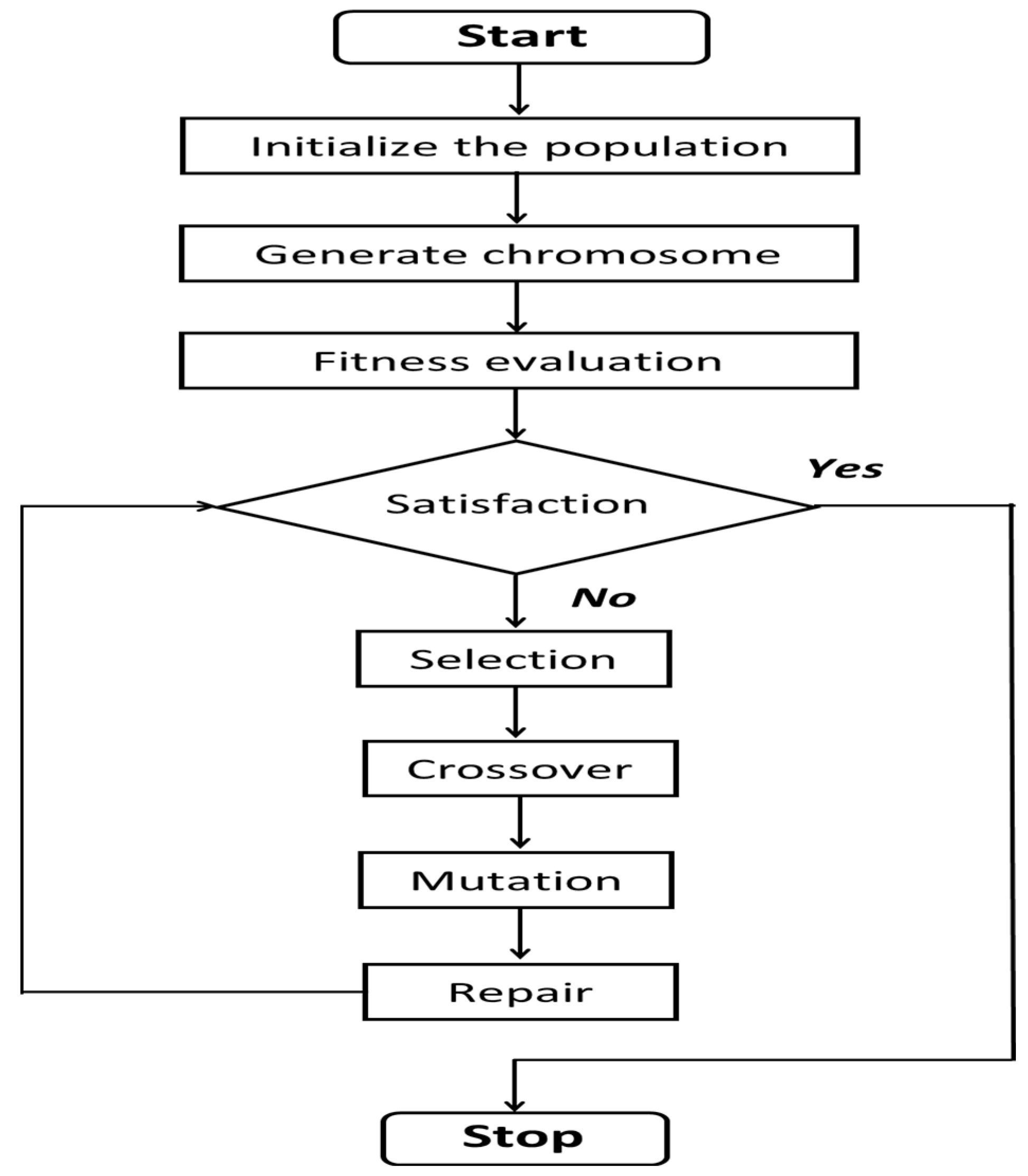
The genetic algorithm continuously reiterates the following process until the best solution is found: (a) generation of initial chromosome population, (b) chromosome coding, (c) chromosome mating and mutation (genetic manipulation), (d) health evaluation, (e) selection, (f) generation of a new chromosome group, and (g) determination of whether new chromosomes are stopped, mated, or mutated [8]. The first step of the genetic algorithm is to represent a potential solution to the problem as an entity. Because the actual representation affects other processes, it must accurately reflect the characteristics of the problem [8]. In the present study, the chromosomes comprise train types instead of separate trains when the genetic algorithm is implemented. Because real train planning is completed after reiterating the plan for each train type for the required number of times, it does not significantly influence the solution performance even if the train pattern is repeated. In this present study, train-type-based representations are used to reduce the searching time of the solution and reduce the number of decision-making parameters within an appropriate limit.

1.3. Summary of Related Studies

Many studies have been conducted to find the optimal solution of a train operation plan by applying genetic algorithms. Genetic algorithms have been applied to minimize the scheduled waiting time, train operation frequency, and timetable arrays. Wegele and Schneider suggested a genetic algorithm to compose a timetable [21]. They aimed to simplify the train transportation process by providing an optimization algorithm that can define optimization tasks to automatically control the train operation process and minimize customer discomfort caused by issues such as train delays. Gholami and Sotskov proposed a genetic algorithm for specifying and reserving the paths of trains developed to achieve efficient and powerful railroad tracks and timetables [24]. They suggested changing the trains’ starting times to find better times to begin train operation, lower delay, and to minimize the total operation time as much as possible. A method of applying the genetic algorithm to analyze the optimization of train operation frequency was proposed by Nirmala and Ramprasad [25]. They analyzed the solutions of the problem through two-level optimization, which determines the minimum train operation frequency required for each path and summarizes the operation frequency of each line. Liu and Dessouky investigated the passenger and freight train operation planning problem using a heuristics algorithm [26]. The goal of the studies mentioned above was to jointly solve passenger and freight train schedules when the same track is shared to enhance the efficiency of freight trains and to shorten the transportation time while maintaining the passenger train schedule in the same railway network. Furthermore, as shown in the above discussion, the genetic algorithm has been applied to optimize the number of operating trains and timetable arrays. Railway planners involved in constructing or upgrading railway infrastructure develop station layouts according to the train operation schedule primarily manually based on their experiences. However, determining the location of subsidiary tracks with train schedules is a very fastidious and complex problem because of various constraints such as the vehicle performance, signal system, and distance between stations [8]. This study aims to provide more practical analysis data rather than providing probable data of the planner. This is achieved by analyzing the weighted scheduled waiting time according to the train operation frequency and operation times in train schedules where overtaking and evacuation occur when three types of trains operate on the same track. Our objective and practical results can then be applied to appropriately select the placement of subsidiary tracks during railway and train operation planning. In this research, the scheduled waiting time should be considered in order to determine the positions of the subsidiary tracks. The scheduled waiting time is calculated when a preceding low-speed train waits for overtaking a follow-up high-speed train at a certain position. The certain position is the position of the subsidiary tracks in this research. Therefore, the scheduled waiting time should be mentioned to achieve the objective of this research.

2. Scheduled Waiting Time

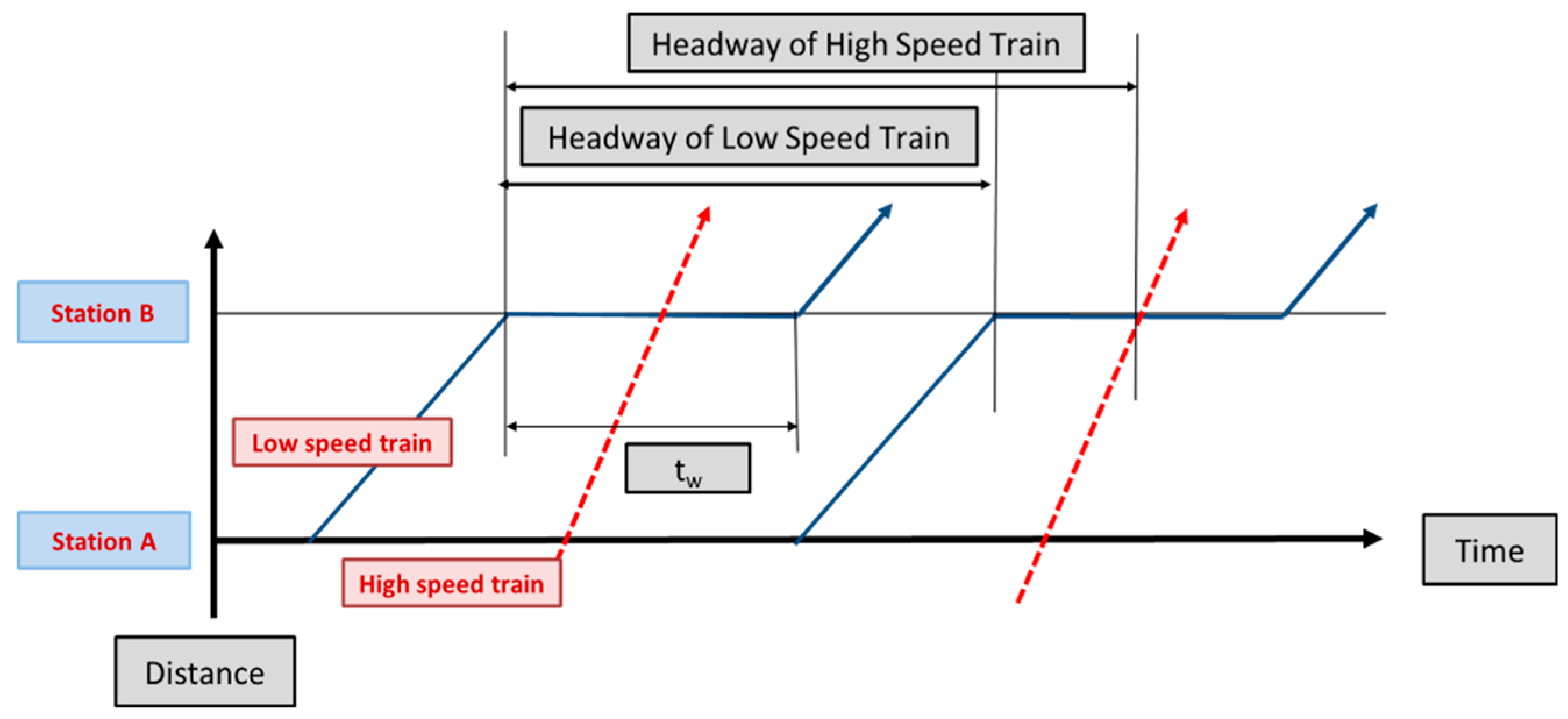
The scheduled waiting time implies an artificial increase of the total train operation time to solve interferences between trains during train operation. This occurs when heterogeneous trains operate on the identical railroad track [27]. The scheduled waiting times are not affected by the number of trains because with more trains, the longer the evacuation time of low-speed trains. Figure 1 shows a time–distance graph representing a route where two trains with different speeds compete at a station [28].

(t_w) denotes the waiting time of a low speed train due to overtaking a high-speed train at station B. This waiting time is referred to as the “scheduled waiting time” because it is already included in the train operation schedule. Waiting time is generated when passenger and freight trains with different speeds compete during operation. The scheduled waiting time generally increases the total operation and stopping times. When the entire route is changed from the arrival or departure stations of the train, the total transportation time does not always increase. The waiting time model of the scheduled waiting time is expressed as:

$$t_w=f\left(n_{tr}\right)$$

(1)

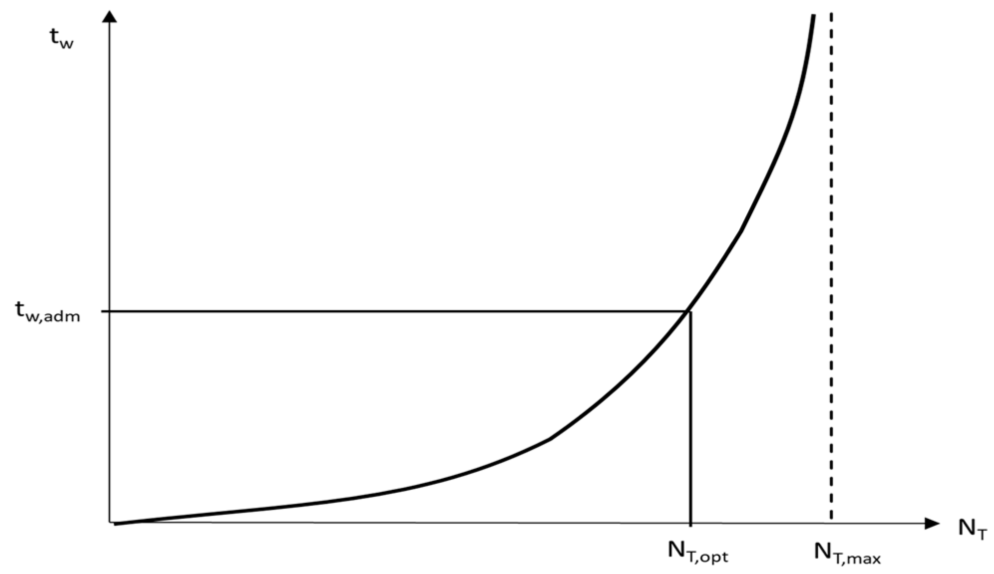
which represents a basic curve for the waiting time function. Here, n_Tr is the train operation frequency and is plotted in Figure 2.

In Figure 2, N_T,max represents the theoretical maximum track capacity, where (N_T) denotes the number of trains. When operating heterogeneous trains on one track, the theoretical maximum track capacity can be calculated by grouping and operating trains of the same type together. However, this method leads to poor train operation service and is not the goal of practical train operation. t_w,adm represents the allowance level of the scheduled waiting time. Once this is determined, we can specify the actual track capacity N_T,opt. The allowed waiting time is derived for the specified train operation pattern, that is, the operation of heterogeneous trains on one track. In a situation where one train is evacuated for another train at a specific station, that is, the transportation mode is changed, the modal shift has a significant effect on the waiting time of passengers or freight. When heterogeneous trains use the same track, the minimum headway for train j following train i is represented as t_h,i,j, which can be represented in the following matrix form,

$$T=\left(t_{h,i,j}\right)=\left[\begin{array}{ccc}{t}_{h,1,1}& t_{h,1,2}& \cdots \\ t_{h,2,1}& t_{h,2,2}& \cdots \\ \begin{array}{c}⋮\\ t_{h,n,1}\end{array}& \begin{array}{c}⋮\\ t_{h,n,2}\end{array}& \begin{array}{c}\ddots \\ \cdots \end{array}\end{array} \begin{array}{c}{t}_{h,1,n}\\ t_{h,2,n}\\ \begin{array}{c}⋮\\ t_{h,n,n}\end{array}\end{array}\right]$$

(2)

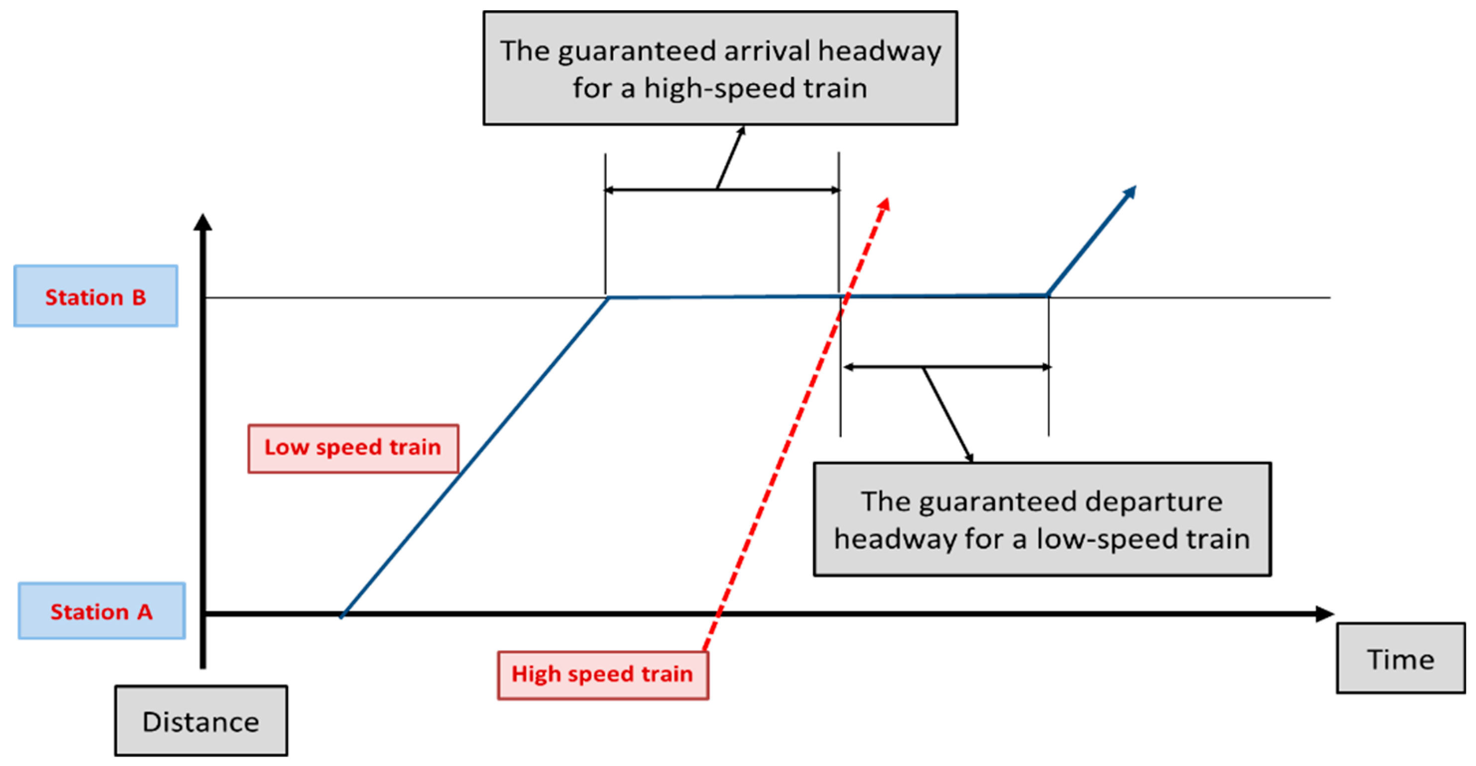
The types of trains considered in this study were high-speed, passenger, and freight trains. A freight train generates a scheduled waiting time by evacuating for a high-speed train and a passenger train. A passenger train generates a scheduled waiting time by evacuating for a high-speed train. It was assumed that overtaking was impossible between stations for all trains because too many operation patterns need to be considered, and it does not represent the practical operating conditions. Furthermore, arrival and departure headways are required to analyze the scheduled waiting times of passenger and freight trains evacuating to the subsidiary track under the precondition that high-speed, passenger, and freight trains operate on the same track. When a high-speed train catches up with a leading low-speed train (passenger or freight train), we need the headway for the high-speed train to arrive at the station without deceleration of the leading low-speed train and the departure headway of the low-speed train after the high-speed train has passed. Figure 3 shows the safe train separation distance between a high-speed train and a low-speed train at the station. This headway for each train is crucial when calculating the scheduled waiting time.

If the arrival headway of the high-speed train and the departure headway of the low-speed train increase, the total operation time of the low-speed train increases, which is not suitable for train operation. The track capacity also increases in this case. When a high-speed train (t_h), a passenger train (t_p), or a freight train (t_f) arrives at the n^th station (a_n), the headway H_w of train j following train i is represented by the following equations:

$$a_{n}Hw{t}_{i,j}^{p,h}=\left\{x : \left|a_n{t}_j^h-a_n{t}_i^p\right|\le Hw{t}_{i,j}^{p,h}\right\}$$

(3)

$$a_{n}Hw{t}_{i,j}^{f,h}=\left\{x : \left|a_n{t}_j^h-a_n{t}_i^f\right|\le Hw{t}_{i,j}^{f,h}\right\}$$

(4)

$$a_{n}Hw{t}_{i,j}^{f,p}=\left\{x : \left|a_n{t}_j^p-a_n{t}_i^f\right|\le Hw{t}_{i,j}^{f,p}\right\}$$

(5)

When each train departs from the n^th station (d_n), the headway H_w of train j following train i is expressed as:

$$d_{n}Hw{t}_{i,j}^{h,p}=\left\{x : \left|d_n{t}_j^p-d_n{t}_i^h\right|\le Hw{t}_{i,j}^{h,p}\right\}$$

(6)

$$d_{n}Hw{t}_{i,j}^{h,f}=\left\{x : \left|d_n{t}_j^f-d_n{t}_i^h\right|\le Hw{t}_{i,j}^{h,f}\right\}$$

(7)

$$d_{n}Hw{t}_{i,j}^{p,f}=\left\{x : \left|d_n{t}_j^f-d_n{t}_i^p\right|\le Hw{t}_{i,j}^{p,f}\right\}$$

(8)

When a high-speed train overtakes a preceding low-speed train (passenger or freight trains), the guaranteed arrival headway of the high-speed train without reduction of speed by a preceding low-speed train and the guaranteed departure headway of the low-speed train after passing the high-speed train are represented by Equations (3)–(8) [8]. By subtracting the arrival and departure times of the preceding train from the arrival and departure times of the subsequent train, respectively, the headway for the arrival and departure times of the preceding train and the following train can be estimated at the station.

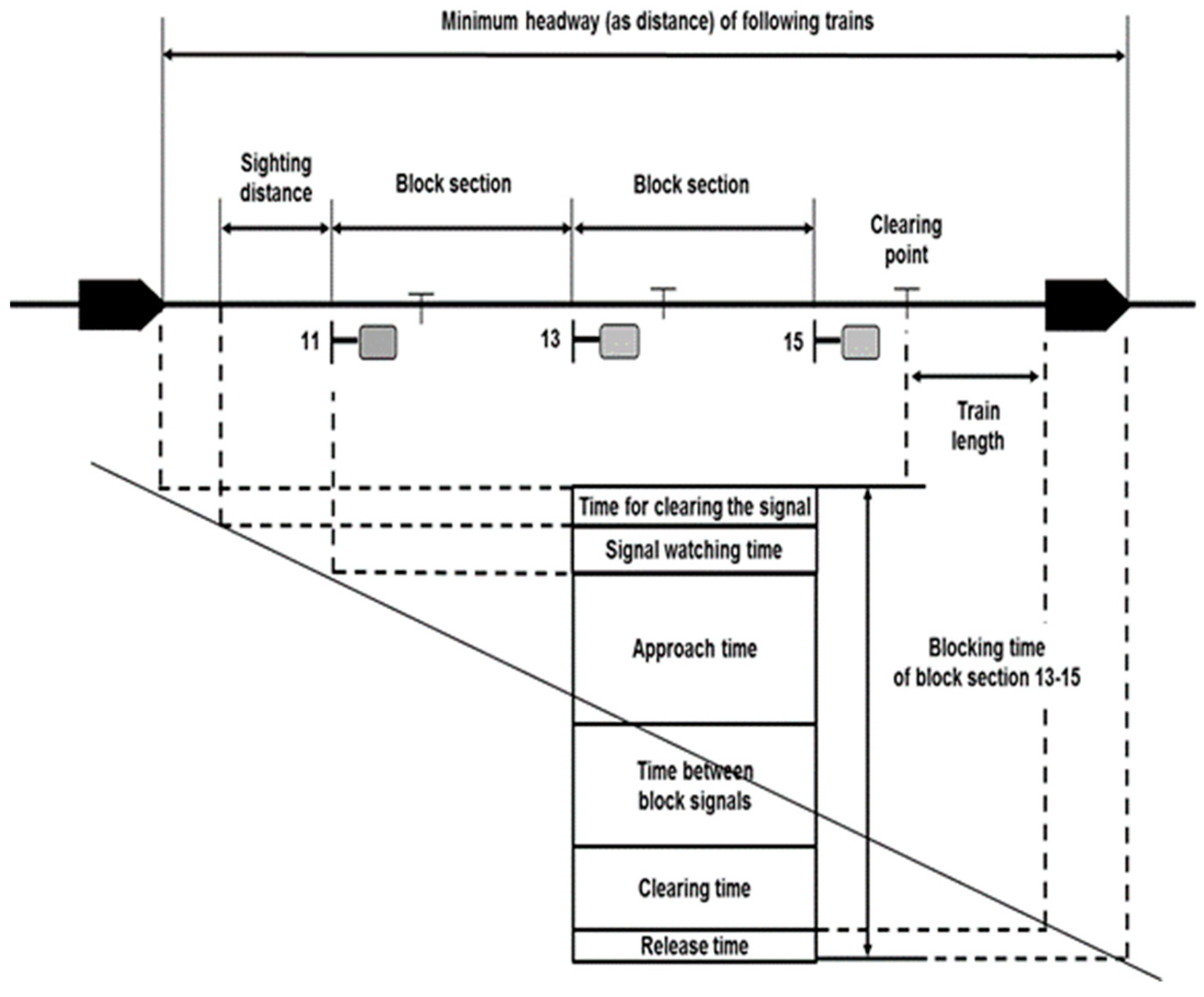
The blocking time between heterogeneous trains must also be considered. Blocking involves setting a boundary at regular distances to prevent the operation of two or more trains simultaneously and to prevent crashes or collisions of trains. To prevent collision between trains, the following trains must start with a specific time interval after the preceding train starts. Figure 4 illustrates the concept of blocking time. The blocking time is the total elapsed time during which a block section is inaccessible to other trains while a train is operating in the black section shown in Figure 4 [27]. The blocking time is completed after the train has completely left the section and all signaling equipment have been reset to their respective normal positions so that another train can be authorized to enter the same section. Therefore, the blocking time of a track section is usually much longer than the time for which the train occupies the section [8,27]. As shown in Figure 4, the blocking time of a block section for a train without a scheduled stop at the entrance of that section consists of the following time intervals in a territory with a fixed block signal system [8,27]:

∙

the time for clearing the signal;

∙

a certain time for the driver to view the clear aspect at the signal in rear that gives the approach indicator to the signal at the entrance of the block section,

∙

the approach time between the signal that provides the approach indicator and the signal at the entrance of the block section;

∙

the time between the block signals, as running time;

∙

the clearing time to clear the block section and–if required- the overlap with the full length of the train; and

∙

the release time to “unlock” the block system.

The minimum headway is a key parameter in selecting the subsidiary tracks that can be used when high-speed trains pass low-speed trains. This study requires subsidiary tracks for high-speed trains to overtake other trains. To analyze the minimum headway between trains, a line with the longest distance between stations is selected from a station with subsidiary tracks from which a low-speed train has started [8]. For the following high-speed train to run at a non-braking speed, the time when the preceding low-speed train arrives at the station with subsidiary tracks and the guaranteed minimum headway to be overtaken by the following high-speed train are required. To meet this condition, the headway (H_w) between the fastest high-speed train (t_hk) and the lowest speed train is required for the low-speed train (t_fk), which is expressed as follows [8]:

$$Hw=\left\{x :x \in ebt{t}_{fk}-bbt{t}_{hk}\right\} for bt=1\cdots n_b$$

(9)

where, ebttfk is the end of the blocking time of the k^th freight train in block section K, bbtthk represents the start of the blocking time of the k^th high-speed train in block section K, and bt is the blocking time.

The objective function of the subsidiary track installation for algorithm modeling is to determine the number of subsidiary tracks. Therefore, this study considers objective functions for determination of subsidiary tracks for overtaking between heterogeneous trains on the same railway track.

$${\displaystyle \sum }_{\forall \in T}(d_n\forall t-a_n\forall t)+{\displaystyle \sum }_{n\in N}{y}_s$$

(10)

where d_n is the departure time at the n^th station, a_n represents the arrival time at the n^th station, and y_s is the extra time that is added to the headway to avoid the transmission of small delays.

3. Algorithm Modeling

3.1. Train Schedule

The date of the train schedule is an array of train types and departure times for respective operations. It has the form of a solution acquired from train scheduling and corresponds to chromosomes in the genetic algorithm. Therefore, the train type and departure time of the train schedule become genes comprising the chromosomes.

The train type is one of the three types: high-speed, passenger, and freight train. The departure time is the time (min) when the train starts from the first station, and the operation start time is set to zero. The train schedule has the following structure: passenger train departing at +1 min, freight train departing at +15 min, a high-speed train departing at +24 min, …, a passenger train departing at +168 min, and a freight train departing at +182 min. Pseudocode is a language that expresses the operating principles of each model when writing programs. It is not written in accordance with the syntax of a specific programming language, but it is a code that writes the algorithm by imitating the code in a universal language. Because pseudocode only imitates a programming language, it cannot be executed in a computer similar to codes written in actual programming languages. It is used to roughly model the algorithm before writing programs in a specific language [29]. Pseudocode is used to express these train schedules, as shown in

Table 2. Pseudo code for train schedule (chromosome).

train schedule = [[passenger train, 1], [freight train, 15], [high-speed train, 24]… [passenger train, 168], [freight train, 182]]

.

When the calculation progresses, the evacuation and delay data can be added to each train operation.

3.2. Scheduled Waiting Time

The scheduled waiting time data contain the array of the train type for which evacuation is generated, the departure time of the train for which evacuation is generated, the station where the subsidiary track for evacuation is located. The scheduled waiting time is zero when the train departing at a different time passes during the stopping at the stopping station. However, the evacuation and scheduled waiting time data are also added in this case because the subsidiary track is required. The evacuation and scheduled waiting time data become the standard for evaluating the fitness of the genetic algorithm, and the place of the required subsidiary track can be checked in the corresponding train schedule.

The delay data have the structure of an 8-min delayed departure at the second station due to a passenger train departing at +29 min, a 12-min delayed departure at the second station due to a freight train departing at +42 min, and a zero-min delayed departure from the fourth station due to a high-speed train departing at +75 min. The pseudocode is shown in

Table 3. Pseudocode for scheduled waiting time.

scheduled waiting time = [[29, passenger train, 1, 8], [42, freight train, 1, 12], …, [75, high-speed train, 3, 0]]

. In addition,

Table 4. Pseudocode for train schedule and scheduled waiting time.

train schedule = [ [ passenger train, 1, [1, 17, 54, … 185], [[29, passenger train, 1, 8], [42, freight train, 1, 12], [75, high-speed train, 3, 0], …] ], … ]

shows the train operation schedule structures and the scheduled waiting times.

3.3. Station Data

The station data contain an array of the movement time from the previous station to the present station and whether each type of train stops at the station. The station data form the basic data for various train operations, such as calculating the train schedule. The departing station is excluded because it does not have a preceding station, and whether or not the trains have stopped is meaningless. Whether the train has stopped at the last station is also not considered here. The structure of the station data is as follows:

• Movement time from the first to the second station: passenger train, 7 min; high-speed train, 15 min; and freight train, 23 min.
• Stopping order at the second station: a passenger train does not stop at the second station, a high-speed train stops, and a freight train does not stop.
• Movement time from the second to the third station: passenger train, 14 min; high-speed train, 20 min; and freight train, 38 min. Stopping order at the third station: a passenger train stops at the third station, a high-speed train stops, and a freight train does not stop.
• Movement time from the sixth to the last station: passenger train, 19 min; high-speed train, 25 min; and freight train 47 min.

The pseudocode is shown in

Table 5. Pseudocode for station data.

station = [[7, 15, 23, false, true, false], [14, 20, 38, true, true, false],…, [19,25,47]]

.

3.4. Structure of Genetic Algorithm

The genetic algorithm applied to the subsidiary track search process is given in Figure 5.

The initial population involves the number of chromosomes produced. Here, a population means a set of chromosomes, and a chromosome is considered to be a train schedule. A chromosome consists of genes, and a gene is considered to be a train. An array of departure times that retains the passenger train and freight train is generated to create a chromosome (train schedule) that meets the above conditions. While generating the chromosome, a train schedule that considers the location of subsidiary tracks is created sequentially in accordance with the gene sequence. After this process, the fitness of this chromosome is evaluated. If the constraint condition is not satisfied, the algorithm moves on to the selection stage. During selection, the chromosomes are haphazardly chosen, and the chromosome that has high requirements of subsidiary tracks is excluded from the next generation. The chromosomes that remain after selection alter the surpassing genetic qualities via crossover. Then, the genes of the chromosomes are moved to other location to obtain diverse solutions at the mutation. Improper chromosomes after mutation are changed to qualified chromosomes after repair. If the condition is satisfied, the algorithm is completed. The pseudocode for an array of departure time for the passenger and freight train is shown in

Table 6. Pseudocode for an array of departure time for the passenger train [6]

list of departure times for passenger trains = []; generate a list of departure times for passenger trains = function() { first passenger train departure time = passenger train expected interval/2; for (i = First passenger train departure time; i <= calculation time; i += passenger train expected interval) { list of departure times for passenger trains.push(i);   } };

and

Table 7. Pseudocode for an array of departure time for the freight train [6].

Add freight train schedule = function(train schedule) { for (i = 0; i < number of freight trains; i ++) { list of addable train count and departure times = Check if freight trains can be added (train schedule); if (addable train count < freight train count) { exception(); break; }

.

After generating chromosome (train schedule) with initial population, each chromosome (train schedule) is considered for fitness. The fitness is represented by the location of subsidiary track that is generated by heterogeneous trains operated in same railway track when producing the chromosome (train schedule). Analyzing when the scheduled waiting time occurs can help find the location of the subsidiary track in chromosomes (train schedules in

Table 8. Pseudocode for calculating the fitness [6].

scheduled waiting time of general train = 0; scheduled waiting time of freight train = 0; for(train schedule) { if (general train) { scheduled waiting time of general train += general train arrival time − general train departure time − running time of general train without delay; } if (freight train) { scheduled waiting time of freight train += freight train arrival time − freight train departure time − running time of freight train without delay; } };

).

If the solution is not found after the fitness calculation, a new population is created based on the fitness of the current population. For a new population, select two chromosomes (train schedule) from the current population, cross genes (trains) to generate new chromosomes, induce mutation with a certain probability to obtain a diversity of solutions, and determine whether the newly-created train schedule is fit. If not, then repair it. After the new population is created, the fitness evaluation is performed again. The pseudocodes for the fitness calculation, the selection, the crosover, the mutation and the repair are represented in

Table 9. Pseudocode for selection [6].

for(order; population) { population [order].start roulette wheel area = (order == 0) ? 0 : population[order - 1].stop roulette wheel area − 1; population[order].stop roulette wheel area = best fitness * 4 − (best fitness * 2 * (population[order].fitness - best fitness) / (maximum fitness – best fitness) + best fitness); } random number 1 = generate random number(0, population[last].stop roulette wheel area); random number 2 = generate random number(0, population[last].stop roulette wheel area);

,

Table 10. Pseudocode for crossover [6].

new chromosome = [[]; chromosome 1 = sort by train type (chromosome 1); chromosome 2 = sort by train type (chromosome 2); for(order; chromosome 1) { random number = generate random number(0, 1); if (random number < 0.5) new chromosome.push (chromosome 1[order]); else new chromosome.push (chromosome 2[order]); }

,

Table 11. Pseudocode for mutation [6].

Random number = generate random number(0, 1000); if (random number <= 15) { random number = generate random number(0, chromosome length − 1); chromosome[random number] = get a new departure time (); }

and

Table 12. Pseudocode for repair [6].

for(order; train schedule) { train schedule[order] = calculation of detailed operation schedule(train schedule[order]); if(!train schedule[order].fitness) { train schedule.delete(order); train schedule[order] = get a new departure time (); } }

.

4. Simulation Results and Discussion

4.1. Conditions and Scenarios

To simulate the algorithm presented in Section 3, the input and output data are based on the hypertext markup language 5 (HTML5) and Javascript/jQuery algorithms. These algorithms were first used for research purposes but were then implemented to allow user interface modification for universal utilization. The railroad track is set with a 60-km length with seven stations in total. This includes the terminal and the intermediate stations and 10-km straight track sections, with no curves between each station, as shown in Figure 5. It is assumed that on the considered railroad track, the high-speed train stops for 2 min at the fourth station, the passenger train stops for 1 min at every station, and the freight train passes through every station. According to an actual train operation timetable, the stopping time of high-speed trains is 2 min and that of passenger trains is 1 min. The high-speed train plays the role of an express railway, and the passenger train plays the role of a slow train. However, freight trains stop at stations for a long time for movement of freight in most cases, and the criteria for this stopping time differ by freight amount, type, and station size. Hence, in this study, we assumed that the freight trains pass through all stations. The high-speed train and passenger train are given random train schedules that satisfy the genetic algorithm considered in this study, and the departure time of the freight train is calculated after the schedules of the high-speed train and passenger train are calculated.

The simulation was performed 100 times for each case on the railroad track in Figure 6, as shown in

Table 13. Train operation frequencies in different simulation cases.

Division	The Train Operation Frequency According to Cases
	Case 1	Case 2	Case 3	Case 4	Case 5	Case 6
High-speed train	3	3	6	6	9	9
Passenger train	6	9	9	3	3	6
Freight train	9	6	3	9	6	3

. The numbers of subsidiary tracks were determined when heterogeneous trains were operated on the same track with variations in the scheduled waiting time. The number of stations that need a subsidiary track are calculated on the assumption that all intermediate stations can be overtaking and evacuation. In this study, the operation times for each train type, for 3 h, were set to 3 min for a high-speed train, 5 min for a passenger train, and 7 min for a freight train. The velocities of each train type between stations (Figure 6) were set to 200 km/h for a high-speed train, 120 km/h for a passenger train, and 85.7 km/h for a freight train.

Thus, the purpose of the simulation was to analyze the location of the subsidiary tracks due to overtaking and evacuation when different types of trains are operating on one route. When each train was operated on the railway track shown in Figure 6, a total of six cases were analyzed according to different train operation frequencies, as shown in Table 13. Each train had a different running time between stations, as shown in Figure 6. Each case is defined as follows.

Case 1: The train operation frequency for each train type is three for a high-speed train, six for a passenger train, and nine for a freight train.

Case 2: The train operation frequency for each train type is three for a high-speed train, nine for a passenger train, and six for a freight train

Case 3: The train operation frequency for each train type is six for a high-speed train, nine for a passenger train, and three for a freight train.

Case 4: The train operation frequency for each train type is six for a high-speed train, three for a passenger train, and nine for a freight train.

Case 5: The train operation frequency for each train type is nine for a high-speed train, three for a passenger train, and six for a freight train.

Case 6: The train operation frequency for each train type is nine for a high-speed train, six for a passenger train, and three for a freight train.

4.2. Analysis and Discussion of Simulation Results

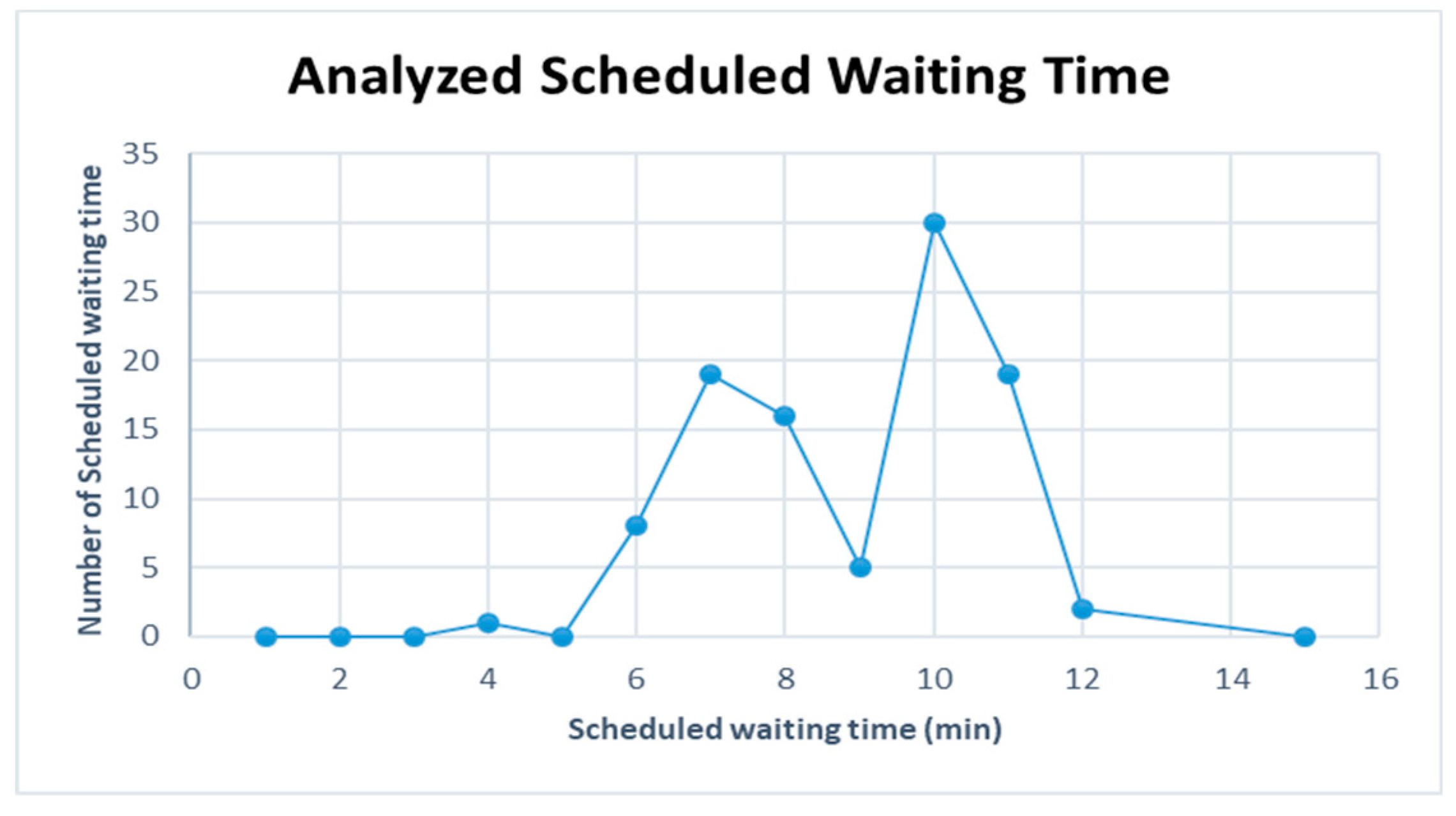
The scheduled waiting times according to the three types of train operation frequency are analyzed, assuming that all the intermediate stations of the considered railroad tracks (Stations 2–6) have a subsidiary track.

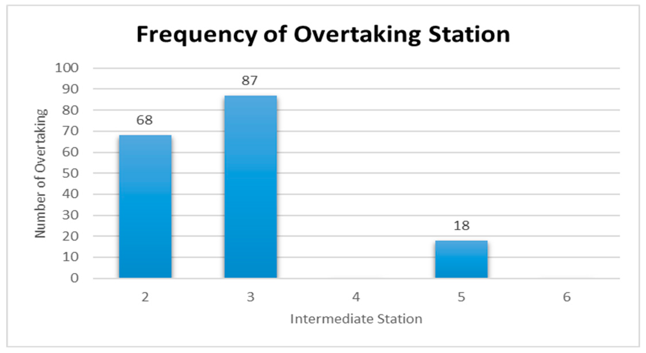
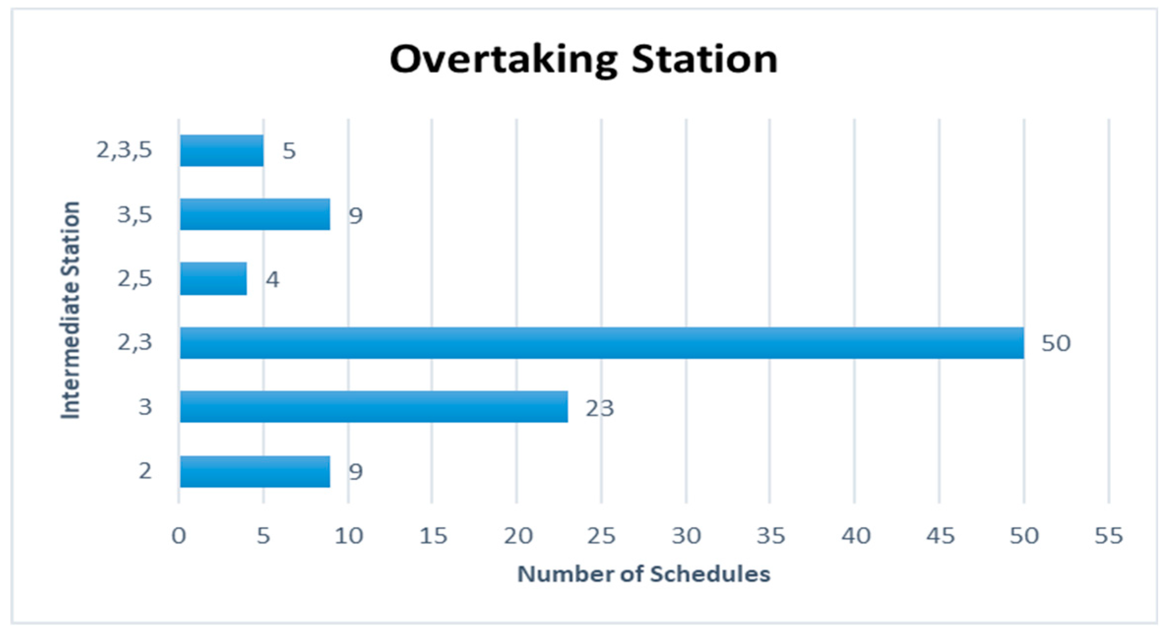
Figure 7, Figure 8 and Figure 9 are represented for the schduled waiting time, the frequency of overtaking station and number of train scheules for overtaking in Case 1. In Case 1, the scheduled waiting time of 10 min showed the highest frequency of 30 times in 100 simulations. In all the analyzed train schedules, the passenger train and high-speed train overtook the freight train and overtaking occurred 87 times at Intermediate Station 3, 67 times at Intermediate Station 2, and 18 times at intermediate station 5. Intermediate stations 2 and 3 required subsidiary tracks because overtaking occurred at these stations in 50 of the total 100 time schedules.

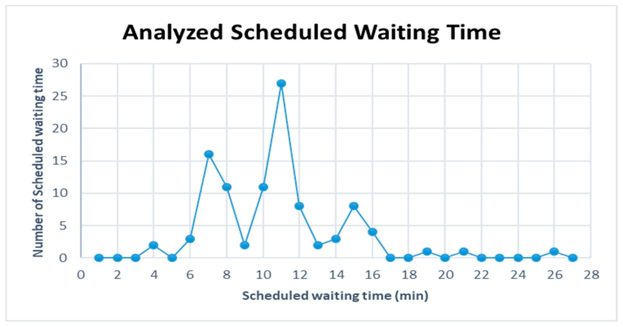
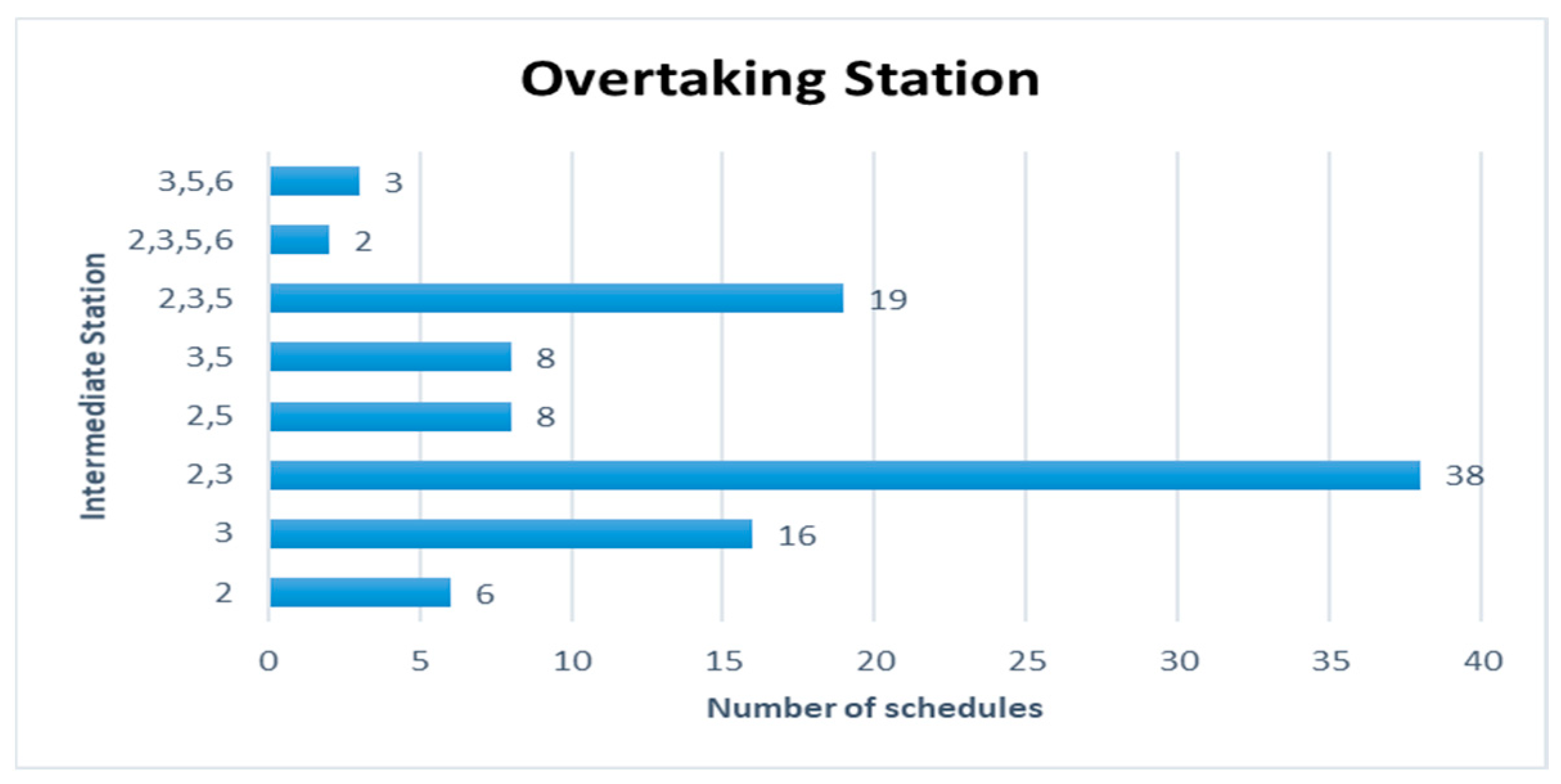
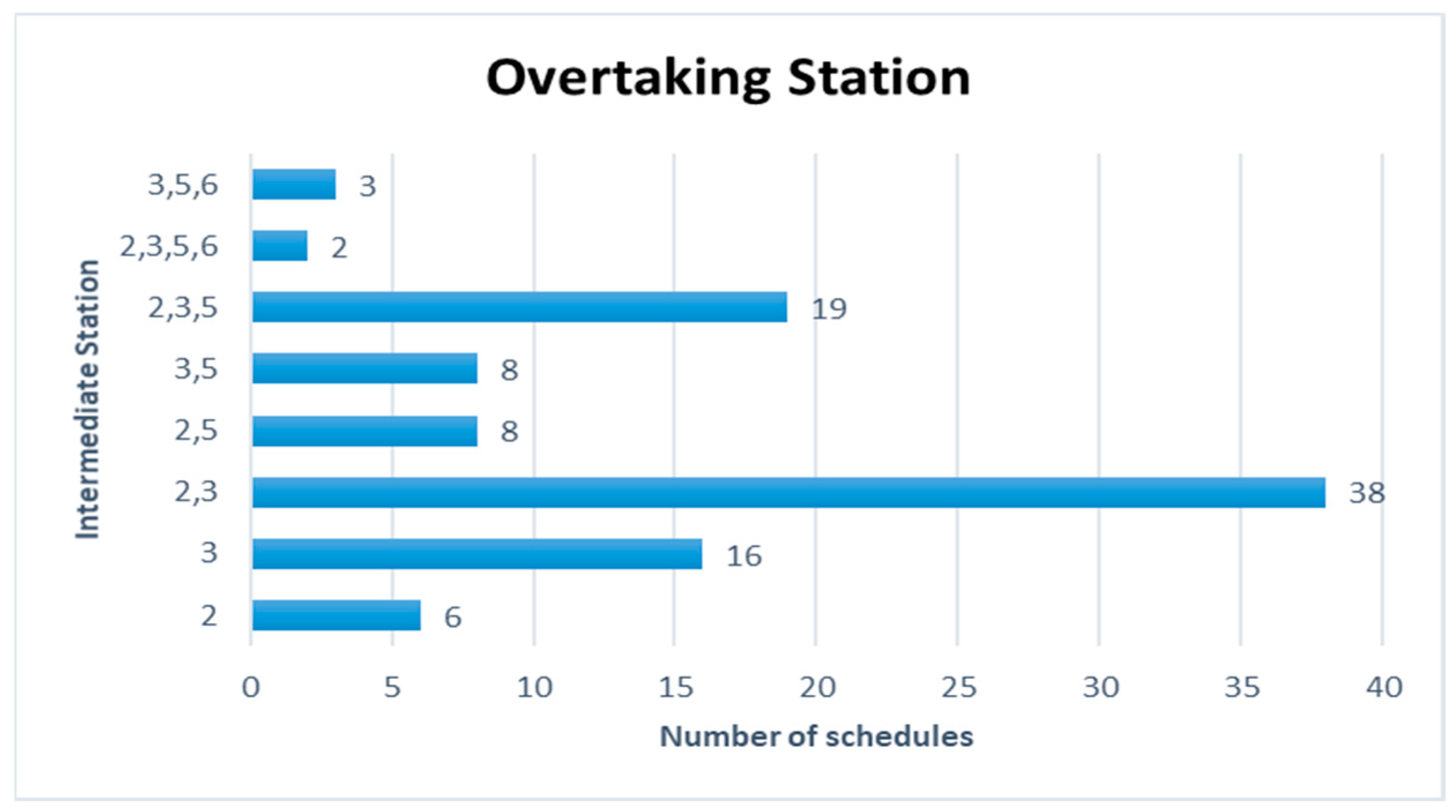
Figure 10, Figure 11 and Figure 12 are represented for the schduled waiting time, the frequency of overtaking station and number of train scheules for overtaking in Case 2. In Case 2, the scheduled waiting time of 11 min showed the highest frequency of 27 times in 100 simulations. In all the analyzed train schedules, the passenger train and high-speed train overtook the freight train as in Case 1, and the overtaking occurred 86 times at Intermediate Station 3, 73 times at Intermediate Station 2, and 40 times at Intermediate Station 5. This shows that the number of passenger and high-speed trains overtaking the freight train at Intermediate Stations 2 and 5 is larger than in Case 1. This is because the number of passenger trains is larger and the number of freight trains is smaller than those in Case 1, resulting in more passenger trains overtaking the freight trains. Intermediate Stations 2, 3, and 5 required subsidiary tracks because overtaking occurred at Intermediate Stations 2 and 3 in 38 time schedules and Intermediate Stations 2, 3, and 5 in 19 time schedules out of the 100 analyzed time schedules. The number of train schedules in which overtaking occurred only at Intermediate Station 3 was 16.

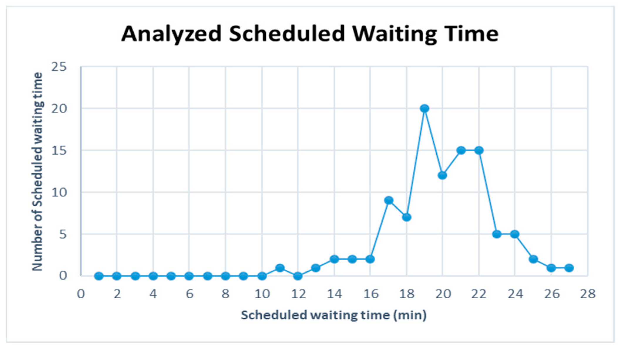
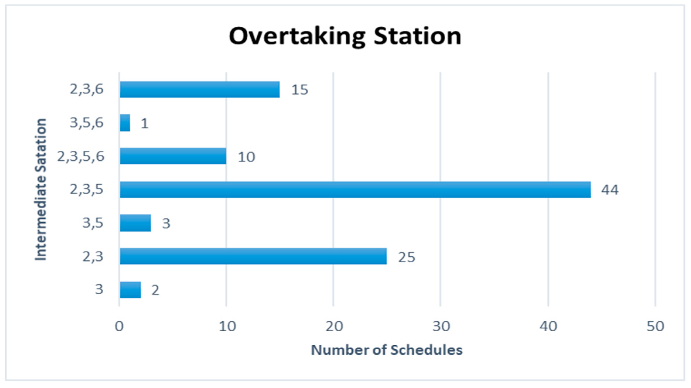
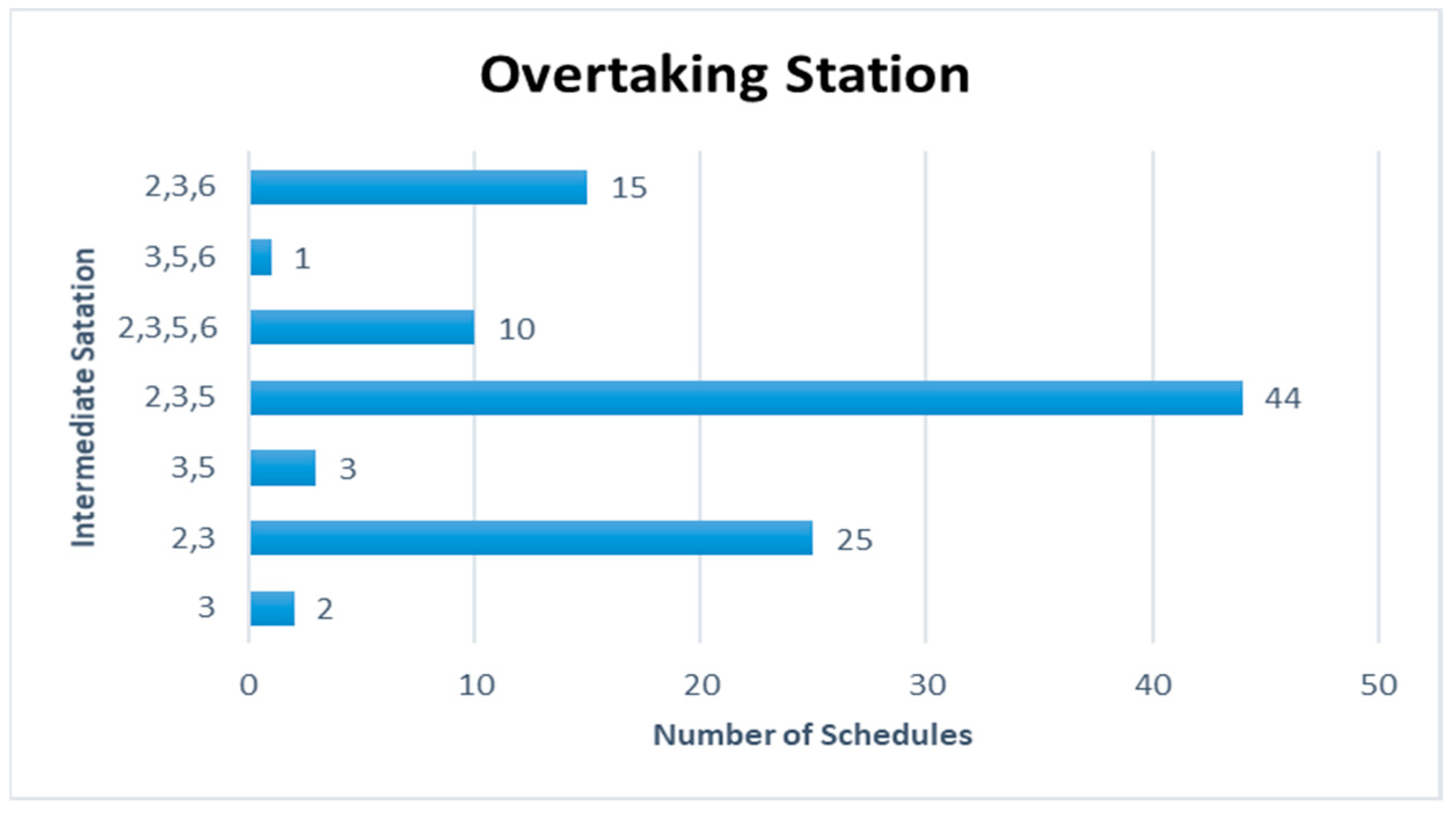
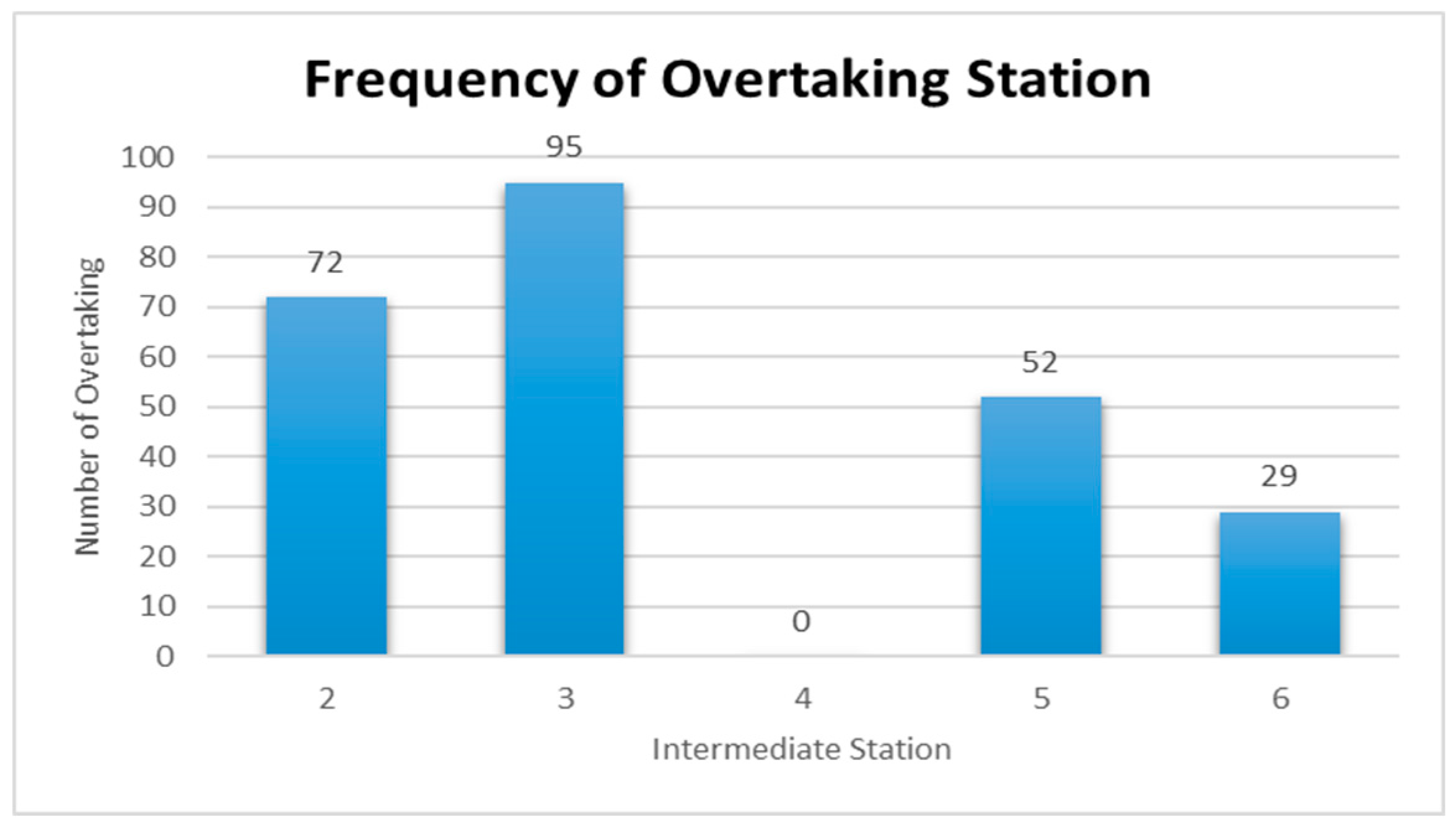
Figure 13, Figure 14 and Figure 15 are represented for the schduled waiting time, the frequency of overtaking station and number of train scheules for overtaking in Case 3. In Case 3, the scheduled waiting time of 19 min showed the highest frequency of 20 times in 100 simulations, followed by the scheduled waiting times of 21 and 22 min with 15 times. In all the analyzed train schedules, the passenger train and high-speed train overtook the freight train, as in Cases 1 and 2. Overtaking occurred in all simulations at Intermediate Station 3, and 94 times at Intermediate Station 2. The overtaking frequency increased because, even though the operation frequency of passenger trains is small in Case 3, the two trains with high-speed differences, the high-speed train, and freight train, were operated 6 and 9 times, respectively. Out of the 100 analyzed train schedules, overtaking occurred at Intermediate Stations 2, 3, and 5 in 44 time schedules and at Intermediate Stations 2 and 3 in 25 time schedules.

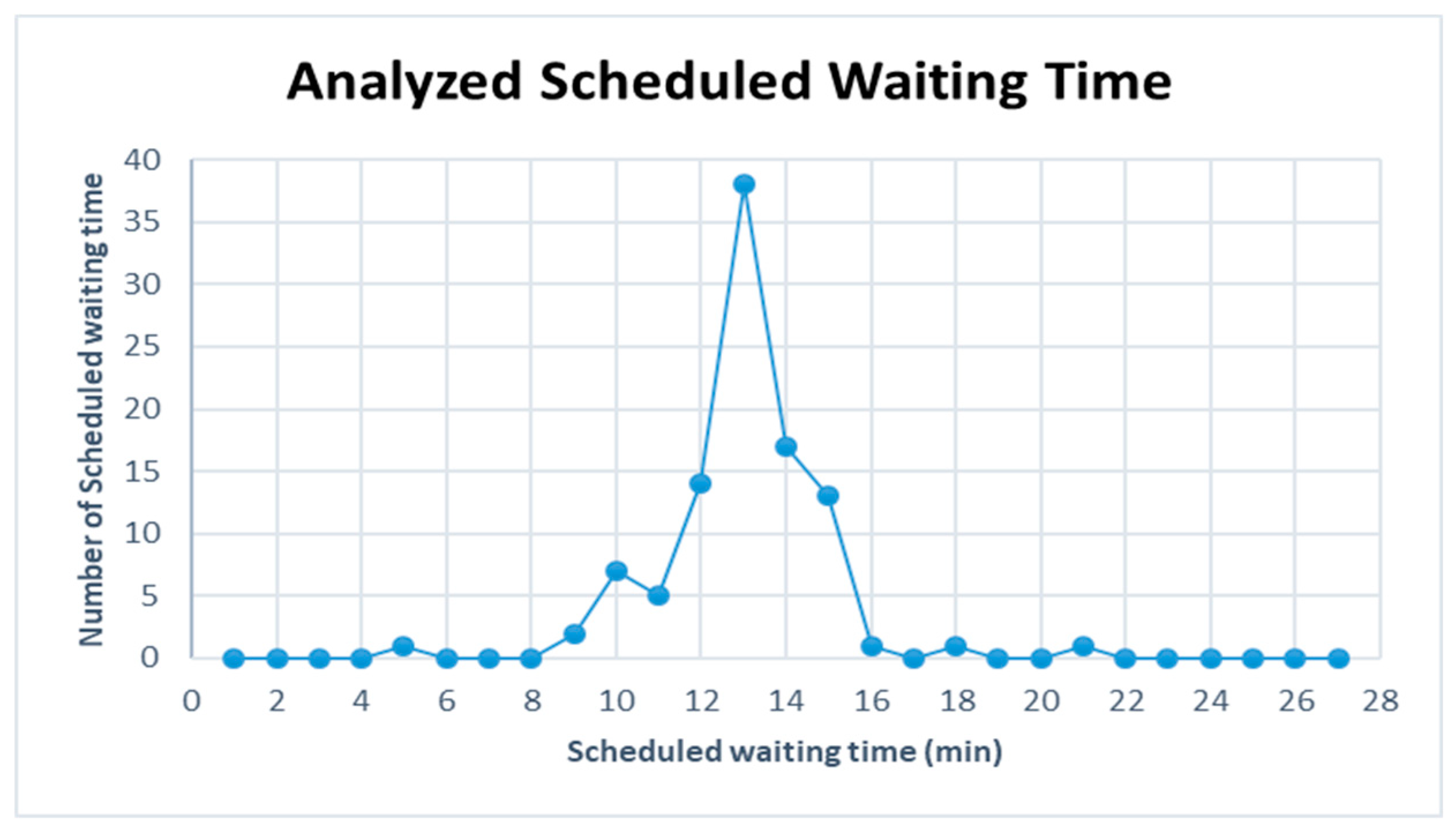
Figure 16, Figure 17 and Figure 18 are represented for the schduled waiting time, the frequency of overtaking station and number of train scheules for overtaking in Case 4. In Case 4, the scheduled waiting time of 13 min showed the highest frequency of 38 times in 100 simulations. The passenger train and freight train were overtaken by the high-speed train in 99 time schedules, except for 1 train schedule. This is because the operation frequencies of the high-speed train and passenger train are 6 and 9, respectively, and the freight trains are overtaken by a passenger train and high-speed train. Overtaking occurred 95 times at Intermediate Station 3, and 72 times at Intermediate Station 2. Out of the 100 analyzed train schedules, overtaking occurred at Intermediate Stations 2, 3, and 5 in 28 train schedules, and at Intermediate Stations 2 and 3 in 19 time schedules.

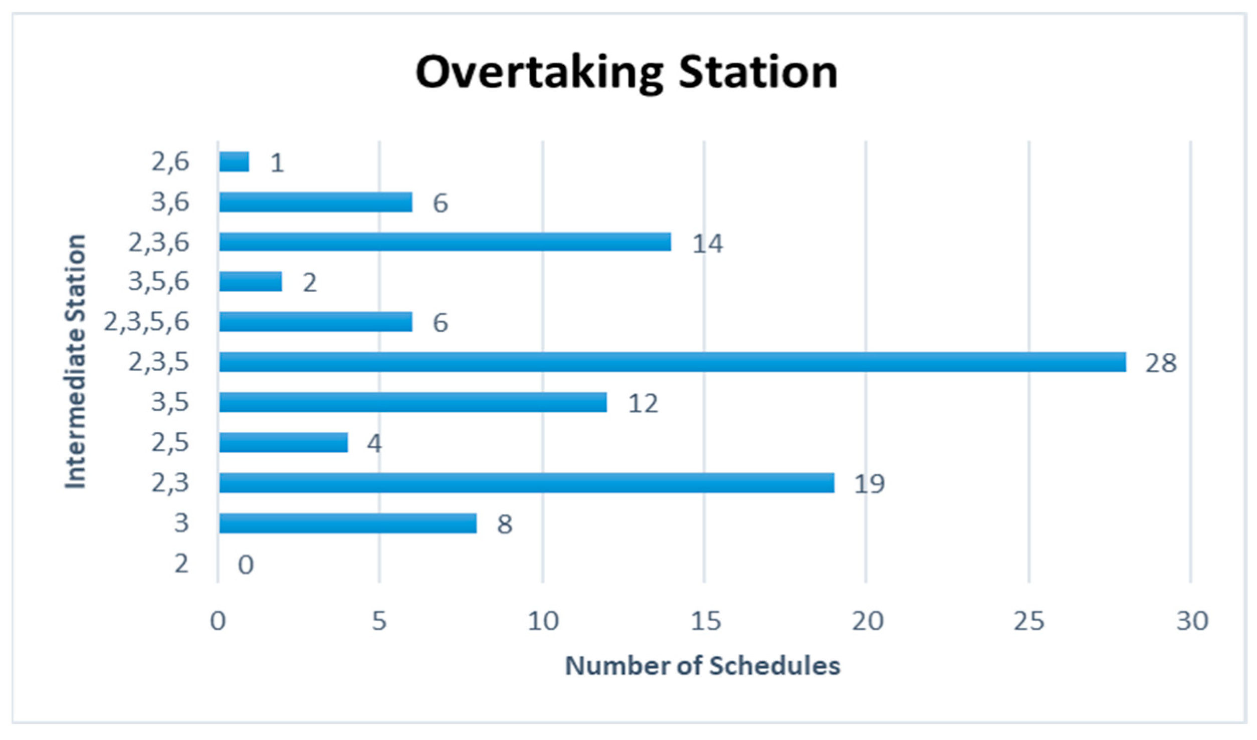
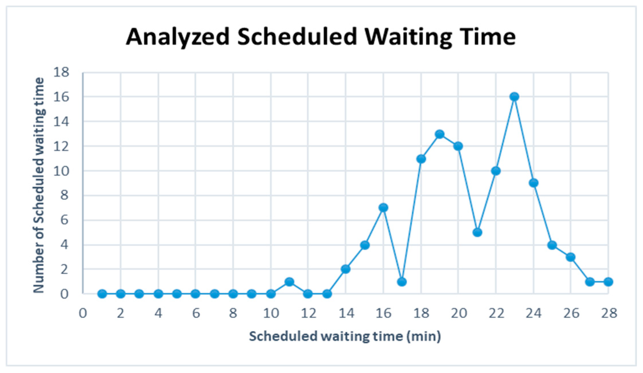
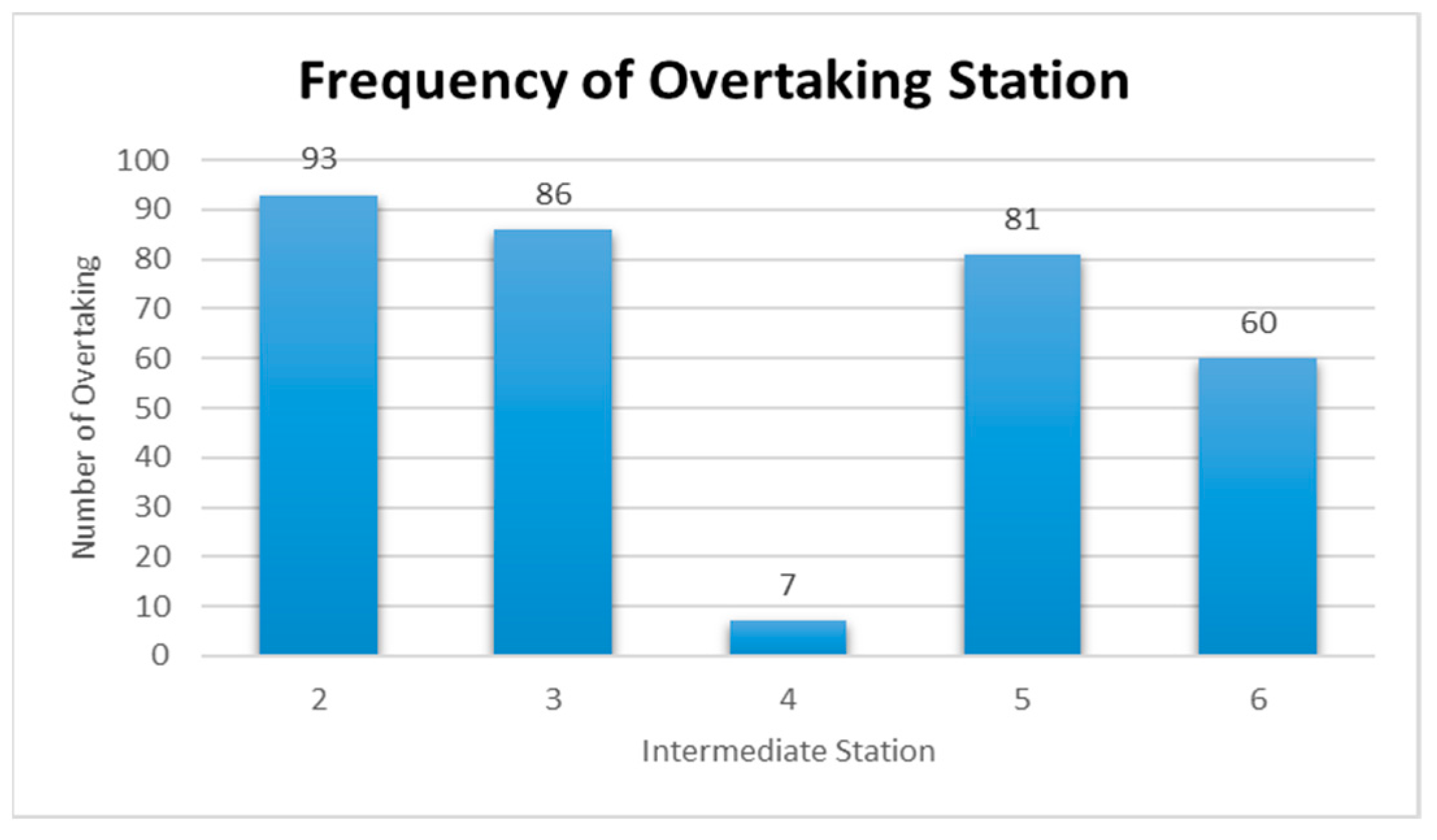
Figure 19, Figure 20 and Figure 21 are represented for the schduled waiting time, the frequency of overtaking station and number of train scheules for overtaking in Case 5. In Case 5, the scheduled waiting time of 23 min showed the highest frequency of 16 times in 100 simulations, followed by 21 and 22 min of scheduled waiting time with 15 times. In all the analyzed train schedules, the passenger train and high-speed train overtook the freight train. This is because the operation frequency of the passenger train is small (3 times), whereas the operation frequency of the high-speed train is the highest (9 times). Overtaking occurred 93 times at Intermediate Station 2, 86 times at Intermediate Station 3, and 81 times at Intermediate Station 5. Out of the 100 analyzed train schedules, overtaking occurred at Intermediate Stations 2, 3, 5, and 6 in 31 train schedules and at Intermediate Station 2, 3, and 5 in 30 train schedules.

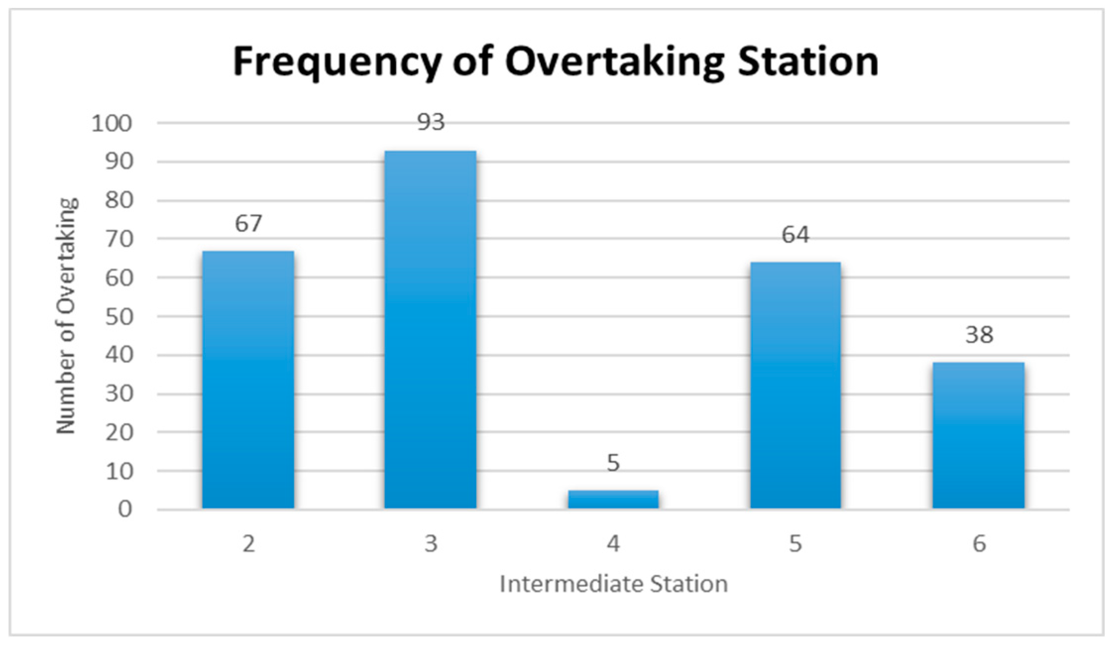
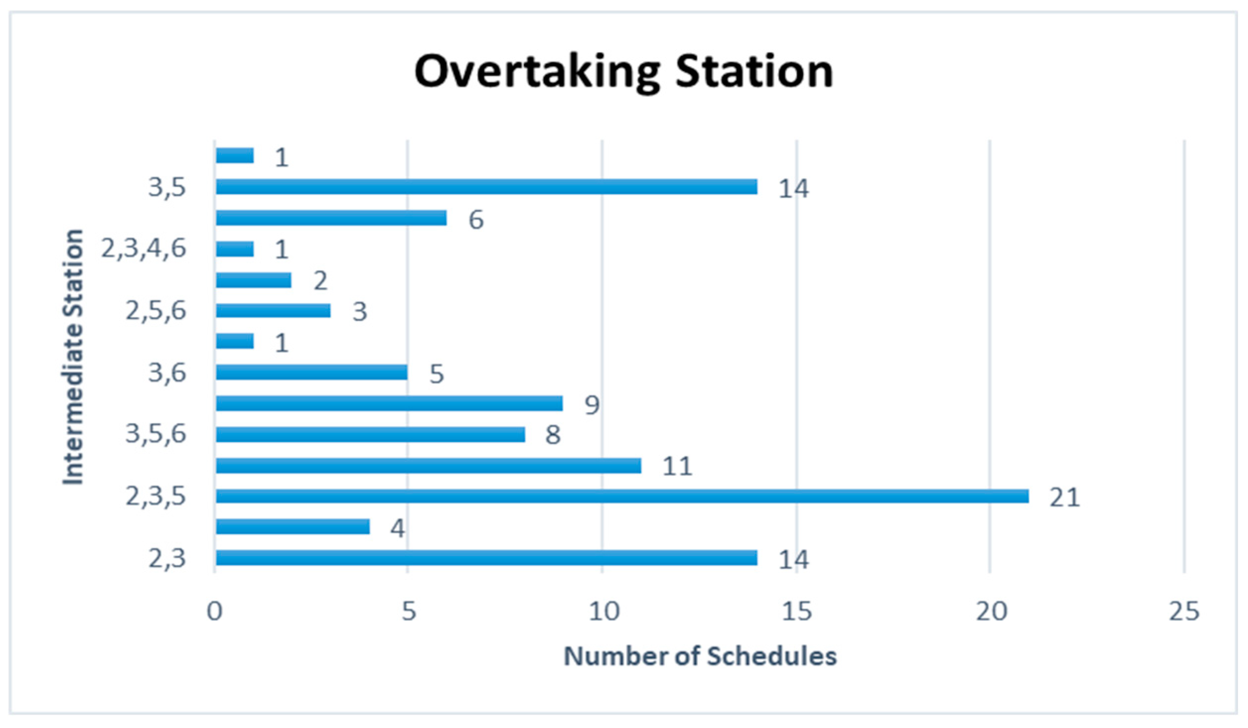
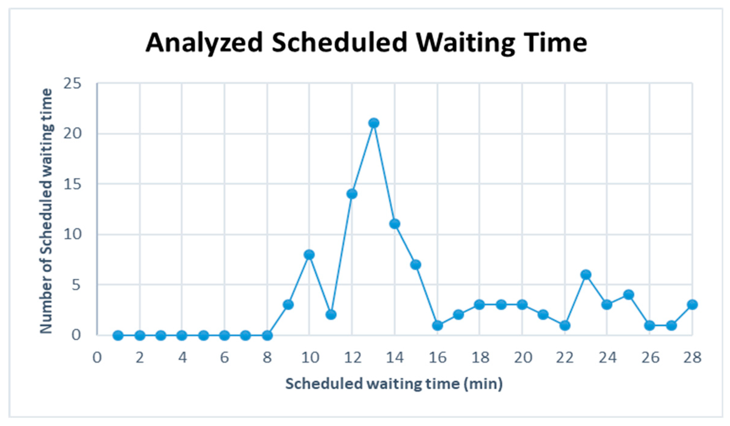
Figure 22, Figure 23 and Figure 24 are represented for the schduled waiting time, the frequency of overtaking station and number of train scheules for overtaking in Case 6. In Case 6, the scheduled waiting time of 13 min showed the highest frequency of 21 times in 100 simulations, followed by the scheduled waiting time of 12 min with 14 times and the scheduled waiting time of 14 min with 11 times. In all the analyzed train schedules, the passenger train and freight train were overtaken by the high-speed train. Overtaking occurred 93 times at Intermediate Station 3, 67 times at Intermediate Station 2, and 64 times at Intermediate Station 3. Of the 100 analyzed train schedules, overtaking occurred at Intermediate Stations 2, 3, and 5 in 21 train schedules and Intermediate Stations 2 and 3 in 14 train schedules.

Table 14. Frequency of overtaking station for each case.

Division	Number of Trains			Frequency of Overtaking Station					Total
	High-Speed Train	Passenger Train	Freight Train	Intermediate Station 2	Intermediate Station 3	Intermediate Station 4	Intermediate Station 5	Intermediate Station 6
Case 1	3	6	9	68	87	0	18	0	173
Case 2	3	9	6	73	86	0	40	5	204
Case 3	6	3	9	94	100	0	56	28	278
Case 4	6	9	3	72	95	0	52	29	248
Case 5	9	3	6	93	86	7	81	60	327
Case 6	9	6	3	67	93	5	64	38	267

summarizes the frequency of overtaking for each case. The overtaking frequency was the highest at Intermediate Station 3 in all cases except Case 5. This leads to the conclusion that Intermediate Station 3 requires a subsidiary track even though the operating frequency of each train on the considered track differs. Intermediate Station 4 showed a significantly low overtaking frequency because it is a station where the high-speed train and passenger train stop. In Case 5, the largest number of overtaking, 327 times, occurred when the operation frequencies of the high-speed train and freight train were 9 and 6, respectively. This shows that the number of overtaking increases if the operating frequency of a high-speed train is higher than that of a freight train. For Case 3, where the operating frequencies of the high-speed train and freight train, the two trains with the highest speed difference, are high at 9 and 6, respectively.

5. Conclusions

In this study, the scheduled waiting times were calculated according to the operating frequencies of a passenger train, high-speed train, and freight train when the trains are operated on the same track. In addition, the positions of the subsidiary tracks were stochastically analyzed, and their effects on the train operation service were investigated using a metaheuristic algorithm. While previous studies have solved the NP-hard problem mainly using heuristic methods, we used a genetic approach to enhance the reliability of the mathematical model. The model was used to determine stations that need subsidiary tracks for overtaking trains in the strategic and tactical steps of the railway planning procedure. The waiting time function, the guaranteed headway for high and low-speed trains at a station, the blocking time and the minimum headway were considered as the constrain conditions in this research. Polynomials for the constraint conditions were mentioned and differences for each train such as operation frequency, duel time, velocity, stopping station were regarded as the constrain conditions when doing simulation.

This was done with different operation speeds and stopping stations for each train in the test track with the same distances between stations for each case. This study was performed to determine the requirement of a subsidiary track when operating heterogeneous trains on the same railroad, and the model can be applied universally if it is upgraded.

In general, the shortest scheduled waiting time can be considered to be the best train schedule, but the present study aimed to select the subsidiary track according to the operating frequencies of heterogeneous trains. The results showed that intermediate station 3 requires a subsidiary track because of the high occurrence of overtaking. Further research on the analysis of the optimal train schedule and the calculation of track capacity according to the scheduled waiting time is required. In addition, the effects of the distance between stations or the speed difference between heterogeneous trains on the selection of the position of a subsidiary track need to be analyzed. The ultimate objective of this study was to increase the objectivity and reliability of the model by determining the location of the main station using an analytical method rather than determining the location of the main station based on the railway planner’s experience. To increase the objectivity and reliability, it is necessary to study various railway environments. Although the distance between stations is the same in this study, the actual railway route is composed of various distances between stations. As a result, the speed and driving time of the trains considered vary. In addition, it is necessary to apply the number of times of operation of each train based on transportation demand during actual operation. In future studies, objective and practical railway planning could be achieved during railway construction using our proposed model. Furthermore, achievements in the field of railway planning will be attained through follow-up studies.