1. Introduction
The increasing trend in energy demand over the world is intimately related to the rise in the quality of life and human needs. The three main energy consumers are the transportation sector, industry and the tertiary sector (housing and services) [
1]. As the main objective is to reduce energy consumption by using it in a rational way, many activities are focused on optimizing the performance of energy systems. That said, the residential and commercial buildings still account for 20–40% of the total energy consumption in developed countries and its tendency has been increasing year by year.
Buildings consume energy throughout their entire life cycle, starting from the construction until they are demolished [
2]. Nevertheless, a great amount of energy consumption takes place during the operational period, in order to satisfy the demand of heating, domestic hot water (DHW), ventilation and air conditioning (HVAC) to provide indoor comfort conditions. An overview of building energy consumption is given in reference [
3] which is mainly focus on the status and current trends on energy use in buildings in Madagascar.
1.1. Exergy and Buildings
To achieve the energy-saving goal, it is very helpful to include exergy methods in the analysis of buildings, both for the building envelope and for the facilities; as done in reference [
4] where the methods and the metrics of the exergy analysis in buildings are described. Above all, the recent published book of reference [
5] can be considered one of the most complete works connected with exergy analysis and thermoeconomics of buildings in which all the issues related to design and exergy application in buildings is deeply explained.
In order to introduce the exergy concept in buildings it is necessary to review the way in which energy is transformed from one form to another. According to the first law of thermodynamics, energy is always conserved in all processes i.e., heat can be obtained from combustion of a fuel or from an electrical source, etc. and always the quantity of energy contained in the fuel or the electrical energy is the same as the heat flux obtained [
6]. However, all the energy conversions take place in a definite direction i.e., in the transformation of heat into work a part of the heat flux has to be transferred to a cold source, as a heat loss, and cannot be recovered.
Moreover, if a system undergoes a reversible process, both the system and its surroundings can always be restored to their original state. It is obvious that no process is reversible and because of those irreversibilities the energy quality degrades. Indeed, this is described by the second law of thermodynamics.
The quality of the energy, which is precisely what exergy reflects, is its capacity to be transformed into useful work. Depending on its nature, some energy forms can be entirely converted into useful work, such us electricity or any form of mechanical energy, while other energy forms, as heat or thermal energy, are only partially able to be converted into work [
7]. Hence, electricity is 100% exergy and only a small part of a heat flux is exergy. Consequently, when the capacity of producing useful work is reduced, exergy is being destroyed. This is related to imperfections in the processes, which are called irreversibilities.
Therefore, exergy allows analysis of processes and detection of real imperfections. Then, the exergy method can be implemented for design and optimization purposes, particularly in buildings. As an example, in reference [
8] an exergetic methodology to promote improvements in buildings’ thermal systems is explained. Accordingly, exergy application is especially interesting in buildings because different quality levels of energy [
9] are mixed together to cover the energy demands. For example, on the one hand, electricity is consumed for lighting and electrical appliances. On the other hand, other forms of high-quality energy, such as natural gas, are usually consumed for heating or cooling purposes. It is worth noting that thermal comfort is acquired by tempering the indoor air a few degrees above or below the ambient temperature, so low-quality energy would be enough to cover such demands. Therefore, if a high-quality resource is used for indoor conditioning, there is a mismatch in energy qualities. As a result, significant exergy destruction occurs which is much greater than heat losses accounted for through a first law balance.
Therefore, exergy methods represent more faithfully the energy conversion processes than common energy methods, which can erroneously quantify the real losses of a system. Besides, as justified in reference [
10], comparison among renewable and non-renewable energy building systems can be more fairly done under this perspective. Therefore, referring to the building sector, a great potential still exists to enhance the matching between the quality of energy sources and their final destination, in order to avoid irreversibilities and achieve as a result the decrease of costs.
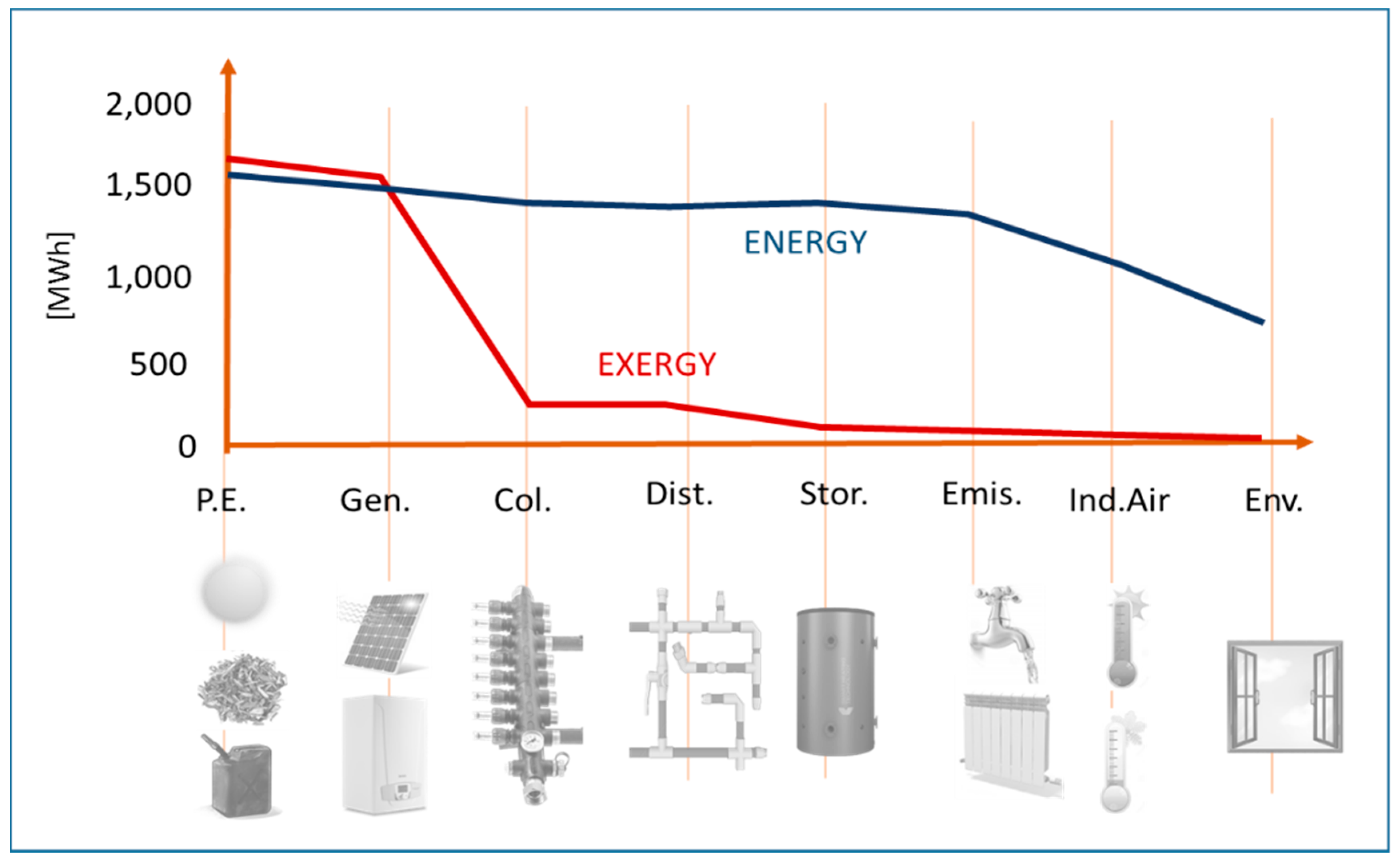
Figure 1 shows, as an example, the annual energy and exergy flows of a building’s heating and DHW facility located in a moderate climate of the Basque Country (northern Spain); this example is taken from reference [
11]. The graph is divided into the different parts of the energy chain: from primary energy (P.E.: fossil fuels, renewables sources, etc.), generation (Gen.: engines such as boilers, solar collectors, etc.), collectors (Col.: gathering of produced heat, etc.), distribution (Dist.: pipes, distribution valves, etc.), storage (Stor.: inertial tanks, seasonal storages, etc.), terminal elements (Emis.: taps, heaters, fan coils etc.) and finally to the indoor air (R.A.: area to temperate) and the environment (Env.: outside). The significant differences in the values of both flows are apparent.
1.2. Exergy and Thermoeconomics
According to its definition, exergy can be considered as a rational parameter to assign costs along an energy system. Engineers and architects work to solve design problems and to optimize buildings under energy, economic and environmental perspective. If exergy analysis is connected to economics, a cost allocation procedure can be developed which becomes a powerful tool for systematically analyzing thermal systems.
The economic analysis in building thermal installations aims to calculate the cost of all flows and particularly of final flows (heating, cooling and DHW) from the prices of the fuels consumed and the investment and maintenance costs of equipment. However, this information is not enough to calculate the costs when the system has several products, as we need guidance for allocating these costs among the different products. Thermodynamic analysis allows calculation of the efficiency of each process, as well as location of the irreversibilities, but it cannot evaluate the effect of irreversibility throughout the production process in terms of costs [
8].
The knowledge area that gathers exergy analysis and economics is known as Thermoeconomics, although the most appropriate name is Exergoeconomics, as it was proposed in 1984 by Tsatsaronis [
12]. Referring to that author, the so-called advanced exergy analysis methodology has been developed and, in recent years, some application in buildings systems emerged, such as Refs. [
13,
14]. The work done in those references aim to solve the problems related to dynamic conditions in buildings.
As mentioned, the physical entity linking thermodynamics and economics is irreversibility or exergy destruction. Irreversibility can be used to detect the degree of perfection of an energy process so all processes can be analyzed under the same base. Irreversibility is related to the consumption of natural resources and, therefore, to the cost of the products obtained. Despite its interesting meaning, exergy analysis application in building energy supply systems is relatively new and there are still many methodological aspects to solve; nevertheless, different applications of exergy have come up and some of them are found in references [
15,
16,
17]. Furthermore, the name low-ex buildings is now used to designate low-energy consumption buildings, as state references [
18,
19].
2. Thermoeconomics in Buildings
Although the common practice of professionals in the design and maintenance of building systems is not related to thermoeconomics, as already mentioned, the concepts associated with exergy begin to be known.
The formation process of the whole system flows, from the incoming resources to the final products, need to be understood in order to allocate costs. This knowledge and allocation methodology enables solving different kinds of problems, especially in systems with high complexity, which cannot be solved applying exclusively the First Law.
The first problem is to calculate the costs, so we could assign prices to the different products of a system, according to the production process characteristics and to a thermo-physical parameter of the product. The second problem is to detect and allocate real losses, assess their costs and make recommendations for improvements. The third problem is associated with optimizing the variables which are essential for the final product cost minimization. Fourth problem is connected to detect the inefficiencies and calculate their economic impacts, what is known as thermoeconomic diagnosis. Finally, the last problem is to evaluate different options for design purposes.
Therefore, there are three main areas for thermoeconomics application. The first is currently named Energy Audits, when the aim is to locate and quantify irreversibilities and then calculate the efficiencies of equipment. In [
8] there is an example of cost accounting through a renovated facility.
The second application area involves Operational Diagnosis that allows quantifying the consequences on the global consumption of resources the inadequate operation of each one of the components of the installation has. Therefore, it identifies the piece of equipment that most affects the overall performance of the system. However, not all irreversibilities are avoidable and exergy destruction of each component does not have an equivalent weight along the whole system; its implication and involvement is different according to the component use and functioning. In other words, irreversibility has different effects on the total resource consumption, depending on the position and the responsibility over the energy system. Ref [
20,
21] describes the theoretical development of thermoeconomic diagnosis.
The last application of thermoeconomics is System Design. Optimizing the design of a system means selecting structural and decision variables to minimize an objective function. Examples of objective functions for energy systems are efficiency, fuel consumption, emitted pollutants, life-cycle cost, etc. Moreover, a method known as multi-objective optimization has been developed which consider two or more objectives simultaneously.
3. Objectives and Novelty
All these features discussed above have made thermoeconomics an ideal tool to guide efforts for improving energy efficiency in buildings, either their envelope as well as their energy supply systems. The objective of this work is to apply thermoeconomics in a heating and DHW facility with boilers and micro-cogenerations engines, pointing out the valuable information that is gained.
The main purpose of this work is to highlight the simplicity of applying exergy methods, without requiring more data compared to those needed for applying energy methods, and the extra information that is obtained. Therefore, this work provides a basic guide to apply thermoeconomic in buildings’ thermal systems. What is more, there are two targets; the first one is to check and quantify how the irreversibilities are distributed along the energy system, and to detect the most affected components, due to the process irreversibilities. The second target is to make a rational cost sharing in a system with more than one final product, such as electricity, DHW or heating in terms of energy, economy and environmental impact. This information can be only accounted by second law applications.
4. Thermoeconomics
To diminish energy consumption and dependence from fossil fuels in buildings there are three steps to follow. The first one is to decrease the energy demand achieved with passive solutions, that is, by taking advantage of orientation, shading and inertial passive components, which decrease the energy demand. The second step deals with the use of renewable energy sources as much as possible. It consists of using active solutions supplied by renewable sources such as solar, wind or other renewable. The third step consists of using efficiently the fossil fuels in order to satisfy the remainder energy needs. This implies having efficient HVAC systems that provide the energy needed to cover the energy demand for meeting comfort conditions.
Therefore, the objective of these steps is to maintain comfortable indoor conditions all year, preferably in a passive way and by renewable resources and, if that is not possible, by using as much as possible low-temperature and low-energy consumption systems [
22].
Consequently, HVAC systems must be designed and operated to maximize energy efficiency. To optimize the operation there are two main methods: (i) a modeling and simulation approach or (ii) real data collection approach [
23]. The first one is based on the data obtained through the simulation of an accurate mathematical modelling of the system. Through the simulation, the model is applied to obtain the numerical values of all the relevant variables for the system considered. The second one, conversely, relies on the data registered directly from real sensors of the monitoring system of the facility. Indeed, real data collection methodology is often linked to the modeling approach, since the sensors are limited and are usually located in strategic components or pipes for satisfying control purposes. Anyhow, the objective of both approaches is to obtain the required thermodynamic data, which are basically temperatures and flow rates, in order to carry on a thermal analysis of the facility. A review on modeling and simulation of building energy systems appears in reference [
24].
The data that are not obtained straight from the monitoring system are calculated by means of a white-box, a black-box or a grey-box model. The first type of model is based on the physical laws and is concerned exclusively with the physical meaningful parameters of the component, whereas a black-box model depends on statistical parameters and datasets with measurements from the real system and can be seen as a transfer function without a knowledge of its internal workings. A grey-box model is a combination of the other two models and combines a partial theoretical structure with data. In reference [
25] these three models are built for predicting the indoor temperature in a university building; as a result, black-box models outperform the gray- and white-box models in most cases. Nevertheless, the choice of the approach is subject to the available data, the design effort and/or the building modeling expertise.
After obtaining the data, a series of tests is needed to validate their consistency. Besides mass and energy balances fulfillment must be checked. As mentioned, according to the First Law compliance, only the flows going outside the system without productive purposes are regarded as losses. However as the true losses are those related to the inefficiencies of the equipment, they are only detected by means of the Second Law. Consequently, it is highly recommended to apply the exergy analysis.
There are different thermoeconomic methodologies and this work is based on the symbolic thermoeconomic approach; the specific way of applying it in building systems is explained in depth in reference [
26]. This is a technique, based on the Exergy Cost Theory, which allows obtaining general equations to relate the overall efficiency of the system considered with other thermoeconomic variables, as the efficiency of each component, the exergy cost of each flow, etc. The first stage, to identify the cost formation process, consists of defining the productive structure of the system and this implies the classification of the flows linking components in the fuel, F, that is, resources required in the component to perform the energy conversion and the product, P, the flows that are the production objective of each component. Accordingly, the P/F ratio reflects the exergy efficiency and the F – P subtraction the irreversibilities plus the so-called residues of the component.
However, defining the productive structure is one of the greater problems of thermoeconomic application because it can be done ambiguously. For the moment, although historically many methods exists (such as last-in-first-out Approach (LIFOA), [
27]; specific exergy costing (SPECO) approach, [
28], etc.), there is not an exact guide on how to define the productive structure, since it can vary according to the purpose of the analysis and the experience of the researcher. On the contrary, one versatility of structural analysis is that the system can be disaggregated as many times as the problem requires. If, for example, a deep analysis of a boiler wants to be done, the boiler can be split into different sub-components, as done in reference [
29], such us the mixing of fuel and air, the combustion process, the heat transmission between fumes and walls, the heat transferred to the water flow, etc. Consequently, a specific F and P would define each of those selected sections. Conversely, if boilers’ performance are not prominent in the analysis, a single component can encompass all the above sub-components and less mathematical effort would be required. Obviously greater disaggregation would imply a better understanding of the process but would require more data and calculations. In reference [
30] a complex and complete air-handling HVAC system of a school is analyzed by applying symbolic thermoeconomics. Such work overcomes problems related to residues and dynamic productive structure issues.
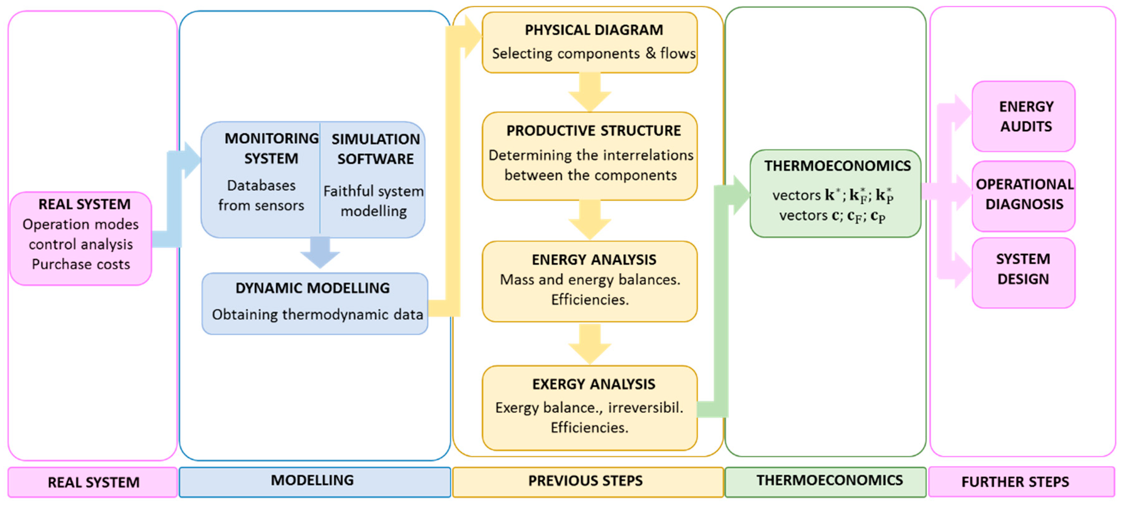
Once the productive structure is defined, thermoeconomics can be applied. In consequence, according to the irreversibilities encountered across the energy transformation chain (from generation to consumption), an exergy cost is allocated to each flow of the system that reflects the amount of exergy required to produce it. The unit exergy cost of each flow represents the amount of exergy required to obtain a unit of exergy of the flow (for all flows is expressed by vector k*) which increases while irreversibilities turn up. These unit exergy costs can be distinguished additionally in exergy costs of fuels (vector kF*) and products (vector kP*). Similarly, by a simple unit conversion from exergy units to economics ones, the unit exergoeconomic costs (expressed by vector c) can be calculated. Here again, the unit costs associated with the fuel and product of each component can be pulled apart (vectors cF and cP respectively).
Often the aim is to determine the cost of the final products of the system, which in the case of an energy supply system, are the cost of DHW, heating, cooling, ventilation and electricity. To calculate these costs, one must know the prices of the consumed resources (natural gas, diesel, electricity, biomass, etc.), and the investment costs of every equipment and further economic data (lifetime, interest rates, etc.). As already mentioned, thermoeconomic results can be used for energy audits, operational diagnosis or even system design purposes.
Figure 2 summarizes the whole methodology of thermoeconomic application. The figure distinguishes the main processes which are: (1) real system identification, (2) modelling of the facility and its components, (3) defining the physical and productive structure, (4) costs calculation and (5) implementing it for further application.
5. Case Study
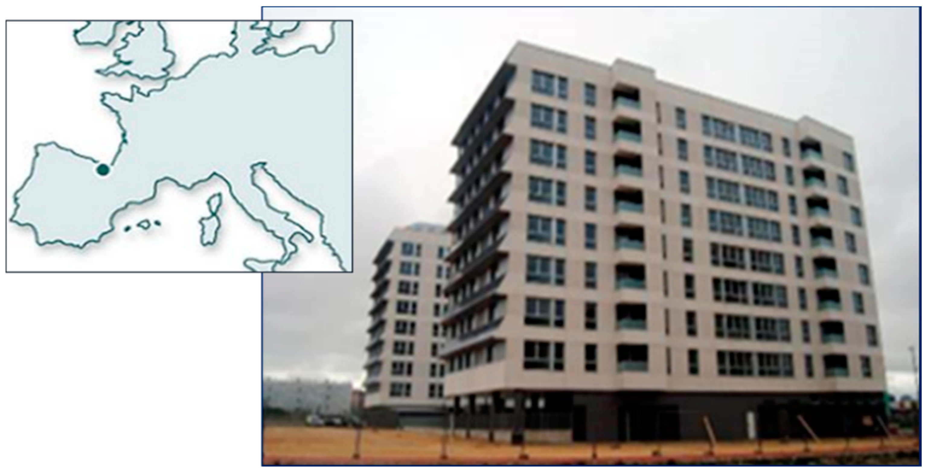
In the case analyzed in this work thermoeconomics is applied to three nZEB buildings located in Vitoria-Gasteiz (Basque Country), see
Figure 3, Ref [
31]. The acronym nZEB refers to a nearly zero energy building which aim is to provide the indoor comfort conditions with the lesser energy consumption as possible. If readers want a deeper definition of nZEB as well as the progress of their implementation in Europe, they can consult reference [
32]. Referring to the buildings, there are 171 dwellings, 3 shops and a private urbanization; there are also 176 garages with storage rooms together with the boiler room.
The façades are made up of prefabricated concrete panels with an interior formed by a plasterboard panel and high levels of insulation; its transmittance value is 0.35 W/m
2 K. Special attention has been paid to correctly insulating the edges of the slabs in the encounter with the concrete panels in order to minimize thermal bridges. Because of the same reason, the encounters of the exterior carpentry of the façade are also made very carefully. The exterior carpentry is made of aluminum with frames whose transmittance is 1.9 W/m
2 K. The frame and glass assembly has a transmittance for the gap of 1.5 W/m
2 K. In the case of the roof, the transmittance is less than 0.24 W/m
2 K; all these values were below the regulatory requirements at the time of construction, [
33].
5.1. Operation Mode and Control Analysis
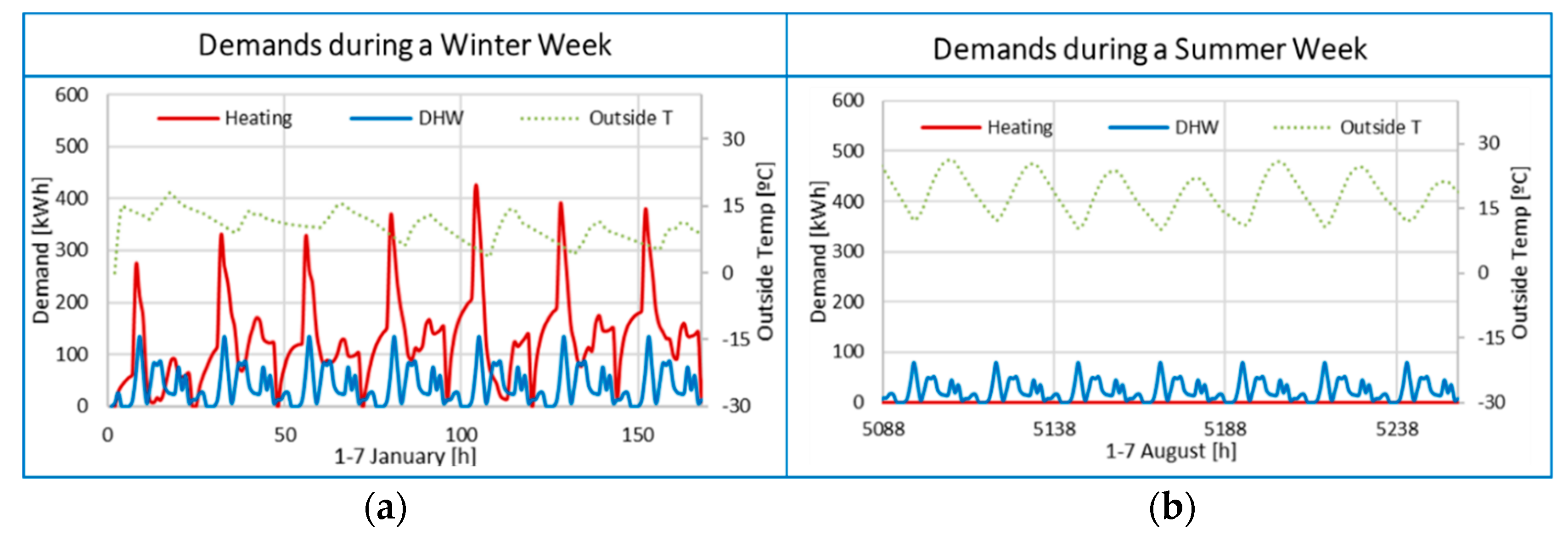
The thermal system is designed to supply the heating and DHW demands since, according to the climate data and placement of the buildings, no cooling is required for summer conditions. In Vitoria-Gasteiz, to summarize, summers are not very hot, winters are cold and it is partly cloudy all year. During the year, the temperature generally varies from 1 °C to 26 °C and rarely drops below −4 °C or rises above 34 °C; being the average temperature of 12 °C.
The generator units of the HVAC system are two high-performance natural gas boilers and two micro-cogeneration engines working between 80/60 °C temperature range. The boilers are programmed to work in cascade, and modulate their power from 320 to 500 kW; their energy efficiency varies from 92% (at full load) to 95% (at 30% load). Each of the combined heat and power engine can provide 5.5 kW of electricity, with a nominal electrical efficiency of 27%, and 12.5 kW of heat, with a nominal thermal efficiency of 61%.
The activation and deactivation of the micro-cogeneration engine circuit is muffled by a 3000-L tank connected to a heat exchanger [
34]. The water heated by boilers and the cogeneration units is afterwards separated in heating and DHW circuits. The first circuit is connected to the corresponding heaters of each dwelling while the DHW one is connected to a 3000-L storage tank. In addition, the building also has a series of photovoltaic panels on the south facade with 33.5 kW peak power [
35] (This work focuses only on the heating and DHW thermal demands so, as electric demand is not considered, the implications of photovoltaic (PV) panels are not taken into account. Nevertheless, the cogeneration engines produce simultaneously electricity, which is used as fuel of hydraulic pumps of the facility. Therefore, such electricity would be considered during the analysis).
The control system is programmed in such way that the priority is given to cogeneration engines, which are able to cover 90 % of the DHW demand. They turn on at any time when there is heating or DHW demand, since they are the priority units as they simultaneously produce electricity and heating. When the demand is not satisfied and more heat is required, the boilers are turned on.
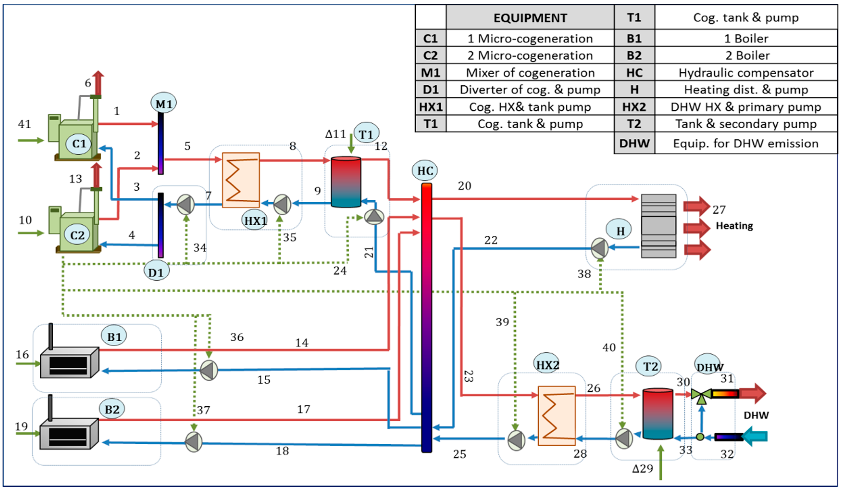
The simplified hydraulic scheme of the installation appears in
Figure 4, in which all the equipment and flows are labelled. The legend, in the upper and right part, includes the selected components and their assigned abbreviations.
5.2. Purchase Costs
The price of purchasing electricity is 22.33 c€/kWh, that of natural gas is 5.43 c€/kWh and mains water is 0.52 €/m
3; the service life of the installation is 20 years and the effective interest rate is 0.05. Based on the data obtained from the engineering company that developed the project,
Table 1 shows the investment cost of the components.
5.3. Dynamic Modelling
Considering the building architecture, Autocad software was used to build the geometric model of the buildings. Then, the physical properties of the envelope and the users’ profile were introduced through the TrnBuild interface of the transient simulation tool TRNSYS v17 [
36]. The weather data of Vitoria-Gasteiz was also included in the simulation by the Typical Meteorological Year provided by the software. Accordingly, the heating demand was calculated hourly. That consumption was compared to the monthly bills, which were at the same time related with specific meteorological conditions, in order to adjust the building-model parameters. In addition, the DHW demand was obtained following the recommendations given by the Spanish Institute for Diversification and Energy Saving (IDAE) [
37,
38] which considers the use of the building, the distribution of the dwelling and the number of tenants.
The heating and DHW demands and the outside temperature during a winter week (from 1 January to 7 January) and a summer week (from 1 August to 7 August) appear in
Figure 5. As mentioned, the electric demand is not included since only the thermal demand, covered by boilers and cogeneration engines, was analyzed.
Afterwards, a Simulation Studio interface was used to model the heating and DHW thermal facility. This tool enables the dynamic representation of the HVAC system by linking different types from the library or from user-made models. Each type corresponds to a specific component of the system and is based on a grey-box modeling. For space reasons, the method to validate the model does not appear along this work, but is the one developed in reference [
13], and appears also in reference [
5]; if the reader wants to deepen on model validation with Trnsys reference [
39], can also be read.
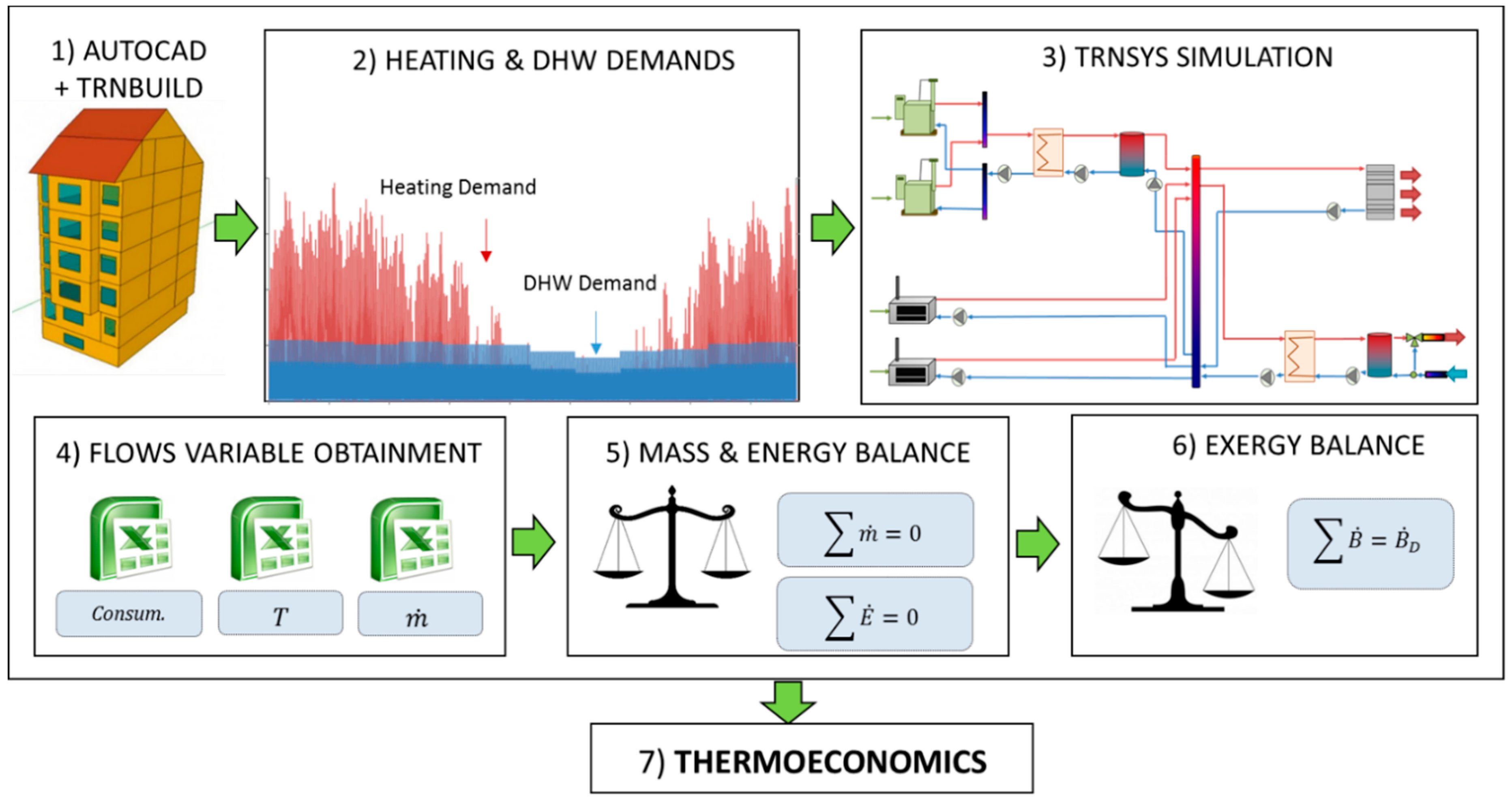
Figure 6 depicts the schematic diagram to be followed.
Throughout the 8760 h of the yearly simulation (starting from 1 January until 31 December), the required data for the mass, energy and exergy balances were obtained from the software, being basically the flow rates and temperatures of each flow. As already mentioned in
Figure 2, this is the previous step required for applying thermoeconomic in building thermal systems.
6. Numerical Results
This section includes the numerical results of thermoeconomic application.
6.1. Energy and Exergy Analysis
According to
Figure 2 the first step deals with the definition of the physical structure of the installation. This is simply done by detecting the incoming and outgoing flows of each component. Then, the second step requires the definition of the productive structure, which is based on the functional analysis and can be different according to the research purpose.
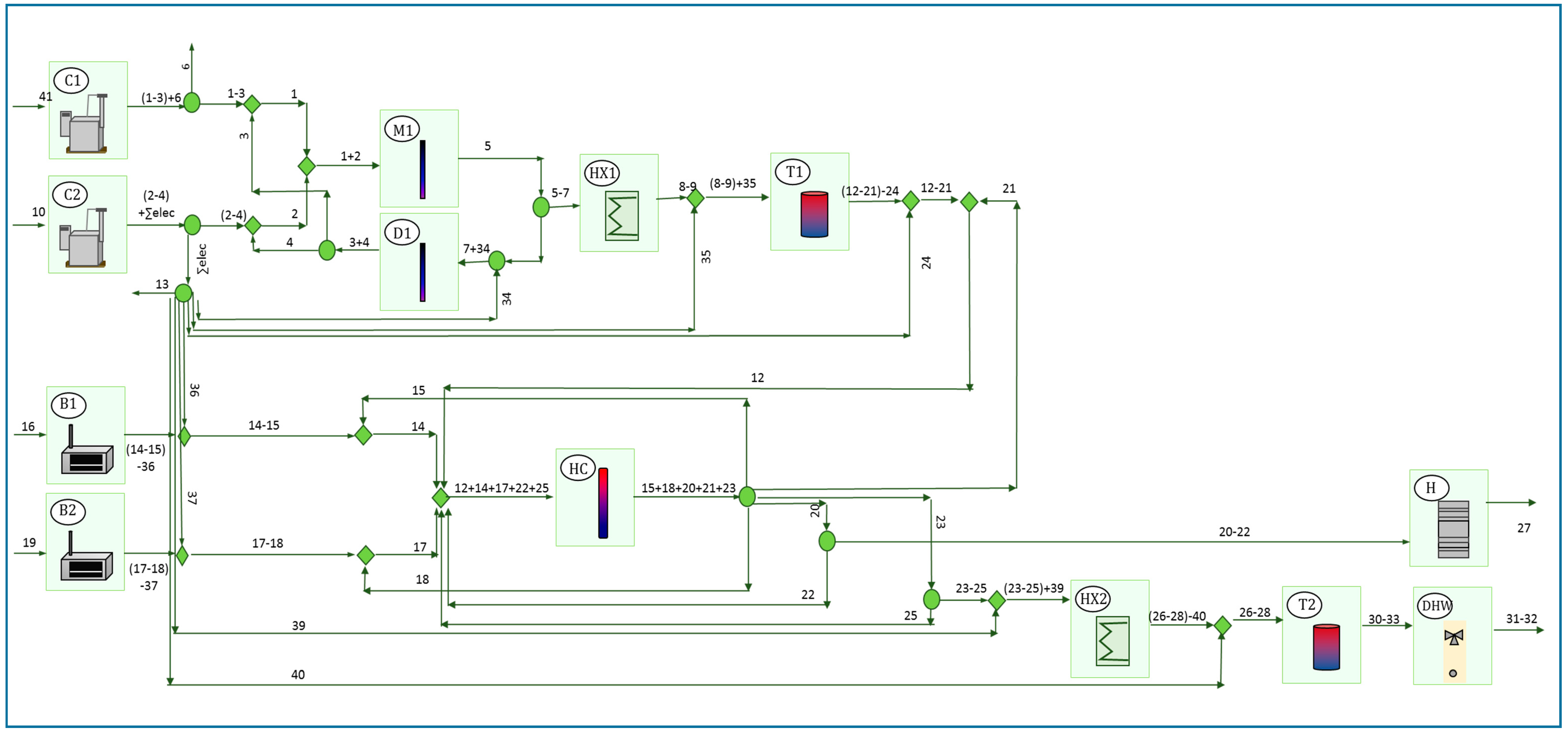
Figure 7 represents the structural diagram chosen for the case study: each main component is represented in a square composed by an entering flag (which represents the fuel, F) and an outgoing flag (the product, P); besides, diamonds and circumferences are used to reflect junctions and bifurcations of the flows. As mentioned previously, the ratio P/F reflects the efficiency of each component. According to this productive definition,
Table 2 contains the annual cumulative energy values of the fuel and the product of each main component. The numerical values of this table supports the introduction of different options for defining F and P.
As can be seen, the fuel of M1 is high in comparison with the energy product of the cogeneration engines, which is precisely related to the definition of each F and P. The product of cogeneration engines are defined as the enthalpy increment in between the outgoing and the incoming water flow plus the produced electricity. That is, PC1 = (E1 − E3) + E6 and PC2 = (E2 − E4) + [E6 + (E24 + E34 + E35 + E36 + E37 + E38 + E39)]. However, the fuel of M1 is: FM1 = E1 + E2 and that is why both values cannot be directly compared.
Something similar happens in HC. The fuel was defined as the sum of incoming flows, FHC = E12 + E14 + E17 + E22 + E25, and the product as PHC = E15 + E18 + E20 + E21 + E23. However, another option can be to define FHC such as FHC = (E12 − E21) + (E14 − E15) + (E17 − E18) and PHC = (E20 − E22) + (E23 − E25) and different thermoeconomic results would appear.
Obviously, the final products of the system are heating (E27), DHW (E31−E32) and the electricity generated in the micro-cogeneration engines (E6 + E13). Since pumps are powered by this electricity, the net electrical production is equal to the electricity generated by both engines minus the pumps’ consumption, (E24 + E34 + E35 + E36 + E37 + E38 + E39). Then, the total resources consumed by the installation include the fuel of the boilers plus the fuel of the cogeneration engines (E41 + E10 + E16 + E19), since the pumps are powered by the electricity generated in the cogeneration units.
According to the efficiency values of
Table 2 one can see that the diverter D1, mixer M1, hydraulic compensator HC and heat exchangers HX1–HX2, are very energy-efficient, and even some of these components have an efficiency of 100%, as they are practically adiabatic. Similarly, the efficiency of the tanks T1–T2 are close to unity, and the energy efficiency of the internal combustion engines C1–C2 is also high, around 80%.
The pumps were not considered as components but as part of other components and then the electricity consumed by the circulation pumps is included in that of those components. This is done to avoid the calculation of the mechanical energy along the system, since the pressure changes are negligible in almost all the rest of the equipment. After all, for a circulation pump the fuel F is the electrical energy consumed and the product Ps is the mechanical energy increase of the flow between the inlet and outlet. Therefore, by this approach the mechanical energy did not have to be considered separately in this case study.
In the same way as with energy, the exergy of every flow was calculated and the yearly-cumulated values were obtained. Therefore, the fuel and product of each component were calculated as well as the P/F exergy efficiency ratio; the results appear in
Table 3.
Compliant with the results, we have seen that the energy efficiency of boilers are higher than those of cogeneration engines, while the opposite happens with the exergy efficiencies. This means that, even if in terms of energy boilers seeming to have better performance, the real losses are higher there than in cogeneration engines. After all, cogeneration engines simultaneously produce thermal energy and electricity and the last one is a high-quality energy.
The energy efficiency for electricity production in the cogeneration units is 39.8% and the energy efficiency 38.3%, the efficiency for producing heat and DHW is 86.4%, and the exergy efficiency is 4.2%. Finally, as a whole, the average energy efficiency of the energy supply system is 89.4% whereas its exergy efficiency is 7.1%.
6.2. Thermoeconomic Analysis
Once the balances of the first and second laws were calculated, the next step deals with the application of thermoeconomics. Consequently, by means of the productive structure, the vector of unit exergy costs of fuel and product (k
F* and k
p*) were calculated.
Table 4 shows the obtained average annual values for each component.
These vectors allow mapping the cost formation process following two main facts:
On one side, for each i-th component, the difference between the unit exergy cost of the product (kPi*) and the unit exergy cost of the fuel (kFi*) sets forth the cost of irreversibilities in the i-th component itself per unit of product, since .
On the other side, the difference between the unit exergy cost of the outgoing product of the i-th component (kPi*) and the exergy cost of incoming fuel of the j-th component (kPj*) refers to the irreversibilities associated with the productive chain structure. That means that while the productive process is going downstream the irreversibilities accumulate so the cost increases. The fuel in the boilers and cogeneration engines (natural gas) are considered as inputs to the system so, in the absence of external assessment, its exergy cost is equal to 1. By contrast, the hydraulic pumps are fed by the electricity coming from the micro-cogeneration engines so their exergy cost is equal to the cost of the electricity cogenerated kFpump* = kPcog*.
When considering
Table 4, it is worth emphasizing that the unit cost of the product of the emitting device, the final component in the energy chain, has increased significantly in respect to the unit cost of fuel, going from
kFH* = 6.71 to
kPH* = 28.65. This large increment is because the indoor air is included in that final component, so its product is very low as it is equal to the exergy of heating and the operating temperature is close to the environmental temperature. It is worth noting that the unit exergy cost of the fuel in DHW production is higher than the one of heating
kFDHW* > kFH*. This is because DHW generation requires more components than heating and, therefore, it accumulates more irreversibilities and cost increases. Consequently, the mean value of the exergy unit cost of heating is equal to 28.65, the unit DHW cost is 14.9 and the electricity cogenerated has an average unit cost of 2.8.
Finally, the next step deals with translating the exergy unit costs to economic unit costs by means of the economic data.
Table 5 shows the average annual unit costs required for producing heating, DHW and cogenerated electricity (referred per unit of energy). The annual cost for the whole building and the cost for each dwelling are also shown. These costs are calculated considering the acquisition costs of
Table 1 and the unit price of electricity and natural gas; nevertheless, a deeper analysis can be undertaken if life-cycle analysis (LCA) is carried out. Indeed, the cost of environmental impact is calculated in the same way but instead of considering the economic values, the whole life impact is taken into account (through an eco-indicator), from the cradle to the grave.
Finally,
Table 6 shows the savings obtained with cogenerated electricity (which corresponds to the by-product obtained simultaneously when heating demand is being covered). This value is obtained by subtracting the cost of cogenerated electricity from the cost of direct purchase from the grid. Although the cogeneration engines present a relatively reduced working time (1477 h per year for both engines), they still save an important amount of money. After all, the electricity purchased from the grid with a price of 22.33 c€/kWh is replaced by the cogenerated electricity at a unit cost of 11.37 c€/kWh.
According to the results, the micro-cogeneration engines are more efficient than boilers, since they have higher exergy efficiency, as they produce simultaneously heat and electricity. Therefore, if only exergetic cost is considered, producing heat with cogeneration would always be more beneficial because there are less irreversibilities. However, cogeneration requires a relatively high investment, if we compare its purchase cost with the cost of buying a boiler with the same heating power. Nevertheless, the annual savings obtained with electricity cogenerated are 3226 €, as shown in
Table 6.
On the other hand, one cannot forget that the electricity demand can also be fulfilled by the production of the PV panels, and that option should also be considered. After all, the best configuration and the best control that minimizes the energy consumption needs to be analyzed, but that is beyond the scope of this work.
7. Conclusions
Even if exergy analysis is a widely used methodology in industrial processes, it is rarely used in the building sector. Therefore, this work is focused on this sector and aims to achieve energy savings in buildings, as well as economic savings and a reduction of CO2 emissions, by using second law methodologies.
To this end, a real thermal installation, including boilers and cogeneration engines, covering the heating and DHW demands of several apartment buildings was analyzed. Then, with the help of thermoeconomics, the irreversibility associated with each component was calculated and for each flow and particularly for the final products, the unit exergy costs as well as the exergoeconomic costs were calculated.
Although the average energy efficiency of the cogeneration engines (80%) is slightly lower than that of the boilers (92%), the results obtained prove that micro-cogeneration engines not only save energy (weighted by its quality) because they have better exergy efficiency (36%) than boilers (15%), but economically are attractive, even if they require relatively higher investment. Indeed, according to the results, the combustion boilers are the lesser efficient components. Additionally, exergetic and exergoeconomic costs provide very interesting information because they show us the formation cost of each flow and particularly that of the final products of the system, that is, the cost of electricity, heating and DHW. Exergetic unit costs are higher in heating (28.65) than in DHW (14.90) due to the irreversibilities related to the temperature difference among the indoor air and the heating hot-flow; however, as exergoeconomic cost includes the acquisition cost of the equipment, the values are closer (7.42 c€/kWh for heating and 7.25 c€/kWh for DHW). Additionally, we prove that generating electricity through micro-cogeneration engines is cheaper (11.37 c€/kWh) than purchasing it from the network (22.33 c€/kWh).
Hence, with the application of thermoeconomics, it is possible to go deeper and to understand more accurately the cost-formation process, either in energy or in economic units. Consequently, the impact of irreversibility in each component on the total heating and DHW cost may be known.
As a conclusion, we can say that this methodology underscores the necessity to adapt the energy quality between generation and demand, encouraging the use of low-temperature heating terminals.
8. Further Research Lines
Aiming at the practical application of this methodology in the building sector, thermoeconomic software is being developed for cost accounting and diagnosis in buildings’ facilities. Such a software, with the data obtained from a monitoring system, can locate the abnormal behavior of a component and avoid unnecessary interruptions or cost losses, so it can become a solid management tool for building maintenance and optimization.
Another prospect involves the improvement of thermoeconomic diagnosis in any facility. For example, the air-conditioning system of an office is a complex one, and its thermoeconomic behavior has been rarely analyzed; therefore, it should be studied in depth.
In addition, quantifying environmental impact through exergoenvironmental analysis can also be used in a further supplementary study to obtain the global energy, economic and environmental profile of the system. In this case, the analysis will be carried out through the entire life of the system, starting from its conception and ending with its decommissioning.


