Experimental Investigation of Magnetic Particle Movement in Two-Phase Vertical Flow under an External Magnetic Field Using 2D LIF-PIV

Abstract

In this study, we experimentally investigated magnetic particle movement in two-phase flow under an external magnetic field. According to Faraday’s law, the alignment of a magnet is important for power generation. For high generation, it is important to understand how magnetic particles move in two-phase flow. The rotationality could be determined by observing a single particle; however, this is impossible due to the flow conditions. In this study, we estimated nonrotationality based on the vorticity. To eliminate scattered light and improve the signal-to-noise ratio, the laser-induced fluorescence particle image velocimetry technique was used. The solenoid nozzle has a hydraulic diameter of 3 mm. Its surface is covered with a coil with a diameter of 0.3 mm. The average diameter of a magnetic particle is 1.2 μm. The excitation and emission wavelengths are 532 and 612 nm, respectively. A thin laser sheet setup was configured. The laser sheet was illuminated on both sides to prevent shadows. The images were captured at 200 μm away from the wall and center of the nozzle. To estimate the decrease in vorticity, the theoretical and single-phase non-magnetic and magnetic particles are compared. The vorticity of magnetic particles is reduced by the external magnetic field.

1. Introduction

Ferrofluid is used in a variety of fields, such as drug delivery, heat transfer, energy harvesting, microdevices, and separation, due to physical limitations and the control of existing fluid [1,2,3,4,5,6,7,8,9]. Recently, magnetic nanofluids with magnetic nanoparticles dispersed in oil or water have been used in areas to increase the efficiency of power generation systems or gain new energy. In addition to the generation of power through the back-and-forth movement of magnetic flow, the generation of power through changing the magnetic field using air bubbles can also be used. Yun et al. [10] created a ferrodynamic system that generates power by moving a stationary ferrofluid inside a magnetic field and using air droplets to cause a change in the magnetic field. This system requires the continuous injection of air bubbles using an external source for power generation. To simplify and improve the efficiency of the conventional heat waste recovery system based on this principle, Kim et al. [11] designed an inductive system. This system applies Faraday’s law instead of using a turbine for power generation, applying convection via a temperature difference for the working fluid forced to circulate by a pump. In this inductive system, a magnet that moves inside the coil is replaced with ferrofluid. The magnet is placed outside the coil to magnetize the ferrofluid. This approach shows that the ferrofluid circulating in the closed loop generates power by inducing a magnetic field change from the bubbly flow generated when the fluid is boiled by an external heat source. Furthermore, Kim et al. [11] demonstrated that it is impossible to generate power using only the flow of ferrofluid and that a two-phase flow with a mixture of air is required instead.

Many studies on ferrofluid in single-phase flow have been carried out in recent years. There has been little research on two-phase flow. To enhance the heat transfer effect, ferrofluid affected by an external magnetic field in two-phase flow was numerically researched [12,13]. Unlike those on single-phase flow, numerical studies on two-phase flow are heavily simplified, and the actual flow is much different. For flow control in microfluidic chips, ferrofluid slug flow, which is influenced by the external magnetic field inside the T-junction, was experimentally studied [14]. There is still a great need for research on ferrofluid affected by external magnetism in two-phase fluid flow. In energy harvesting research, most studies have only researched the possibility of power generation methods or the amount of power able to be generated in ideal situations. The flow of internal ferrofluid has not been researched thoroughly.

A ferrofluid with an external magnetic field that flows inside a solenoid nozzle can be measured by particle image velocimetry (PIV), which is a noncontact measurement method. Since the inside of the solenoid nozzle becomes a two-phase flow that mixes with air, light is scattered by the air, which increases the amount of errors or makes it impossible to accurately observe the particles. A technique that can eliminate this phenomenon is laser-induced fluorescence (LIF). LIF is a spectroscopic technique that detects radiation emitted from an object after exciting a molecular target with a laser [15]. In this technique, a tracer particle is dyed with a fluorescent dye and excited with the laser. The emitted fluorescent signal is then measured. LIF can pass through or reflect a specific wavelength with an optical filter. Hence, it can remove scattering from the gas or from the liquid surfaces and measure a fluorescent signal with a uniform background [16,17]. Murgan et al. [18] measured bubble column flow using LIF-PIV. An appropriate image processing method was developed. Siddiqui et al. [19] separated air and water with two cameras using the LIF-PIV technique in horizontal two-phase flow. Petrosky et al. [20] showed that fluorescent signals from fluorescent particles were weaker than 320 ± 10 times Mie scattering on average, but fluorescent PIV could measure surfaces closer than Mie scattering. Fluorescent PIV in this configuration led to velocity vector validation rates of more than 20 times those of Mie scattering in the boundary layer region.

Some studies have used external magnetic fields to efficiently control fluid. N₂ gas was injected through vertically placed tubes to measure the flow of nonconductive air under the influence of a magnetic field, and N₂ flow was visualized using PIV techniques. Through magneto-aerodynamics research, Xiaodong et al. [21] showed that PIV techniques are effective tools. Takeuchi et al. [22] measured internal flow using PIV to understand turbulent flow under external magnetic fields. Due to limited internal space, special optical devices have been designed for laser investigation. A magnet is placed outside the horizontal tube and enclosed with a square tube to prevent distortion. Measurement of the internal turbulent flow showed that turbulence was reduced by external magnets. Kim et al. [23] measured the flow around a single particle and compared it with simulation results using a rotating 200 nm magnetic microparticle under low-Reynolds-number flow via μPIV with typical fluorescence. It was also found that the flow produced by two identical particles rotating in one unit was similar to that of a single particle with a twice diameter. Gilard et al. [24] showed that the inflation of the magnetic field on the liftoff and blowout properties of a methane/air co-flow diffusion flame is effective. The research used PIV techniques to measure a flame surrounded by magnets on the outside. The results showed that the magnetic gradient minimizes the lift-off head and increases the flow rate emitted. Munhoz et al. [25] measured the asymmetric gas flow affected by the magnetic file placed around the cylinder and the aerodynamic force acting on the cylinder using the PIV technique.

Tan et al. [26] measured the movement of microswimmers affected by an external magnetic field using μPIV techniques. Previous studies showed that external magnetism placed outside of a flow field can effectively control a flow field. The PIV technique allows the measurement of flow fields under this external magnetic field.

Table 1. A summary of previous studies on the effects of external magnetic field.

Author	Technique	Phase	Seed Particle	Magnetic Flux Density	Year	Method
Xiaodong et al. [21]	2D PIV	Single	CO2	1.5 T	2004	Experiment
Takeuchi et al. [22]	2D PIV	Single	Methyl methacrylate–ethylene glycol dimethacylate copolymer	2 T	2007	Experiment
Yang et al. [27]	2D PTV	Single	FeCl3, FeCl2–4H2O	Up to 470 mT	2007	Experiment
Gilard et al. [24]	2D PIV	Single	Methane/air	0.35 T	2008	Experiment
Takeuchi et al. [28]	2D PIV	Single	Li2BeF4	2 T	2008	Experiment
Aminfar et al. [29]	Two-phase mixture	Liquid–solid	Sea water, Fe3O4	6E5 A/m	2012	Numerical
König et al. [30]	LDV-PS *, 2D-PIV	Single	NaOH	Electrode (500 mA)	2013	Experiment
Zeng et al. [6]	Bright-field microscope	Single	EMG 408, Tween 20	1.32 T	2013	Experiment
Asfer et al. [1]	2D $\mathsf{\mu }$PIV **	Single	Fe3O4	0.15 T	2015	Experiment
Ali et al. [23]	2D $\mathsf{\mu }$PIV	Single	Fluorescent 200 nm	15 mT	2016	Experiment, Numerical
Munkhoz et al. [25]	2D PIV	Single	Arc gas	0.1 T	2017	Experiment
El-Amin et al. [13]	CFD ***	Single	Ferromagnetic fluid	0.2 T	2018	Numerical
Hangi et al. [31]	Two-phase mixture	Liquid–solid	Fe2Mn0.5Zn0.5O4 magnetic nanoparticles	1.2E6 A/m	2018	Numerical
Shahsavar et al. [32]	Two-phase mixture	Liquid–solid	Mn–Zn ferrite ferrofluid	Up to 0.1 Am	2018	Numerical
Weerasiri et al. [33]	2D PIV	Liquid–gas	Hollow glass spheres 10 μm	Up to 0.72 T	2018	Experiment
Munkhoz et al. [25]	2D PIV	Single	Arc gas	0.1 T	2019	Experiment
Tan et al. [26]	2D $\mathsf{\mu }$PIV	Single	Fluorescent 200 nm	Electromagnetic	2019	Experiment

* Laser Doppler Velocity Profile Sensor ** Micro Particle Image Velocimetry *** Computational Fluid Dynamics.

is a summary of previous studies on the effects of external magnetic field. Numerous numerical and experimental studies on ferrofluid in single-phase flow have been performed in previous studies. Very few of them have adopted liquid–gas two-phase flow measurement. In this study, a closed-loop power generation system that uses waste heat, as proposed by Kim et al. [11], was configured. In this system, single- and two-phase flow occur. Kim et al. [11] used experimental and numerical simulation techniques to show that generation is only possible in two-phase flow. If the characteristics of magnetic particles for two-phase flow are known, an efficient nozzle design is possible. The details of this system are described in the next section. Magnetic particle flow without an external magnetic field has the same rotational properties as nonmagnetic particle flow. If it is affected by the external magnetic field, it will be aligned due to the magnetic force, and the degree of rotation is expected to be much lower. The rotationality of the magnetic particle could be determined by observing a single particle alone, but it is realistically impossible to measure a single particle due to its high velocity, small diameter, and complex flow. This study estimates nonrotationality based on vorticity. To verify the effect of the external magnetic force, the two-phase flow is compared to a fully developed theoretical model, nonmagnetic, and magnetic particles in single-phase flow.

2. Experimental Apparatus and Procedure

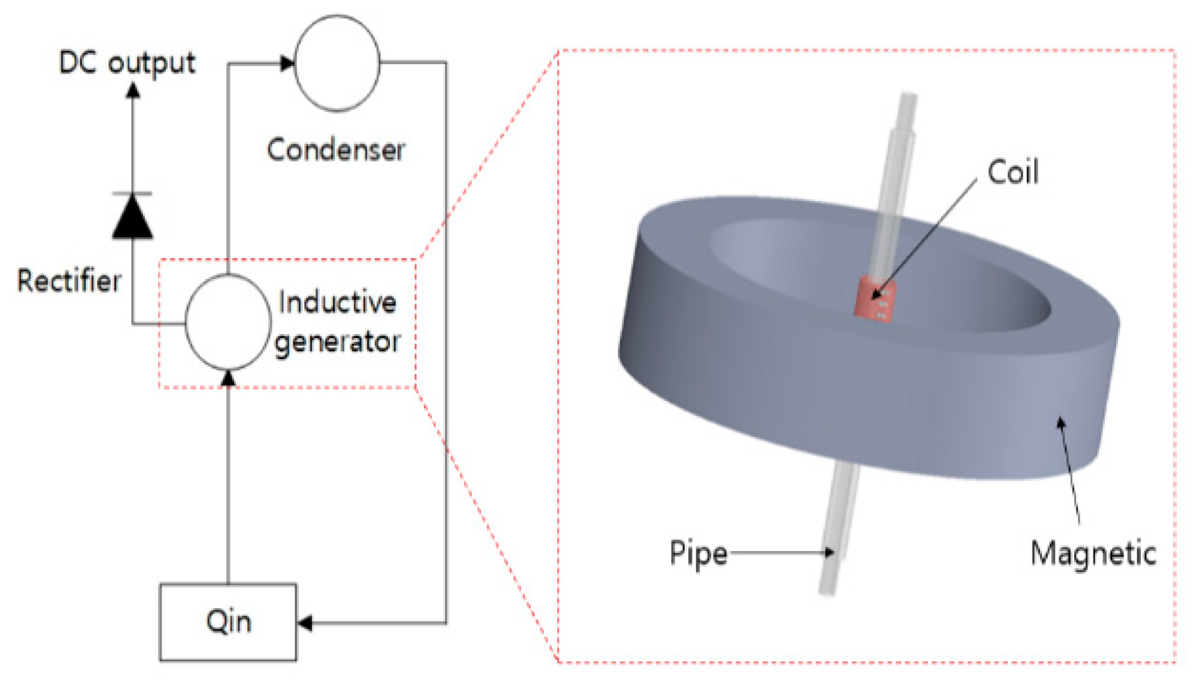
2.1. The Organic Inductive Cycle (OIC)

Figure 1 shows a schematic of the Organic Inductive Cycle (OIC) power generation system proposed by Kim et al. [11]. The energy is input through the bottom of the cycle using external waste heat. The ferrofluid circulates inside the closed loop because of convection due to the temperature difference. A condenser is placed at the top, and the flow changes from two-phase flow to single-phase flow. The two-phase flow phenomenon presents differently depending on the height from the energy input area. The generator is placed between the energy input area and the condenser where the two-phase flow appears. The principle of power generation is explained by Faraday’s law of electromagnetic induction. The induced current is proportional to the magnitude of the magnetic field change, as represented in Equations (1) and (2) (Faraday’s law):

$${\displaystyle \underset{c}{\int }E\cdot dl}=-\frac{d}{dt}{\displaystyle \underset{s}{\int }B\cdot ds}=-N\frac{d\mathrm{\Phi }}{dt},$$

(1)

$$\mathrm{\Phi }=BA\cos \theta .$$

(2)

In these equations, E is the electric field, B is the magnetic field, N is the number of turns of the coil, Φ is the magnetic flux, t is the time, A is the area, and θ is the angle between the magnetic flux and the magnet. According to this equation, a large number of coils and the higher the amount of change in the magnetic flux, the smaller the time change and the more power that is generated. However, due to the limitation of the system, that is, the speed of the magnetic fluid passing through the power generation unit, the internal maximum velocity is within 1 m/s. According to Kim et al. [11], the magnetic field saturation of a magnetic particle is approximately 0.23 T. As the number of particles passing through the coil increases, more power generation occurs, but research on the optimal particle concentration is still needed because high particle density makes the flow rate low.

Based on the principle introduced by Faraday’s law, a magnet should be placed outside of the power generation area, and a solenoid nozzle wound with coil should be placed inside the magnet. When the ferrofluid passes through the coil, it is magnetized by the external magnet and generates power. Inside the power generation area, there is a rotating flow field that is not affected by the external magnet and a nonrotating flow field in which the rotation property is significantly decreased by the effect of the external magnet. To increase the amount of power generated, the ferrofluid must be as vertically aligned with the coil as possible when it passes through it. In other words, if the ferrofluid has a high nonrotation property, the amount of power generated will also be high.

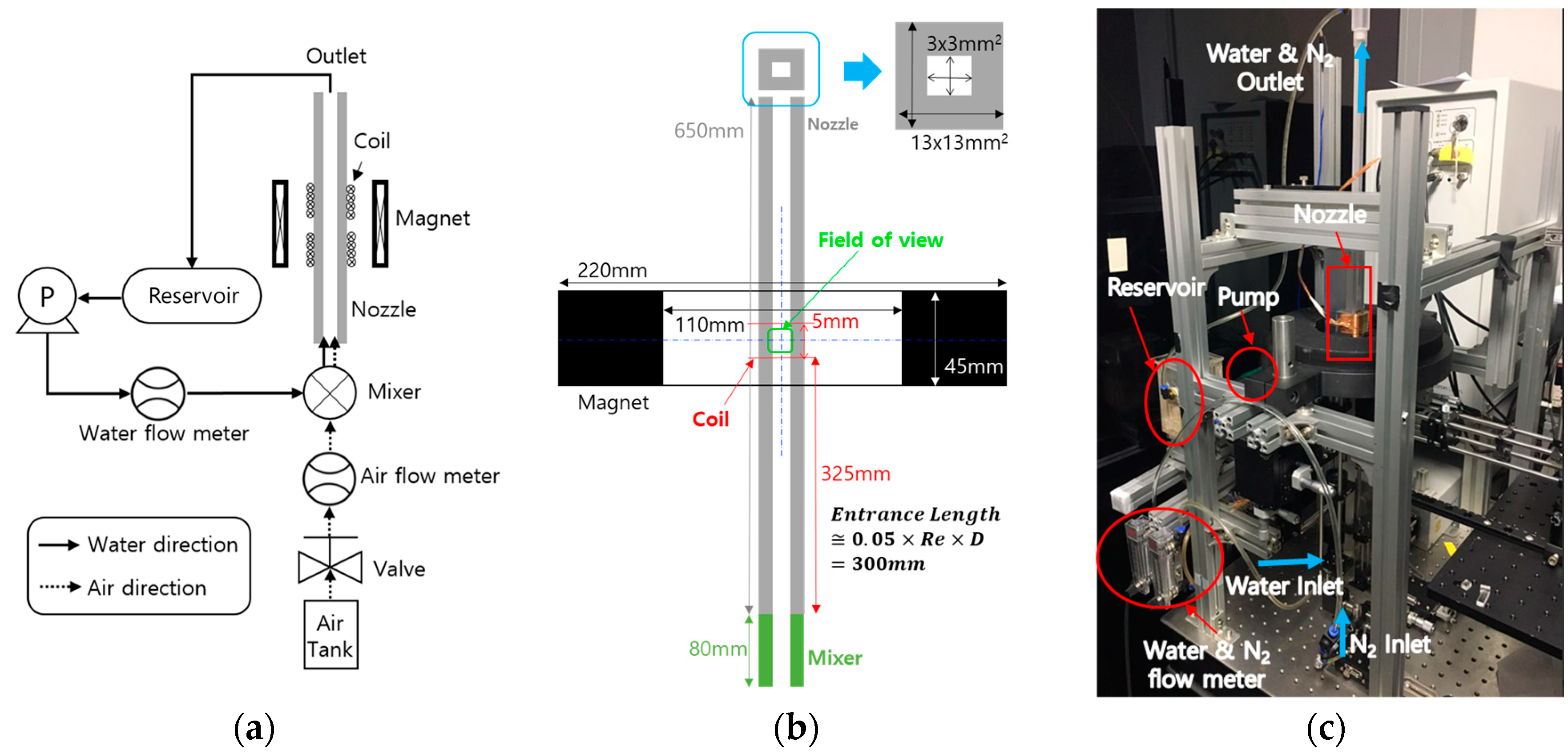
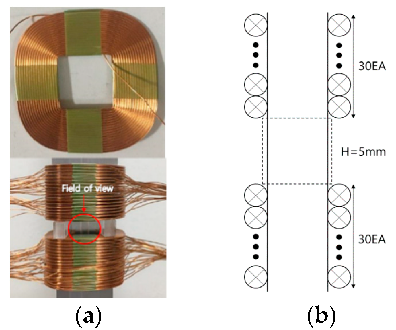
2.2. The Two-Phase Flow Circulation System

In this study, which was performed for two-phase liquid–gas vertical flow, an OIC system was implemented. Figure 2a is a schematic of the two-phase flow circulation system, in which the internal magnetic particles were circulated by a pump (PM-015NM, Wilo) and a ratometer. To implement the two-phase flow, nitrogen (N₂) was injected into the nozzle from the compression tank. The mixture of water and N₂ passed through the nozzle and returned to the reservoir. Magnetic particles were recirculated. The visualization window for measuring the flow of internal magnetic particles had no coil wound around an area that stretched 5 mm in height (Figure 2b). The inside dimension of the rectangle solenoid nozzle was 3 × 3 × 250 mm³. The wall thickness was 5 mm. For the inlet area, a 200 mm long pipe with a hydraulic diameter of 3 mm was connected to either side. The coil consists of 60 spans in total with 30 spans at the top and 30 spans at the bottom. Each span comprised 35 turns and had an outer diameter of 0.3 mm (Figure 3). A coil was wound around the outside of the solenoid nozzle, as shown in the cross section presented in Figure 3b. The magnets used for magnetic field formation were installed outside of the nozzle. The magnets were made of neodymium (OD 220 × ID 110 × T 45 mm³). The central magnetic force, measured using an FW Bell 8030 Tesla Meter, was 0.23 T. Figure 4 shows the magnetic flux density profile determined by numerical simulation. The magnetic flux density was 2300 G at the center. For inlet conditions, the water velocity was 0.67 m/s, Re 2000; the bubbly flow N₂ velocity was 0.093 m/s, Re 18; and the slug flow N₂ velocity was 0.926 m/s, Re 30. The average diameter of magnetic particles was 1.2 μm (Spherotech, Fluorescent Nile Red Carboxyl Magnetic Particles, FCM-1052-2, USA, excitation 532 nm, emission 612 nm). After the particles were placed in deionized water, they were sonicated for 15 min to prevent particle aggregation. The circulated deionized water came to a total of 200 mL. The concentration of magnetic particles was 0.001% (w/v).

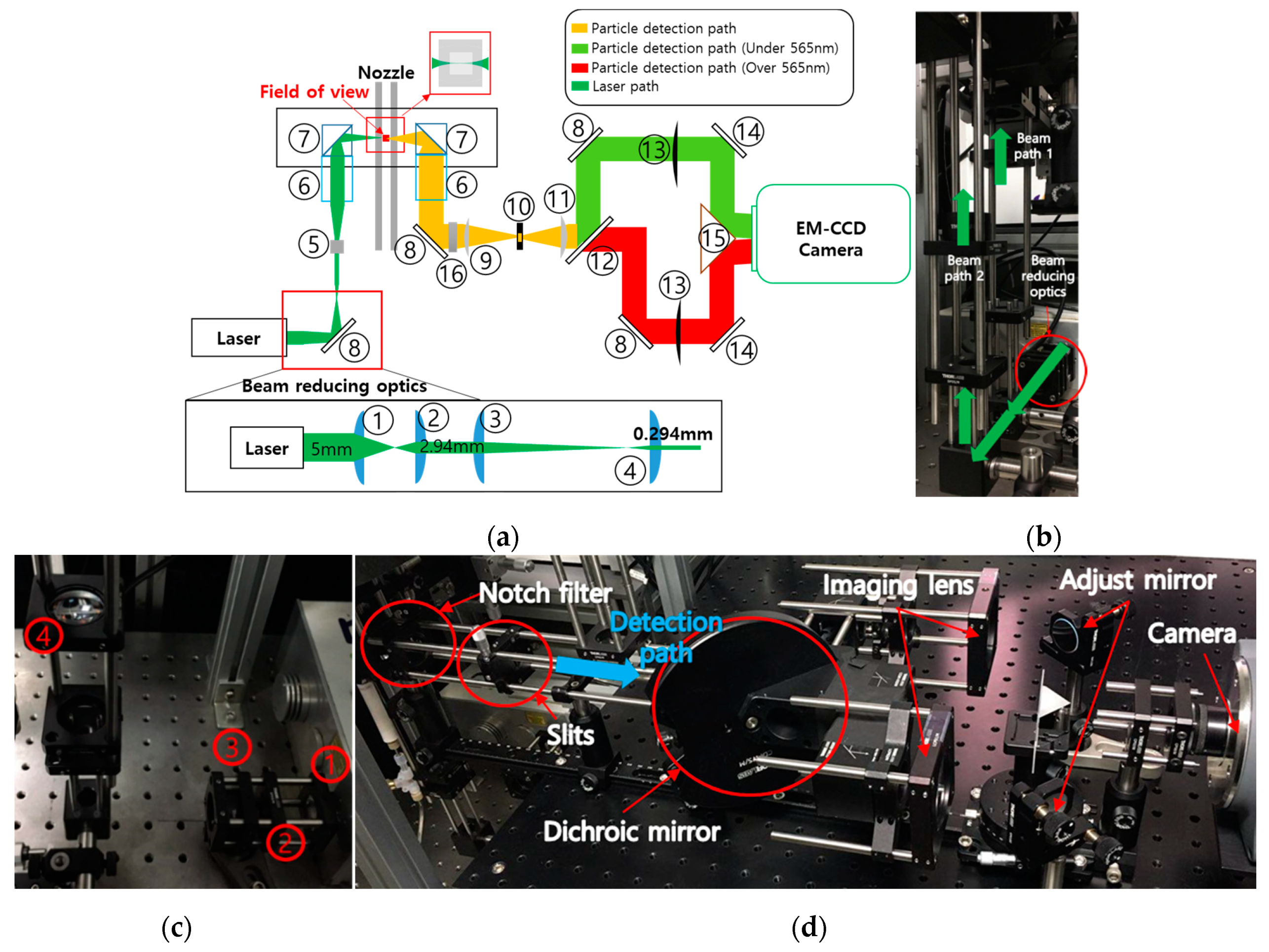
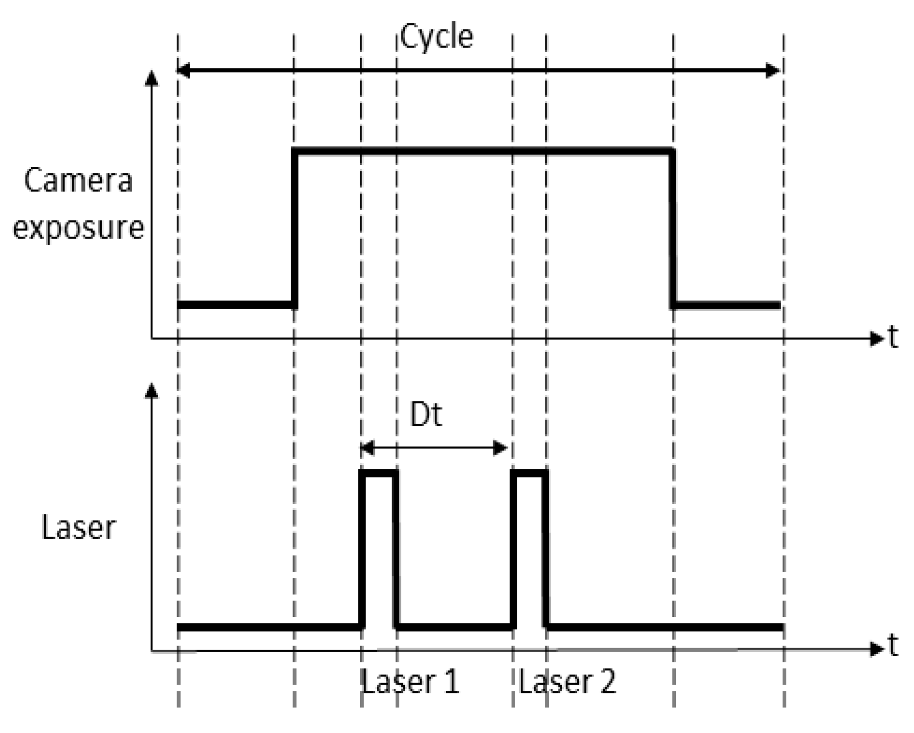
2.3. The LIF-PIV Setup

Figure 5 shows a schematic of the LIF-PIV setup. For future research, a two-color setup was configured. This setup allows for one- and two-color flow measurements with dichroic filter replacement. In this study, the one-color setup was used. In thick laser sheets, defocused particles can be observed and the particles overlap, which either disables or lowers the accuracy of the calculation. To observe particles with 1.2 μm diameters, the laser diameter was reduced from 5 mm to 0.254 mm through a combination of optical lenses. The reduced-diameter laser took on a sheet form with a 30 degree angle laser-line-generating lens and passed through an objective lens (Mitutoyo, 10 × F 20 mm, numerical aperture (N.A.) 0.28, working distance (WD) 34 mm). The laser was then bent at a right angle through a prism and mirror before illuminating the nozzle. In this experiment, the fluorescent signal area to be reflected was widened, and the laser illuminated both sides of the nozzle to prevent the creation of shadows from N₂ bubbles or particles.

For particle detection, the same objective lens used for the thin light sheet was used. The laser wavelength band reflected from N₂ bubble surfaces was eliminated by installing a notch filter in the back of the object lens. A camera with high quantum efficiency (QE) was used because the laser exposure time was very short (several tenths of nanoseconds) and the fluorescent signal area was small. An electron multiplying (EM)-CCD camera (Hamamatsu, C9100-23B ImagEm X2, Iwata city, Japan), 512 × 512 pixels², QE 99%, max 1076 frame/s) was used in this experiment. Figure 6 shows the timing used in the experiment. Since the EM-CCD camera does not have a double shutter mode, the first and second lasers were illuminated while the camera shutter was open. To synchronize the camera and the laser, a digital delay pulse generator (BNC Model 505, CA, USA) was used. The synchronization cycle was 10 Hz, and the time interval for the first and second lasers was 15 μs.

Table 2. A list of the optical parts used in the LIF-PIV setup.

No.	Manufacturer, Model	Specifications
1	Thorlabs, LA1252-A, Plano convex lens	F * 25.4 mm, D ** 25 mm
2	Thorlabs, LA1540-A, Plano convex lens	F 15 mm, D 12.5 mm
3	Thorlabs, LA1484-A, Plano convex lens	F 300 mm, D 25.4 mm
4	Thorlabs, LA1805-A, Plano convex lens	F 30 mm, D 25.4 mm
5	Edmund Optics, 43–473, Full fan angle laser line generator lens	30 degree
6	Mitutoyo, Plan Apo infinity corrected long working distance(WD) objective lens	10×, N.A. 0.28, WD 34 mm
7	Thorlabs, MRA25-E02, PS911, Right angle prism + right angle prism mirror	25 mm
8	Thorlabs, CCM1-E02/M, Cube-mounted turning prism mirror with 50:50 beam splitter and prism mirror	565 nm
9	Thorlabs, LA1509-A, Plano convex lens	F 100 mm, D 25.4 mm
10	Thorlabs, VA100C/M, Adjustable mechanical slits	30 mm
11	Thorlabs, LA1433-A, Plano convex lens	F 150 mm, D 25.4 mm
12	Thorlabs, CDFW5/M, Manual dichroic filter wheel	30 mm, 5 filters
13	Thorlabs, LA1461-A, Plano convex lens	F 250 mm, D 25.4 mm
14	Thorlabs, BB1-E02 Broadband dielectric mirror	D 25.4 mm
15	Thorlabs, MRAK25-P01, Knife-edge right prism	25 mm
16	Semrock, NFD01-532, Notch filter	532 nm

* Focal length ** Diameter.

shows a list of the optical parts used for the LIF-PIV setup in Figure 5a.

3. Results and Discussion

Figure 7 shows a raw image captured in the bubbly flow. The raw image shows two identical particles because the laser was emitted twice while the camera shutter was open, causing the particle to be captured twice. The bubble is located in the top and bottom parts of the image, and the particles around the bubble were able to be measured accurately because the laser wavelength band was blocked using a notch filter. The Davis (LaVision, Germany) program was used for velocity calculation, with auto-correlation used as the velocity calculation algorithm. The auto-correlation has three correlation values and two correlation values that are symmetrical around the center value, which causes flow direction ambiguity. Thus, the flow direction needs to be determined prior to experimenting [34,35]. In this research, the flow direction was established by varying the brightness of the first and second lasers and pre-setting the camera direction before the experiment. The N₂ representations in the image were marked as obstacles and excluded from the calculation area. The reflectance of the notch filter was not 100%, so it was possible to distinguish the N₂ bubbles from the calculation area due to laser reflection on the N₂ surface. The interrogation window used was 32 × 32 pixels², and the overlap was 50%. The details of the image capture and vector calculation method are described in a supplementary.

The vorticity is considered to be a physical quantity that can be used to determine the degree to which θ is close to 0 in Equation (2). The nonrotating property can be determined by the vorticity of particles. The xy-vorticity and the vorticity magnitude were calculated using Equations (3) and (4), as follows:

$$\left[{\omega }_z\right]=\left[\frac{\partial v}{\partial x}-\frac{\partial u}{\partial y}\right],$$

(3)

$$\Vert \omega \Vert =\sqrt{{\omega }_z^2}.$$

(4)

3.1. Single-Phase Flow Results

To compare the degree of the nonrotating property among the magnetic particles, the nonmagnetic particles, the theoretical velocities, and the vorticities inside the pipe were calculated. The calculation conditions were an inlet average velocity of 0.67 m/s, Re 2000, and single-phase and laminar flow. Figure 8 shows the magnetic, nonmagnetic, and theoretical velocity profiles. On the x-axis, 0 is the center of the nozzle, and 1.0 is the wall of the nozzle. The x-axis was nondimensionalized to half the width of the solenoid nozzle. The velocity was nondimensionalized to the average velocity. The velocity profile of the magnetic particle affected by the external magnetic field is flat in the middle. This result shows a flow pattern similar to that found by Aminfar et al. [29]. The area of deceleration was expected to be within 200 μm of the wall. The nonmagnetic particle was also affected by the external magnetic field. This result is similar to those of Petrosky B.J. et al. [20], Xiaodong R. et al. [21], and Takeuchi J. et al. [22]. This LIF-PIV setup could not measure at less than 200 μm from the wall due to the cone-shaped focal area of the objective lens. This phenomenon will be supplemented in further research. Equation (5) is an analytical profile equation for the theoretical study:

$$u(r)=2V_{avg}\left(1-\frac{r^2}{R^2}\right).$$

(5)

In this equation, $u$ is the velocity, $r$ is the location of the nozzle, $V_{avg}$ is the average velocity, and $R$ is half the width of the nozzle.

3.2. Two-Phase Flow Results

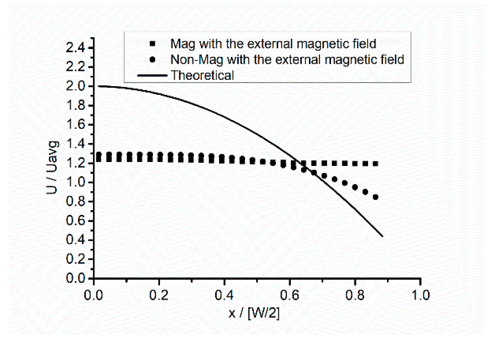
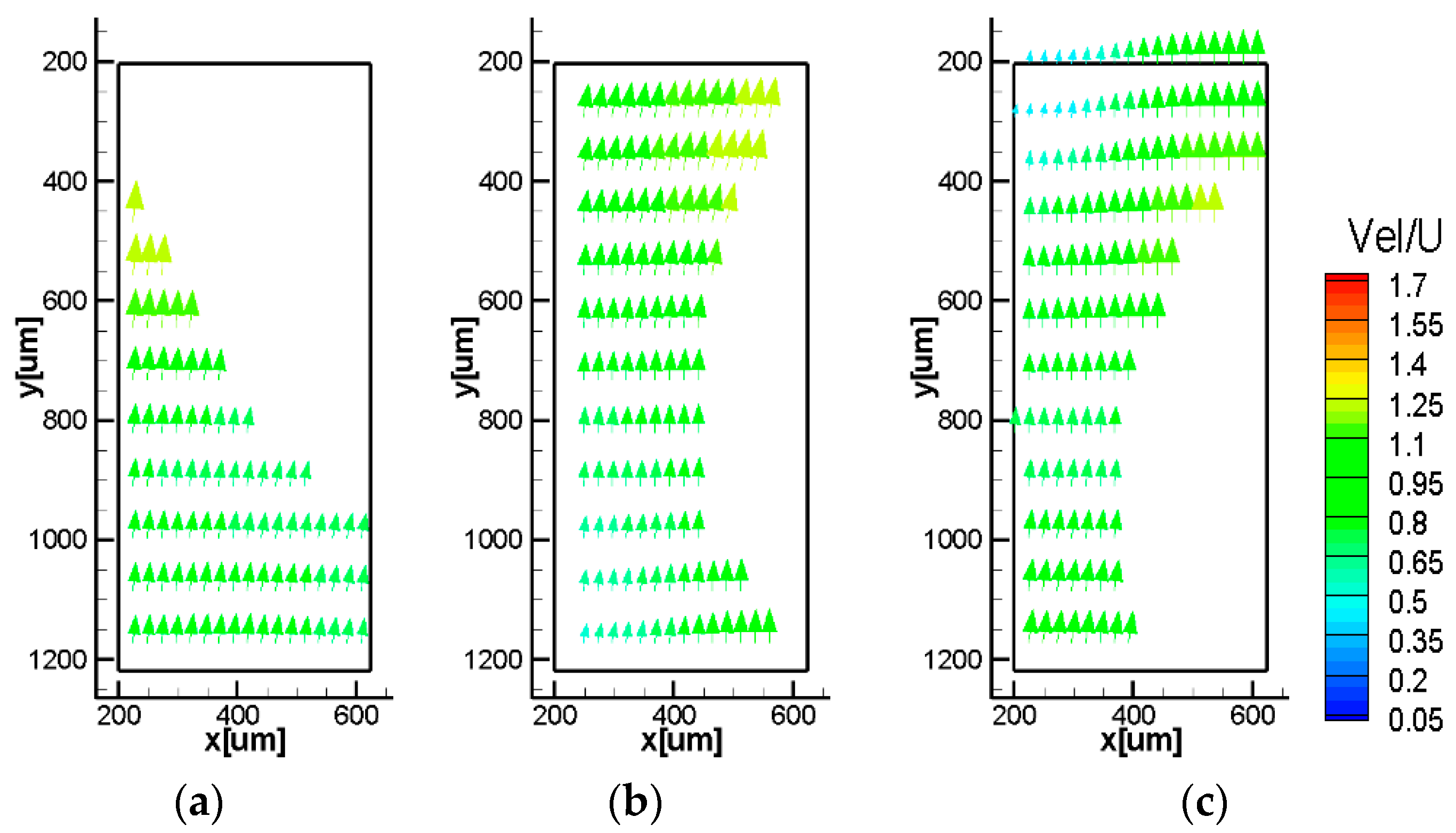
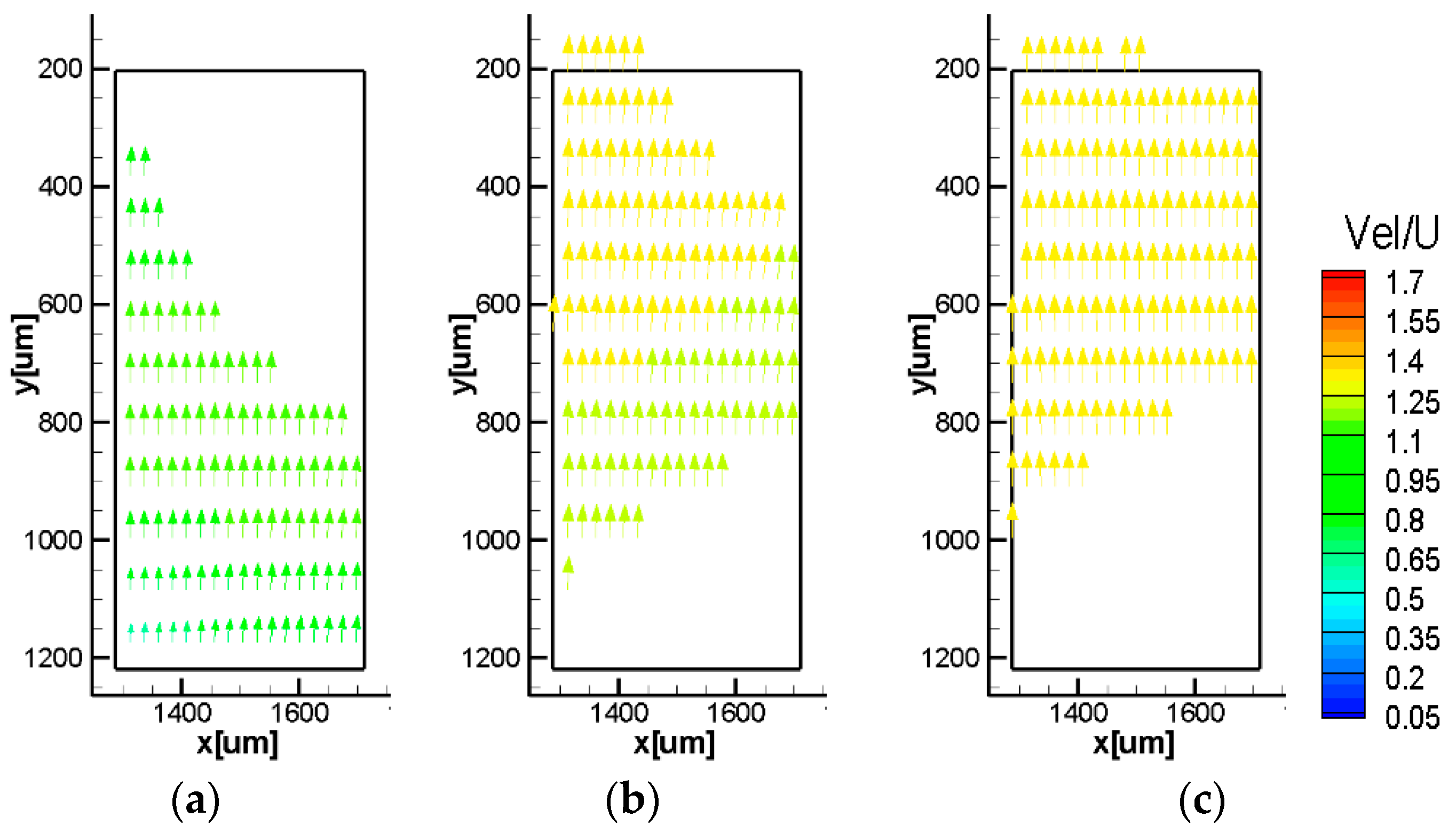
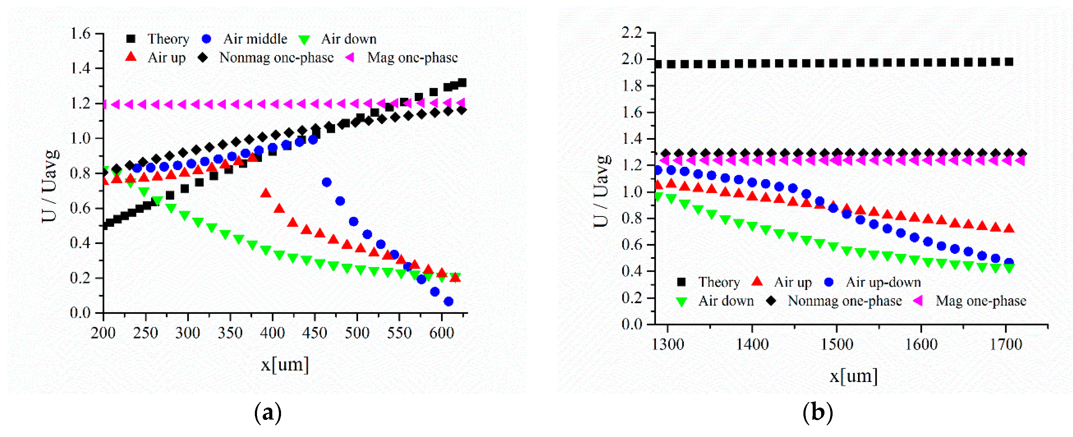
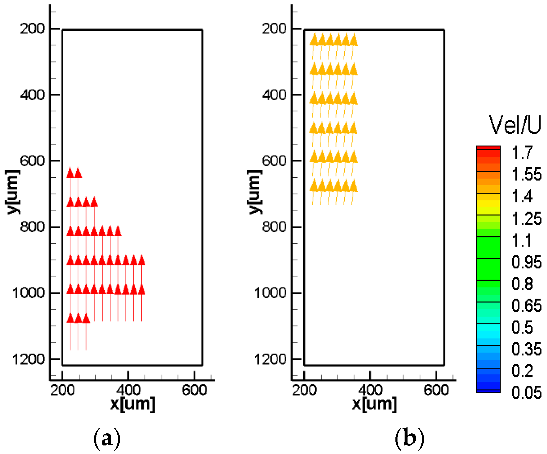
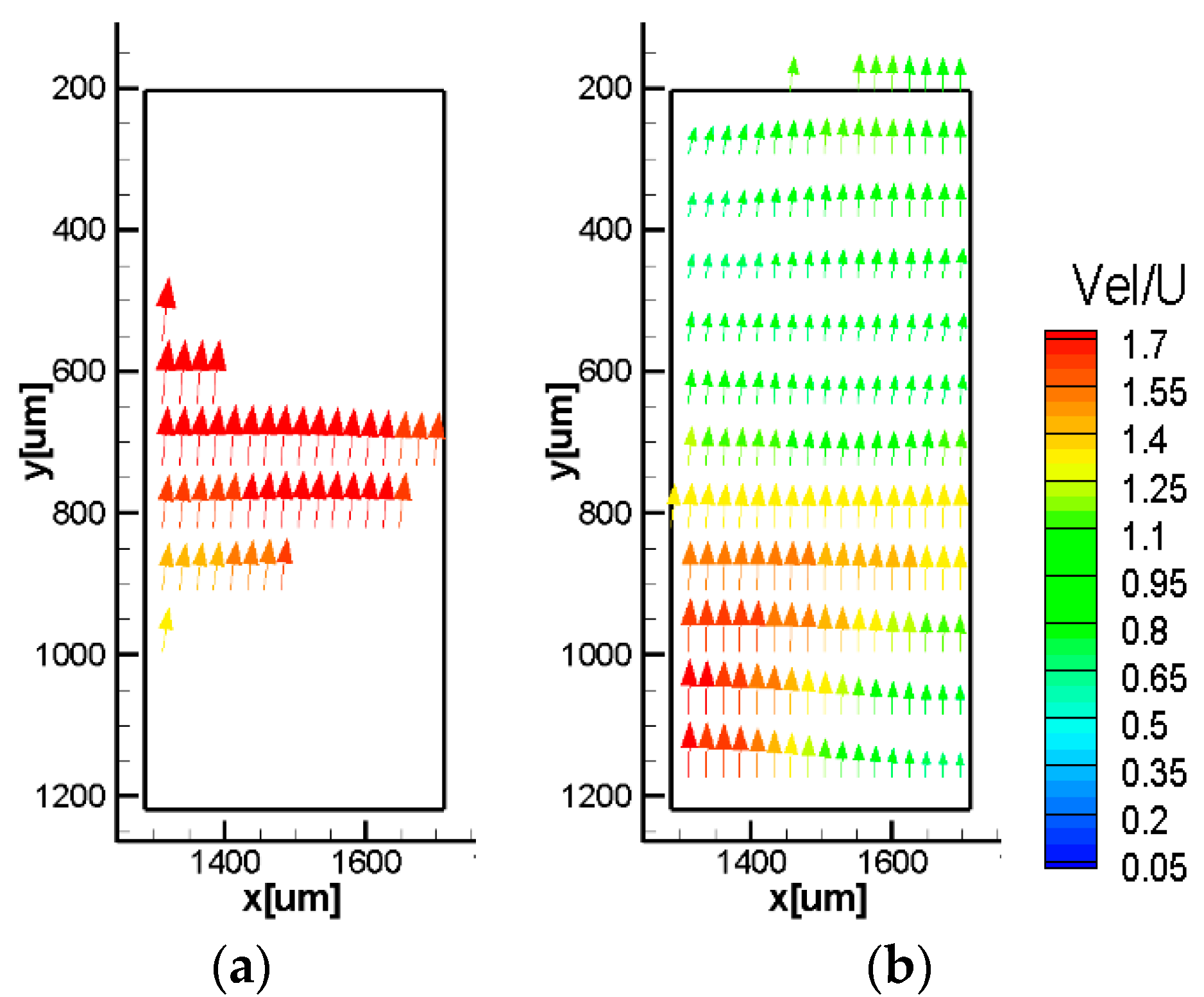
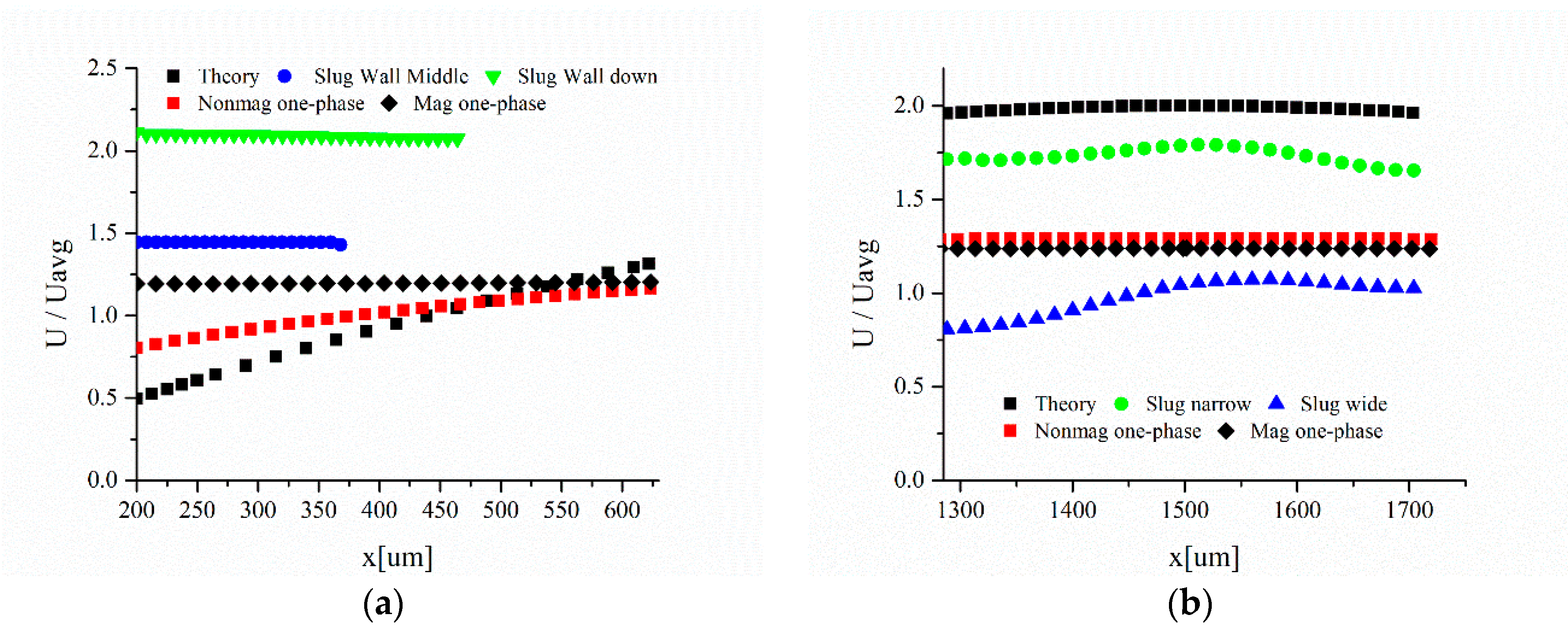
3.2.1. Velocity Fields

Figure 9 shows the velocity field of magnetic particles measured at 200 μm toward the center from the wall. The calculation area was approximately H 1000 × W 424 μm². Voids in the velocity field made up the areas where bubbles were present. Figure 9a shows magnetic particles present below the N₂ bubbles. The velocity of the magnetic particles becomes faster as the gap between the bubble and the wall becomes narrower, comparing with Figure 9b,c. The cross section becomes smaller, and the velocity increases because the velocity of a magnetic particle is greater than the N₂ velocity. In Figure 9b, magnetic particles and bubbles are shown in the middle. The velocities exhibited at the center and bottom of the N₂ bubbles are lower than the velocity at the top. In Figure 9c, magnetic particles are shown above the N₂ bubbles. Thus, the flow phenomenon changes completely depending on the size of the gap between the wall and the N₂ bubble. This phenomenon seems to be the result of the magnetic particles’ velocity being greater than the N₂ velocity, which causes the bubbles to act as resistance.

Figure 10 shows the velocity fields at the center of the solenoid nozzle. The center of the nozzle was located 1500 μm away from the wall. The calculated area was approximately 212 μm from either side of the center. In Figure 10a, the magnetic particles are shown below the bubble. In Figure 10b, magnetic particles are present between the bubbles which are located above and below. In Figure 10c, the magnetic particles are above the bubble. Higher velocities were measured in instances where magnetic particles were present above the bubble than when they were present below the bubble. Since the magnetic particles flow in alignment with the external magnetic force, a generally uniform flow field was measured.

Figure 11 shows graphs comparing the theoretical, single-phase nonmagnetic particle, single-phase magnetic particle, and two-phase experimental velocities near the wall and at the center. In Figure 11a, the red and blue profiles of the discontinuous points indicate the boundary of the bubble. These results show that the velocity at the bubble boundary is lower than that far from the bubble. Near to the wall, the velocity of the two-phase flow was found to be lower than those of the single-phase nonmagnetic and magnetic particle flow but higher than the theoretical velocity. At the center, all cases were affected by the external magnetic field, and lower velocities than the theoretical velocity were measured.

Figure 12a shows the velocity field near the wall below the slug. Figure 12b shows the velocity field between the slug and the wall. In contrast to the phenomenon in the bubbly flow, high velocity near the wall was measured in the slug flow despite the external magnetic force acting as an opposing force.

The overall velocity of the magnetic particles appears to have increased because of the high N₂ velocity. Figure 13a shows the velocity field of a narrow place where the gap between slugs was 200 μm. Figure 13b shows the velocity field of an area with a gap of at least 1000 μm between slugs. While the theoretical velocity was 2 and the bubbly flow velocity was approximately 1, the velocity of an area with a narrow slug gap was measured to be over 1.5. An unstable flow phenomenon with a velocity distribution of 0.7–1.5 was found in an area with a wide gap between slugs. The reason for this phenomenon could be that even at the center where the external magnetic force is strong, if the gap between slugs is narrow, the slug velocity exhibits more action on the magnetic particles than the external magnetic force does, drawing the magnetic particles closer. In a wide gap between slugs, the slugs have a partial effect, and the magnetic particle shows a nonuniform velocity field.

Figure 14 shows graphs comparing the theoretical, single-phase nonmagnetic particle, single-phase magnetic particle, and two-phase experimental velocities near the wall and at the center. Near the wall, the velocity of the slug flow is higher than the other velocities. The velocity between under the slug and the wall is higher than that between the wall and the slug. A lower velocity was measured at the center due to the external magnetic force effect. At the narrow gap between the slugs, a high velocity of approximately 1.7 was measured, but at the wide gap, a low velocity of approximately 0.9 was measured.

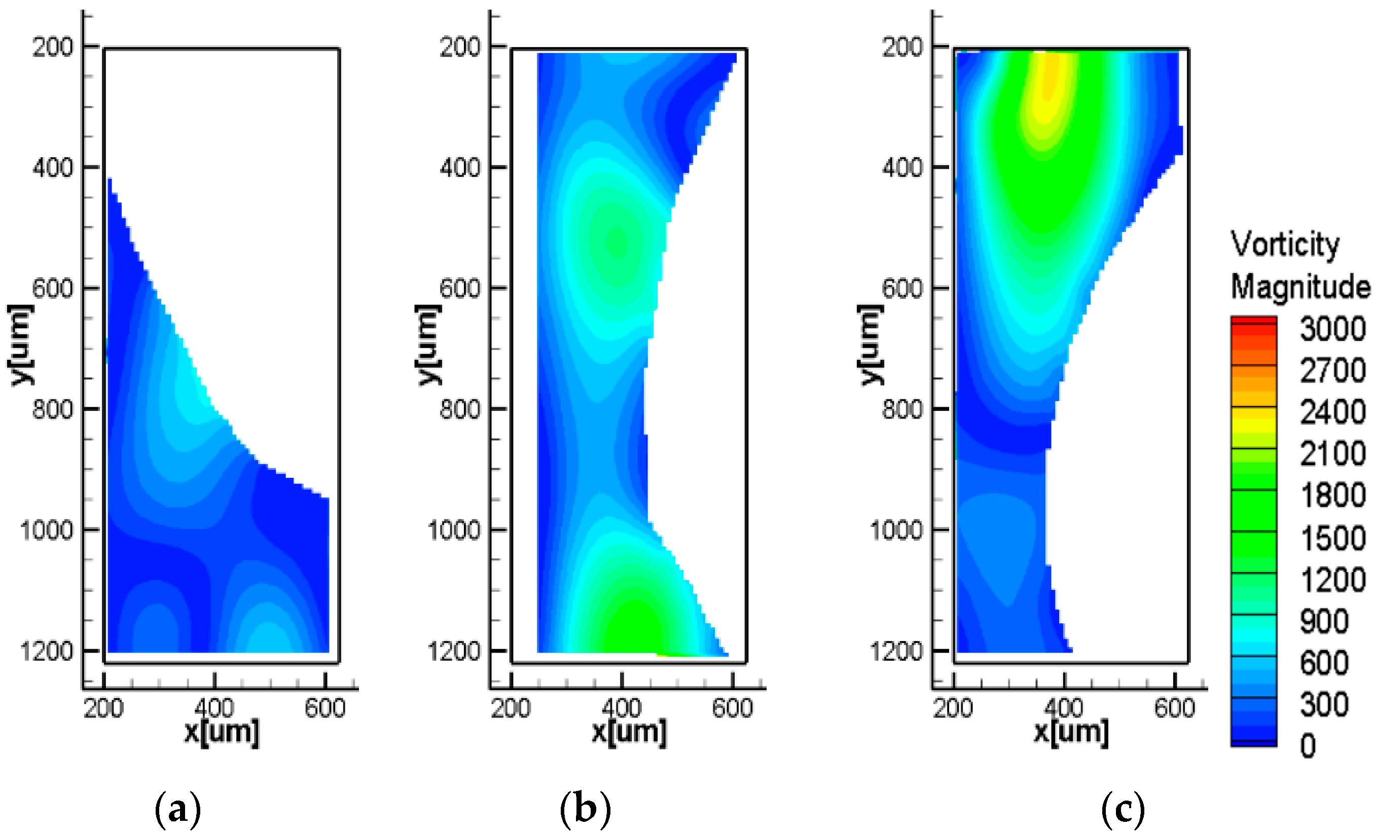
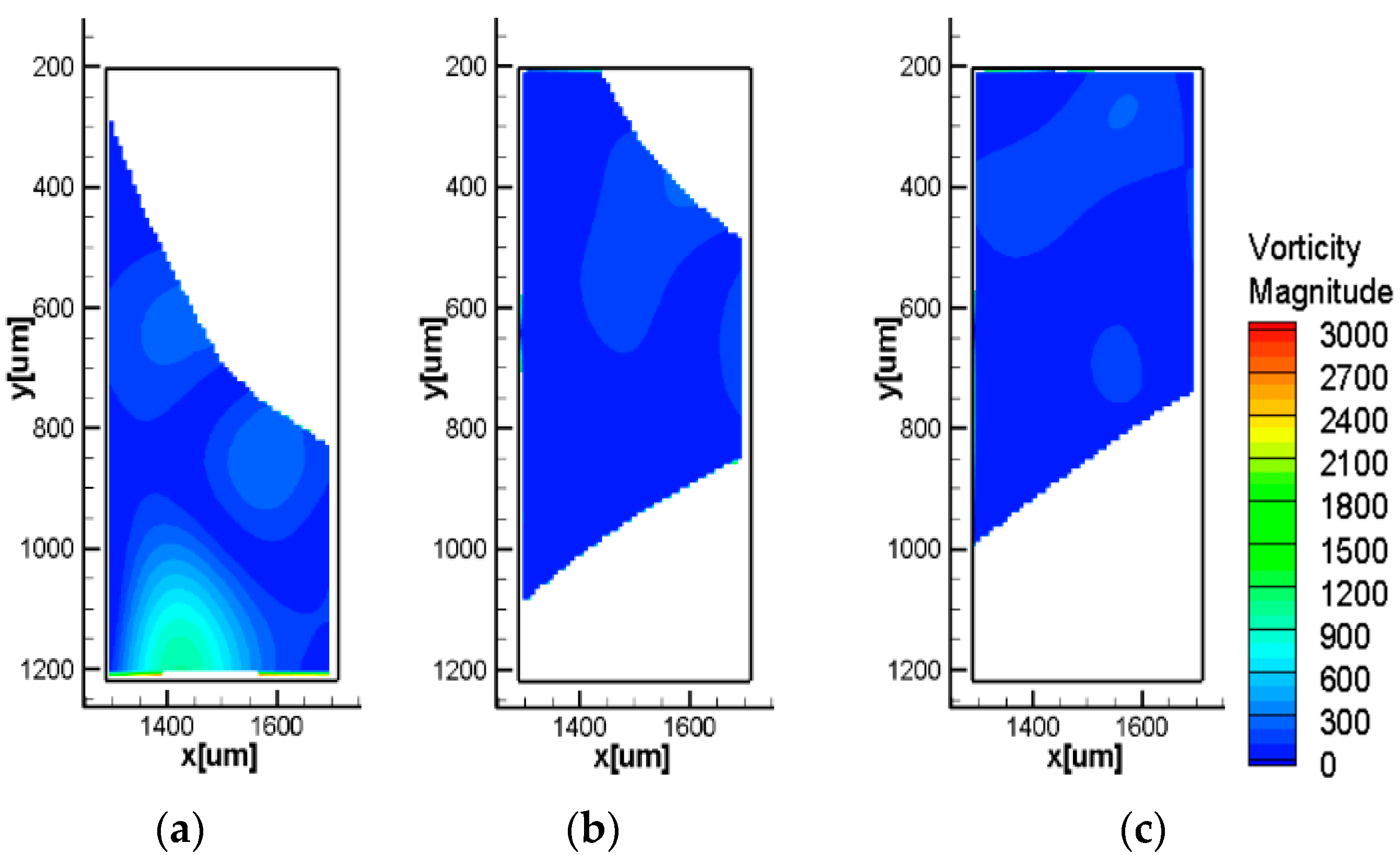
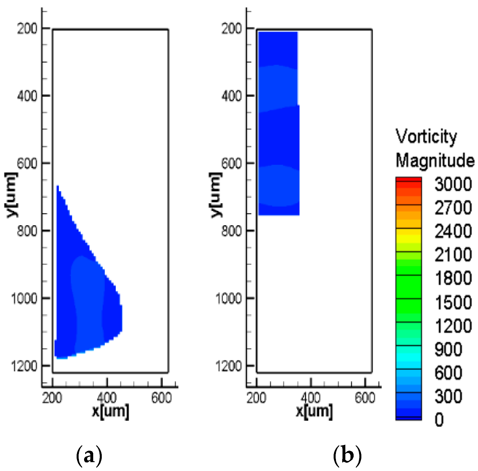
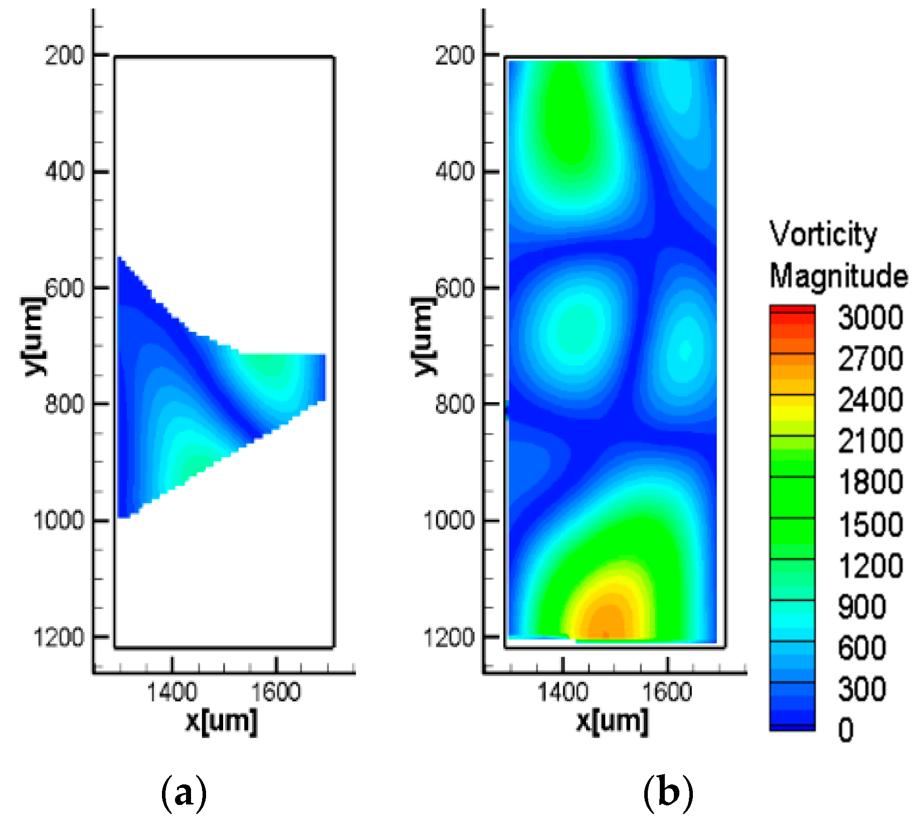
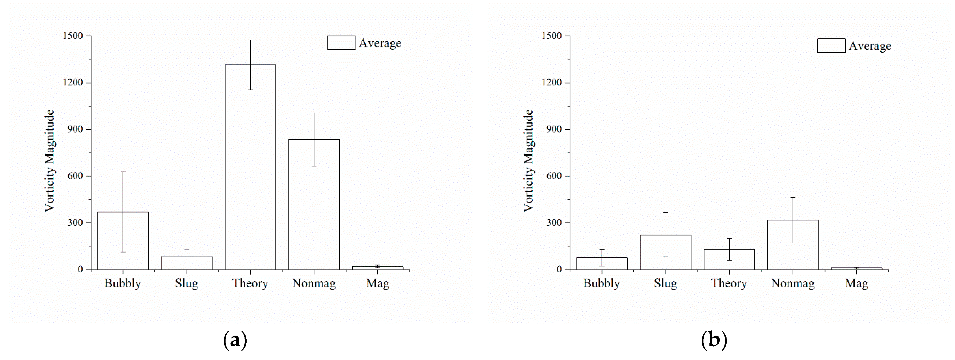
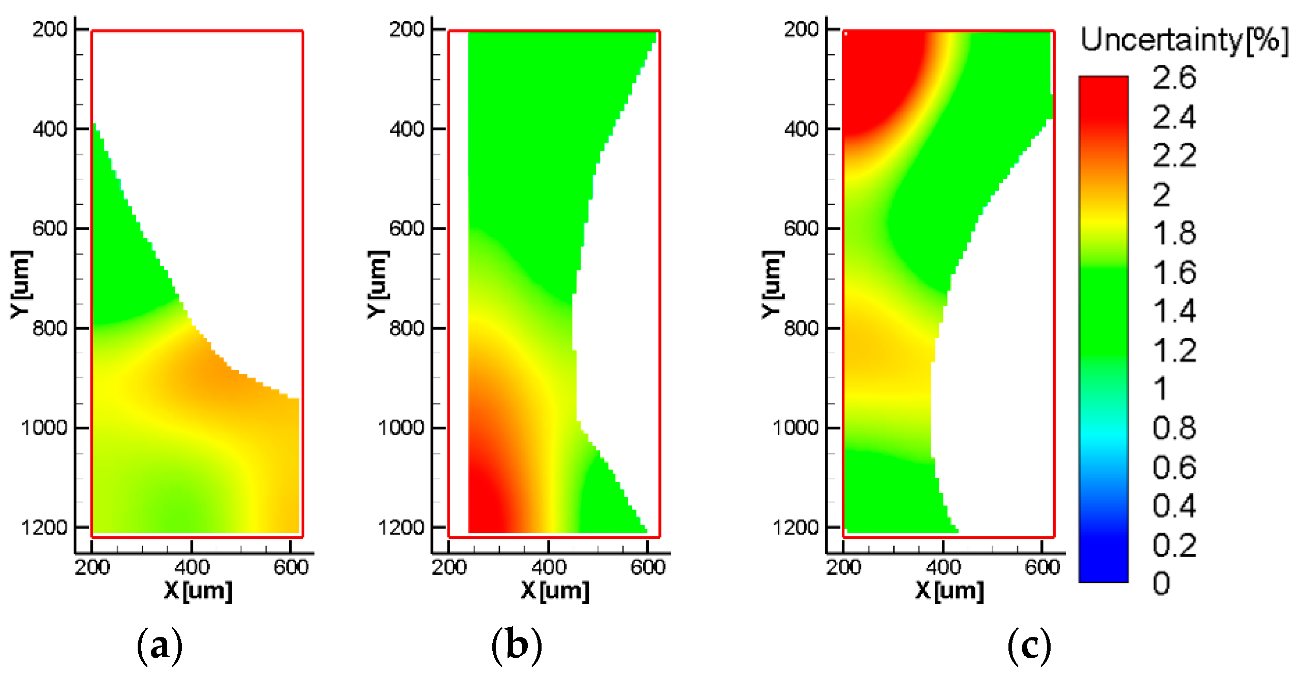
3.2.2. Vorticity Fields

Figure 15 shows the vorticity field near the wall, while Figure 16 shows the vorticity field at the center. In each figure, the bubbles are positioned the same as in the velocity fields. The magnetic particle flow receives a very small effect from the wall due to the external magnetic force.

Figure 17a shows the vorticity field near the wall below the slug; Figure 17b shows the vorticity field between the slug and the wall; Figure 18a shows the vorticity field of the area at the center with a narrow gap between the slugs; and Figure 18b shows the vorticity field of the area at the center with a wide gap between slugs. Near the wall, the slug vorticity is shown to be lower than the bubbly vorticity. The vorticity at the center is higher than that near the wall. These results are due to the high difference in velocity between the N₂ and water.

Figure 19a shows the average vorticity near the wall, while Figure 19b shows the average vorticity at the center, taking in the calculated area compared to the bubbly area, the slug, the theoretical result, and the single-phase nonmagnetic particle and magnetic particle vorticity. Near the wall, the bubbly flow, slug flow, and single-phase magnetic particle values were found to be 44.2%, 10% and 2.3%, respectively, compared to the single-phase nonmagnetic particle value. The experimental results of the two-phase and single-phase magnetic particles near the wall had lower values than the theoretical and the single-phase nonmagnetic results. Since the cross section of the flow field width was uniform, the slug flow had a lower vorticity than the bubbly flow, even when the N₂ velocity was high.

At the center, the bubbly flow, slug flow, and single-phase magnetic particle had values of 23.8%, 70.4% and 3.3%, respectively, compared to the single-phase nonmagnetic particle value. The experimental results of the bubbly flow and the single-phase magnetic particle showed lower values than the theoretical and the nonmagnetic results. The vorticity of the slug flow was higher than that of the bubbly flow. However, all of the values at the center were lower than those near the wall. According to these results, the vorticity was reduced by the external magnetic field near the wall and at the center.

Figure 20, Figure 21 and Figure 22 are velocity uncertainty fields. The uncertainty of the measured velocity was analyzed using the method developed by Holman [36]. The uncertainty of the velocity was estimated to be up to 2.6%.

4. Conclusions

In this study, it was shown that our unique LIF-PIV setup can successfully measure the velocity of magnetic particles under the influence of an external magnetic field in two-phase flow.

For the bubbly flow, the velocity near the wall was found to be similar to that of the flow at the center. The flow phenomenon differed depending on the size of the gap between the wall and the bubble. When this gap was less than 400 μm, an increasingly higher velocity was measured for narrower gaps between the bubble and the wall. For gaps larger than 400 μm, no such phenomenon was present. This shows that for narrow gaps, the velocity of the magnetic particles was higher than that of the bubble. The bubble played the role of an obstacle inside the pipe.

For the slug flow, the flow near the wall was measured to be higher than the flow at the center. Furthermore, the velocity decreased for wider slug gaps, and it increased for narrower slug gaps. The reason for this phenomenon could be that the slug velocity had a greater effect on the magnetic particles than did the external magnetic force.

To determine the degree of the nonrotational property, it was compared to theoretical flow and to single-phase nonmagnetic and magnetic particle vorticities. In the vorticity field, due to the effect of the external magnetic field, the vorticities of the bubbly flow and slug flow were lower than that of the single-phase nonmagnetic particle flow near the wall. At the center, the bubbly flow showed a lower vorticity than did the theoretical and single-phase nonmagnetic particle flows. However, the slug flow was higher than the theoretical flow. All of the experimental results were reduced by the presence of an external magnetic field when compared with the single-phase nonmagnetic particle results. These results mean that the ferrofluid was vertically aligned when it passed through the external magnet.

In summary, the characteristics of two-phase flow under the magnetic field were studied using an experimental measurement. The experimental data contributed towards the development of a database that can be used to validate computational fluid dynamics simulations. The research methods proposed in this paper will contribute towards improvements in the design of the solenoid nozzle and the control of ferrofluid.

References

1. Asfer, M.; Prasad Prajapati, A.; Kumar, A.; Kumar Panigrahi, P. Visualization and Motion of Curcumin Loaded Iron Oxide Nanoparticles During Magnetic Drug Targeting. J. Nanotechnol. Eng. Med. 2015, 6, 011004. [Google Scholar] [CrossRef]
2. Hamdipoor, V.; Afzal, M.; Le, T.-A.; Yoon, J. Haptic-Based Manipulation Scheme of Magnetic Nanoparticles in a Multi-Branch Blood Vessel for Targeted Drug Delivery. Micromachines 2018, 9, 14. [Google Scholar] [CrossRef] [PubMed] [Green Version]
3. Bibo, A.; Masana, R.; King, A.; Li, G.; Daqaq, M.F. Electromagnetic ferrofluid-based energy harvester. Phys. Lett. Sect. A Gen. At. Solid State Phys. 2012, 376, 2163–2166. [Google Scholar] [CrossRef]
4. Seol, M.-L.; Jeon, S.-B.; Han, J.-W.; Choi, Y.-K. Ferrofluid-based triboelectric-electromagnetic hybrid generator for sensitive and sustainable vibration energy harvesting. Nano Energy 2017, 31, 233–238. [Google Scholar] [CrossRef]
5. Hartshorne, H.; Backhouse, C.J.; Lee, W.E. Ferrofluid-based microchip pump and valve. Sens. Actuators B Chem. 2004, 99, 592–600. [Google Scholar] [CrossRef]
6. Zeng, J.; Deng, Y.; Vedantam, P.; Tzeng, T.-R.; Xuan, X. Magnetic separation of particles and cells in ferrofluid flow through a straight microchannel using two offset magnets. J. Magn. Magn. Mater. 2013, 346, 118–123. [Google Scholar] [CrossRef]
7. Abdollahi, A.; Salimpour, M.R.; Etesami, N. Experimental analysis of magnetic field effect on the pool boiling heat transfer of a ferrofluid. Appl. Therm. Eng. 2017, 111, 1101–1110. [Google Scholar] [CrossRef]
8. Berensmeier, S. Magnetic particles for the separation and purification of nucleic acids. Appl. Microbiol. Biotechnol. 2006, 73, 495–504. [Google Scholar] [CrossRef]
9. Hejazian, M.; Nguyen, N.-T. A Rapid Magnetofluidic Micromixer Using Diluted Ferrofluid. Micromachines 2017, 8, 37. [Google Scholar] [CrossRef] [Green Version]
10. Yun, H.R.; Lee, D.J.; Youn, J.R.; Song, Y.S. Ferrohydrodynamic energy harvesting based on air droplet movement. Nano Energy 2015, 11, 171–178. [Google Scholar] [CrossRef]
11. Kim, S.-H.; Park, J.-H.; Choi, H.-S.; Lee, S.-H. Power Generation Properties of Flow Nanogenerator With Mixture of Magnetic Nanofluid and Bubbles in Circulating System. IEEE Trans. Magn. 2017, 53, 1–4. [Google Scholar] [CrossRef]
12. Sheikholeslami, M.; Rokni, H.B. Simulation of nanofluid heat transfer in presence of magnetic field: A review. Int. J. Heat Mass Transf. 2017, 115, 1203–1233. [Google Scholar] [CrossRef]
13. El-Amin, M.F.; Khaled, U.; Beroual, A. Numerical study of the magnetic field effect on ferromagnetic fluid flow and heat transfer in a square porous cavity. Energies 2018, 11, 3235. [Google Scholar] [CrossRef] [Green Version]
14. Sheikholeslami, M.; Barzegar Gerdroodbary, M.; Mousavi, S.V.; Ganji, D.D.; Moradi, R. Heat transfer enhancement of ferrofluid inside an 90° elbow channel by non-uniform magnetic field. J. Magn. Magn. Mater. 2018, 460, 302–311. [Google Scholar] [CrossRef]
15. Zare, R.N. My Life with LIF: A Personal Account of Developing Laser-Induced Fluorescence. Annu. Rev. Anal. Chem. 2012, 5, 1–14. [Google Scholar] [CrossRef] [Green Version]
16. Lobanov, P.; Pakhomov, M.; Terekhov, V. Experimental and Numerical Study of the Flow and Heat Transfer in a Bubbly Turbulent Flow in a Pipe with Sudden Expansion. Energies 2019, 12, 2735. [Google Scholar] [CrossRef] [Green Version]
17. Peng, J.; Cao, Z.; Yu, X.; Yu, Y.; Chang, G.; Wang, Z. Investigation of Flame Evolution in Heavy Oil Boiler Bench Using High-Speed Planar Laser-Induced Fluorescence Imaging. Appl. Sci. 2018, 8, 1691. [Google Scholar] [CrossRef] [Green Version]
18. Murgan, I.; Bunea, F.; Ciocan, G.D. Experimental PIV and LIF characterization of a bubble column flow. Flow Meas. Instrum. 2017, 54, 224–235. [Google Scholar] [CrossRef]
19. Siddiqui, M.I.; Munir, S.; Heikal, M.R.; de Sercey, G.; Aziz, A.R.A.; Dass, S.C. Simultaneous velocity measurements and the coupling effect of the liquid and gas phases in slug flow using PIV-LIF technique. J. Vis. 2016, 19, 103–114. [Google Scholar] [CrossRef] [Green Version]
20. Petrosky, B.J.; Lowe, K.T.; Danehy, P.M.; Wohl, C.J.; Tiemsin, P.I. Improvements in laser flare removal for particle image velocimetry using fluorescent dye-doped particles. Meas. Sci. Technol. 2015, 26, 115303. [Google Scholar] [CrossRef]
21. Xiaodong, R.; Feng, W.; Yamamoto, F. PIV measurements for gas flow under gradient magnetic fields. Acta Mech. Sin. 2004, 20, 591–596. [Google Scholar] [CrossRef]
22. Takeuchi, J.; Satake, S.; Kunugi, T.; Yokomine, T.; Morley, N.B.; Abdou, M.A. Development of PIV Technique under Magnetic Fields and Measurement of Turbulent Pipe Flow of Flibe Simulant Fluid. Fusion Sci. Technol. 2007, 52, 860–864. [Google Scholar] [CrossRef]
23. Ali, J.; Kim, H.; Cheang, U.K.; Kim, M.J. Micro-PIV measurements of flows induced by rotating microparticles near a boundary. Microfluid. Nanofluidics 2016, 20, 131. [Google Scholar] [CrossRef]
24. Gilard, V.; Gillon, P.; Blanchard, J.-N.; Sarh, B. Influence of a Horizontal Magnetic Field on a Co-Flow Methane/Air Diffusion Flame. Combust. Sci. Technol. 2008, 180, 1920–1935. [Google Scholar] [CrossRef]
25. Munhoz, D.S.; Bityurin, V.A.; Zavershinskii, I.P.; Klimov, A.I.; Moralev, I.A.; Kazanskii, P.N.; Molevich, N.E.; Polyakov, L.B.; Porfir’ev, D.P.; Sugak, S.S.; et al. Air flow control around a cylindrical model induced by a rotating electric arc discharge in an external magnetic field. J. Phys. Conf. Ser. 2019, 1394, 012008. [Google Scholar] [CrossRef]
26. Tan, L.; Ali, J.; Cheang, U.K.; Shi, X.; Kim, D.; Kim, M.J. µ-PIV Measurements of Flows Generated by Photolithography-Fabricated Achiral Microswimmers. Micromachines 2019, 10, 865. [Google Scholar] [CrossRef] [Green Version]
27. Yang, J.; Park, J.; Lee, J.; Cha, B.; Song, Y.; Yoon, H.G.; Huh, Y.M.; Haam, S. Motions of magnetic nanosphere under the magnetic field in the rectangular microchannel. J. Magn. Magn. Mater. 2007, 317, 34–40. [Google Scholar] [CrossRef]
28. Takeuchi, J.; Satake, S.; Morley, N.B.; Kunugi, T.; Yokomine, T.; Abdou, M.A. Experimental study of MHD effects on turbulent flow of Flibe simulant fluid in circular pipe. Fusion Eng. Des. 2008, 83, 1082–1086. [Google Scholar] [CrossRef]
29. Aminfar, H.; Mohammadpourfard, M.; Mohseni, F. Two-phase mixture model simulation of the hydro-thermal behavior of an electrical conductive ferrofluid in the presence of magnetic fields. J. Magn. Magn. Mater. 2012, 324, 830–842. [Google Scholar] [CrossRef]
30. König, J.; Neumann, M.; Mühlenhoff, S.; Tschulik, K.; Albrecht, T.; Eckert, K.; Uhlemann, M.; Weier, T.; Büttner, L.; Czarske, J. Optical velocity measurements of electrolytic boundary layer flows influenced by magnetic fields. Eur. Phys. J. Spec. Top. 2013, 220, 79–89. [Google Scholar] [CrossRef]
31. Hangi, M.; Bahiraei, M.; Rahbari, A. Forced convection of a temperature-sensitive ferrofluid in presence of magnetic field of electrical current-carrying wire: A two-phase approach. Adv. Powder Technol. 2018, 29, 2168–2175. [Google Scholar] [CrossRef]
32. Shahsavar, A.; Ansarian, R.; Bahiraei, M. Effect of line dipole magnetic field on entropy generation of Mn-Zn ferrite ferrofluid flowing through a minichannel using two-phase mixture model. Powder Technol. 2018, 340, 370–379. [Google Scholar] [CrossRef]
33. Characteristics of sliding bubble in aqueous electrolyte: In presence of an external magnetic field. Colloids Surf. A Physicochem. Eng. Asp. 2018, 538, 404–416. [CrossRef]
34. Westergaard, C.H.; Buchhave, P. PIV: Comparison of three autocorrelation techniques. In Proceedings of the SPIE 205—Fifth International Conference on Laser Anemometry: Advances and Applications, Veldhoven, The Netherlands, 23–27 August 1993; pp. 535–541. [Google Scholar] [CrossRef]
35. Keane, R.D.; Adrian, R.J. Optimization of particle image velocimeters. In Proceedings of the SPIE 1404—ICALEO’89: Optical Methods in Flow and Particle Diagnostics, Orlando, FL, USA, 10–25 October 1989; pp. 139–159. [Google Scholar] [CrossRef]
36. Holman, J.P. Experimental Methods for Engineering, 5th ed.; McGraw-Hill: Singapore, 1989. [Google Scholar]
Figure 1. Schematic of the Organic Inductive Cycle and the solenoid nozzle with the external magnet.
Applsci 10 03976 g001
Figure 2. Schematic of (a) the two-phase vertical flow setup and (b) the solenoid nozzle setup. (c) Experimental setup of the two-phase flow.
Applsci 10 03976 g002
Figure 3. (a) The solenoid nozzle with coils. (b) Cross section of the solenoid nozzle.
Applsci 10 03976 g003
Figure 4. Magnetic flux density field and profile. The red box indicates the profile position.
Applsci 10 03976 g004
Figure 5. Schematics of (a) the laser-induced fluorescence LIF-PIV setup, (b) the beam path setup, (c) the beam reducing setup, and (d) the particle detection setup.
Applsci 10 03976 g005
Figure 6. The timing chart for the LIF-PIV.
Applsci 10 03976 g006
Figure 7. A raw image of the bubbly flow. Captured in the Davis PIV analysis program.
Applsci 10 03976 g007
Figure 8. Velocity profiles for magnetic and nonmagnetic particles and from theoretical calculations.
Applsci 10 03976 g008
Figure 9. Velocity fields of bubbly flow near the wall. The N2 is located (a) above, (b) middle, (c) below.
Applsci 10 03976 g009
Figure 10. Velocity fields of bubbly flow at the center. The N2 is located (a) above, (b) above and below, (c) below.
Applsci 10 03976 g010
Figure 11. Comparison of the average velocity profiles of the bubbly flow (a) near the wall and (b) at the center.
Applsci 10 03976 g011
Figure 12. Velocity fields of the slug flow near the wall. The slug is located (a) above (b) beside.
Applsci 10 03976 g012
Figure 13. Velocity fields of slug flow at the center. The slug is located with a (a) narrow (b) wide gap.
Applsci 10 03976 g013
Figure 14. A comparison of velocity profiles of the slug flow (a) near the wall and (b) at the center.
Applsci 10 03976 g014
Figure 15. Vorticity fields of bubbly flow near the wall. The N2 is located (a) above, (b) middle, (c) below.
Applsci 10 03976 g015
Figure 16. Vorticity fields of bubbly flow at the center. The N2 is located (a) above, (b) above and below, (c) below.
Applsci 10 03976 g016
Figure 17. Vorticity fields of slug flow near the wall. The slug is located (a) above, (b) beside.
Applsci 10 03976 g017
Figure 18. Vorticity fields of slug flow at the center. The slug is located with a (a) narrow (b) wide gap.
Applsci 10 03976 g018
Figure 19. A comparison of the bubbly flow, slug flow, theoretical, and single-phase nonmagnetic and magnetic vorticity values (a) near the wall and (b) at the center.
Applsci 10 03976 g019
Figure 20. Uncertainty fields of the bubbly flow near the wall. The N2 is located (a) above, (b) middle, (c) below.
Applsci 10 03976 g020
Figure 21. Uncertainty fields of the slug flow near the wall. The N2 is located (a) above, (b) middle, (c) below.
Applsci 10 03976 g021
Figure 22. Uncertainty fields (a) near the wall, slug above; (b) near the wall, slug beside; (c) at the center, with a narrow slug gap; and (d) at the center, with a wide slug gap.
Applsci 10 03976 g022