Robust Control for Active Suspension of Hub-Driven Electric Vehicles Subject to in-Wheel Motor Magnetic Force Oscillation

Featured Application

The aim of this study is to provide an accurate model reference for the analysis of vibration characteristics of hub-driven electric vehicles with permanent magnet synchronous motors (PMSM) and the optimization, control and improvement of its vibration performance. It can be applied to intelligent suspension designof hub-driven electric vehicles.

Abstract

In this paper, after investigating the coupling effect in a permanent magnet synchronous in-wheel motor, a robust control method for active suspension of hub-driven electric vehicles (EVs) to enhance the performance of the in-wheel motor and the vehicle is proposed. Based on the electric vehicle model addressing the coupling effect between the electromagnetic excitation of the permanent magnet synchronous motor (PMSM) and the transient dynamics in EVs, the influence of the coupling effect on the motor and the vehicle performance is analyzed. The results reflect that the coupling effect in in-wheel motors intensifies the magnetic force oscillation, aggravates the eccentricity of the rotor, deteriorates the motor operation performance, and worsens the ride comfort. To suppress the magnetic force oscillation in motor and enhance the vehicle comfort, the active suspension system considering five aspects of suspension performance is introduced. Simultaneously, on the basis of Lyapunov stability theory, a reliable robust H_ꝏ controller considering model uncertainties, actuator failure and electromagnetic force interference is designed. The simulation results reflect that the robust H_ꝏ feedback controller can not only achieve better ride comfort, but also restrain the coupling effect in the motor. Meanwhile the other requirements such as the road holding capability, the actuator limitation, and the suspension deflection are also maintained. The proposed robust control method demonstrates a potential application in the practice of EV control.

1. Introduction

Due to the aggravation of environmental pollution and the energy crisis, automotive products are required to be energy-saving, highly efficient, and environmentally-friendly [1,2,3]. Compared with traditional diesel locomotives, electric vehicles (EVs) which have several advantages such as no CO₂ emission and energy efficiency have caught widespread attention in recent years [4,5]. The propulsion configurations of EVs can be classified as a distributed motor driven layout and a centralized driven layout. Compared with centralized driven layout EVs, in-wheel motor (IWM) propelling EVs, as the distributed propulsion system, enjoy various additional structure and control merits [6,7]. As in the IWM the brake and the reducer are integrated into the rim, the mechanical transmission system of hub-driven EVs is simpler and more efficient. Moreover, by controlling the torque of each electric motor precisely and independently, hub-driven EVs have played a significant role in enhancing the performance of existing vehicle stability/motion control systems, such as electronic stability control systems (ESC) and traction control systems (TCS) [8]. However, the development of hub-driven EVs has introduced some new technical problems. The integration of the driving system into the rim leads to an increase in the unsprung mass, which deteriorates road handling capacities and the ride comfort of vehicles [9,10]. What is more, the road surface roughness excitation and the coupling effect in IWM make the magnet gap deformed. The deformed magnet gap then leads to magnetic force oscillation which is a critical vibration source for vehicle dynamics [11,12].

In the past decades, some passive and active methods, such as optimization of the vibration isolator, redesign of the IWM, and active control for suspension systems, have been adopted to suppress magnetic force oscillation and improve the ride comfort. However, there are some deficiencies which remain to be solved. Luo et al. [12] proposed a novel IWM topology scheme and studied the coupling effect of the IWM system. By mounting rubber bushings in the IWM device, the vibration energy from the road surface was absorbed and the deformation of magnet gap was restricted. However, the life of the rubber bushing was short due to the severe operating environment of the IWM, making it difficult for practical use. Moreover, due to neglect of the permanent magnet brushless direct current (PMBDC) motor model which could provide the phase current for calculating the unbalanced electromagnetic force (UEF), the established coupling model was simple and inaccurate. The transient characteristics of electromechanical coupling effect cannot be effectively studied under vehicle running conditions. Zhao et al. [13] designed the motor mount, making the motor mass as dynamic vibration absorber. The results show that the ride comfort was improved. However, there was a distinct axis relative displacement between the rotor and the stator, prompting magnet gap deformed and magnetic force oscillation. The active suspension control methods have been proposed to suppress the magnetic force oscillation. Nevertheless, the majority of the active suspension system of hub-driven EVs are based on switched reluctance in-wheel driven motors [14,15] or neglect the negative electromagnetic coupling effect in IWM [16,17,18,19]. Different from switched reluctance motors (SRM), the magnetic field in permanent magnet synchronous motors (PMSM) is provided by permanent magnets. Consequently, as a permanent magnet synchronous IWM, more complex multi-field coupling effects need to be studied to enhance the ride comfort of EVs. In brief, it is meaningful to suppress magnetic force oscillation and improve the ride comfort. However, for the PMSM, the passive methods to suppress magnetic force oscillation have some defects and the active methods are rarely studied. Furthermore, the electromagnetic coupling model of hub-driven electric vehicle based on PMSM that has been established by Luo is inaccurate [12]. It is necessary to establish the complete electromagnetic coupling model, investigate the coupling mechanism of PMSM and study the active control methods for the suspension system of hub-driven electric vehicle to solve the negative coupling effect of the PMSM.

Besides, failures of electrical components, sensors, and the actuator are fairly common to active suspension systems, which will lead to a series of problems, such as system instability, performance degradation, and even disaster traffic accidents. Therefore, it is of great significance to design the active suspension considering actuator failures. Choi et al. [20] proposed a robust controller for a semi-active suspension system with actuator saturation. The vehicle vibration attenuation problem under two cases was addressed, namely, without actuator fault and with base oil leakage in MR damper. Liu et al. [21] proposed a new adaptive fault tolerant control scheme by employing adaptive feed-back stepping technique which ensured the boundedness in probability of the considered systems. Alain et al. [22] presented an application of a diagnosis and a fault-tolerant control method for an active suspension system. This method could improve the vehicle performance in the presence of road disturbances by identifying an actuator fault and reconfiguring the controller. In the literature [23,24,25], the fault-tolerant control was proposed for an active suspension system with an actuator fault. The results showed that the control effects of the active suspension system deteriorated without considering the actuator failure. Similarly, the control effects will be unsatisfactory if the model parameter uncertainties are neglected. In the literature [26,27,28], the robust control was proposed for vehicle active suspensions. The comparative simulations presented the availability of the designed controllers considering the model uncertainties. In addition, some other control methods were also proposed to suppress disturbance and obtain the better performance of the system, such as u-synthesis [29], neural network method [30], mixed H_ꝏ/H₂ [31], slide-mode control [32,33,34,35,36], adaptive control [37], and nonlinear control [38,39]. However, most of the control strategies are proposed for conventional vehicles and rarely for PMSM-driven EVs. From the existing studies, the issues of active suspension systems associated with actuator fault tolerance, model parameter uncertainties, and coupling effect in IWM based on PMSM have not been well studied in previous research.

This paper focuses on the coupling effect in permanent magnet synchronous IWM and the robust control for active suspension of hub-driven EVs. The challenges and technical contributions are summarized as follows: (1) unlike studies in Ref. [11,12], in which the established electromechanical coupling model was simple and inaccurate, in this paper, according to the electromagnetic field theory, the complete electromechanical coupling model of the hub-driven EVs composed of four sub-models is established. The transient characteristics of electromechanical coupling effect can be effectively studied under vehicle running conditions; (2) unlike studies in Ref. [15,16,24], in which the authors proposed active suspension controller for the SRM driven electric vehicle, the electric vehicle neglecting the coupling effect or the conventional vehicle, in this study, a multi-objective control is designed for the PMSM driven EV to obtain better ride comfort and restrict coupling effect of in-wheel PMSM. Meanwhile, the other performances such as actuator limitation, small suspension deflection and road holding capability are also maintained; (3) the suspension parameter uncertainties and actuator fault are simultaneously considered and a reliable robust H∞ controller is designed to attenuate the effects caused by the magnetic force oscillation, parameter uncertainties, the actuator fault and road disturbances.

The rest of this paper is organized as follows. In Section 2, the mathematical model of a hub-driven electric vehicle is established and the coupling effect is analyzed. In Section 3, a reliable robust H∞ controller is presented. The simulation results are described in Section 4 and key conclusions are given in Section 5.

2. System Modelling and Problem Formulation

As magnetic force oscillation worsens the performance of EV, the electric vehicle model considering the coupling effect of IWM is established to explore the influence of the coupling effect on vehicle performance and provide a theoretical basis for designing active suspension controller later.

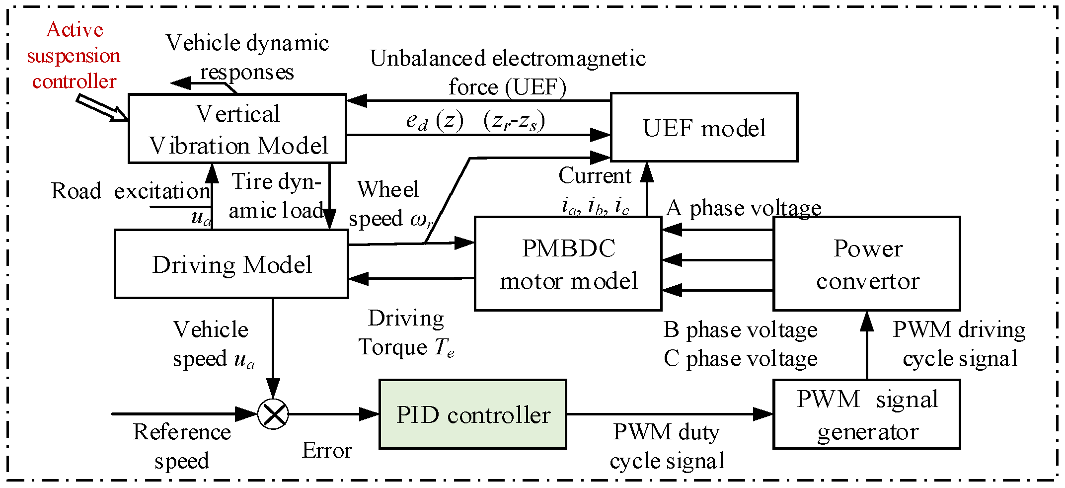
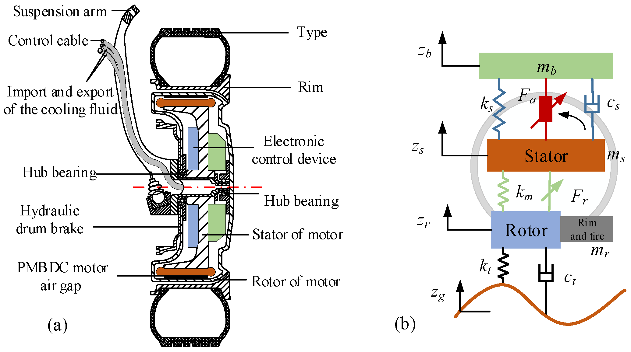
2.1. Hub-Driven Electric Vehicle Modelling

To obtain more precise results, an electric vehicle model considering coupling effect in IWM is developed. It consists of four sub-models: a UEF model, permanent magnet brushless direct current (PMBDC) motor model, driving model and vertical vibration model. The information exchange among them is depicted in Figure 1 and described in detail in following sub-models.

The electric vehicle model consists of two controllers: a PMBDC motor proportional-integral-derivative (PID) controller and an active suspension controller in a vertical vibration model. The active suspension controller is designed to improve the performance of the motor and the vehicle. The PID controller is used to calculate the pulse width modulation (PWM) duty cycle according to the vehicle speed error between the current and the reference. Then, the driving torque of IWM is adjusted based on PWM duty cycle.

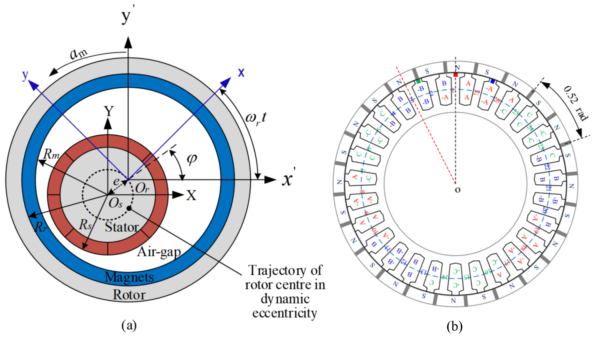
2.1.1. Unbalanced Electromagnetic Force Model

The dynamic vibration in vehicle and UEF (calculated by the UEF model) can evoke a magnet gap deformation which results in magnetic force oscillation as shown in Figure 2a, where O_s and O_r are the geometric center of the stator and the rotor, respectively. In this paper, we are mainly concerned about the rotor eccentricity in the vertical direction. Hence, the uneven magnet gap of IWM is a function of angle a_m and its expression is

$${\delta }_e\left(a_m\right)=\delta -e_d(z)\cos \left(a_m\right)$$

(1)

where e_d (z) denotes relative displacement between the rotor and the stator. It can be provided by vertical vibration model of the EVs with IWMs.

Rotor eccentricity leads to the change of the permeance in magnet gap, and it can be calculated by:

$$\begin{array}{ll}{\lambda }_e& =\frac{u_0}{{\delta }_e\left(a_m\right)}=\frac{u_0}{\delta -e_d(z)\cos \left(a_m\right)}=\frac{u_0}{\delta }\cdot \frac{\delta }{\delta -e_d(z)\cos \left(a_m\right)}\\ & =\lambda \cdot \frac{\delta }{\delta -e_d(z)\cos \left(a_m\right)}=\lambda {\xi }_{\delta }\end{array}$$

(2)

where ξ_δ is the correction coefficient for the permeance. In this study, the 27-slot/24-pole surface PMBDC motor is adopted. The analytical expressions of the radial and the tangential flux density (B_{_pru}(r, a_m, t) and B_{_ptu}(r, a_m, t)) of the slotless field model in the middle of the air gap (r = R_s − g/2) produced by the permanent magnets (PMs) can be given by

$$B_{\_pru}\left(r,a_m,t\right)={\displaystyle \sum _{n=1,3,5...}^{\infty }{K}_B\left(n\right)}\cdot f_{Br}\left(r\right)\cdot \cos [np(a_m-{\omega }_{r}t-{\theta }_0)]$$

(3)

$$B_{\_ptu}\left(r,a_m,t\right)={\displaystyle \sum _{n=1,3,5...}^{\infty }{K}_B\left(n\right)}\cdot f_{Bt}\left(r\right)\cdot \sin [np(a_m-{\omega }_{r}t-{\theta }_0)]$$

(4)

where p denotes the rotor pole-pair number, ɑ_m denotes the angular position, and ω_r denotes angular velocity of the rotor. The parameters of IWM are listed in Appendix A. (The details about the motor can be found in the literature [40,41]).

The winding distribution of the PMBDC motor is shown in Figure 2b. The radial and the tangential flux density (B_{_aru}(r, a_m, t) and B_{_atu}(r, a_m, t)) produced by 3-phase winding of the IWM in the middle of the air gap can be calculated as

$$\begin{array}{ll}{B}_{\_aru}\left(r,a_m,t\right)=& {\displaystyle \sum _{v=1}^{\infty }{B}_{vr}\{I_A(t){\displaystyle \sum _{i=1}^9{s}_{Ai}\cos v\left[a_m-\frac{2\pi }{Q_s}\left(a_{Ai}-1\right)\right]}} + I_B(t){\displaystyle \sum _{i=1}^9{s}_{Bi}\cos v\left[a_m-\frac{2\pi }{Q_s}\left(a_{Bi}-1\right)\right]}\\ & + I_C(t){\displaystyle \sum _{i=1}^9{s}_{Ci}\cos v\left[a_m-\frac{2\pi }{Q_s}\left(a_{Ci}-1\right)\right]}\}\end{array}$$

(5)

$$\begin{array}{ll}{B}_{\_aru}\left(r,a_m,t\right)=& {\displaystyle \sum _{v=1}^{\infty }{B}_{vt}\{I_A(t){\displaystyle \sum _{i=1}^9{s}_{Ai}\cos v\left[a_m-\frac{2\pi }{Q_s}\left(a_{Ai}-1\right)\right]}} + I_B(t){\displaystyle \sum _{i=1}^9{s}_{Bi}\cos v\left[a_m-\frac{2\pi }{Q_s}\left(a_{Bi}-1\right)\right]}\\ & + I_C(t){\displaystyle \sum _{i=1}^9{s}_{Ci}\cos v\left[a_m-\frac{2\pi }{Q_s}\left(a_{Ci}-1\right)\right]}\}\end{array}$$

(6)

where I_A(t), I_B(t), and I_C(t) denote three phase winding current. The detailed derivation of Equations (5) and (6) are referred to in the literature [42,43].

The flux density can be decomposed as the superposition of stator and rotor magnetic fields in the linear case [34]. Thus, the total radial and the tangential flux density (B_{_ru}(r, a_m, t) and B_{_tu}(r, a_m, t)) neglecting the slotting effect can be deduced as

$$B_{\_ru}\left(r,a_m,t\right)=B_{\_pru}\left(r,a_m,t\right)+B_{\_aru}\left(r,a_m,t\right)$$

(7)

$$B_{\_tu}\left(r,a_m,t\right)=B_{\_ptu}\left(r,a_m,t\right)+B_{\_atu}\left(r,a_m,t\right)$$

(8)

It can be found that B_{_ru} and B_{_tu} are functions of phase currents (I_A, I_B, I_C), rotor position ${{\displaystyle \int }}^{}{\omega }_{r}dt$. By introducing the correction coefficient for the permeance ξ_δ, the radial and the tangential flux density (B_{_er}(r, a_m, t) and B_{_et}(r, a_m, t)) considering the influence of rotor eccentricity can be deduced as [44]

$$B_{\_er}\left(r,a_m,t\right)=B_{\_ru}\left(r,a_m,t\right){\lambda }_a{\xi }_{\delta }+B_{\_tu}\left(r,a_m,t\right){\lambda }_b{\xi }_{\delta }$$

(9)

$$B_{\_et}\left(r,a_m,t\right)=B_{\_tu}\left(r,a_m,t\right){\lambda }_a{\xi }_{\delta }-B_{\_ru}\left(r,a_m,t\right){\lambda }_b{\xi }_{\delta }$$

(10)

where λ_a and λ_b denote the influence factors of the stator slotting [45,46]. On the basis of Maxwell magnet stress tensor theory, the radial and tangential magnetic force density distribution (P_er and P_et) under polar coordinate can be calculated [47,48].

$$\begin{array}{l}{P}_{er}\left(r,a_m,t\right)=\frac{1}{2u_0}\left[B_{\_er}{\left(r,a_m,t\right)}^2-B_{\_et}{\left(r,a_m,t\right)}^2\right]\\ P_{et}\left(r,a_m,t\right)=\frac{1}{u_0}\left[B_{\_er}\left(r,a_m,t\right)\cdot B_{\_et}\left(r,a_m,t\right)\right]\end{array}$$

(11)

The magnetic force density distribution in Cartesian coordinate can be obtained according to coordinate transform relationship. Thus, the UMF (F_r) that acts on the stator and the rotor in vertical direction is calculated as

$$F_r=Lr{\displaystyle \underset{0}{\overset{2\pi }{\int }}\left(P_{er}\left(r,a_m,t\right)\cos (a_m)-P_{et}\left(r,a_m,t\right)\sin (a_m)\right)d{a}_m}$$

(12)

where L is the axial gap length of IWM.

2.1.2. PMBDC Motor Model

The PMBDC motor model offers driving torque to promote EV movement and provides phase current for the UEF model to calculate an unbalanced electromagnetic force, as shown in Figure 1. When three-phase winding is star connected, the circuit equations of three windings in phase variables can be expressed as [49]

$$\begin{array}{l}\frac{d}{dt}{I}_A=\frac{1}{3L_s}(2v_{AB}+v_{BC}-3R_s{I}_A+\lambda p{\omega }_r(-2e_A+e_B+e_C))\\ \frac{d}{dt}{I}_B=\frac{1}{3L_s}(-v_{AB}+v_{BC}-3R_s{I}_B+\lambda p{\omega }_r(e_A-2e_B+e_C))\\ \frac{d}{dt}{I}_C=-(\frac{d}{dt}{I}_A+\frac{d}{dt}{I}_B)\end{array}$$

(13)

where I_A, I_B and I_C denote three phase winding current. ω_r represents the rotor angular velocity. v_ab and v_bc represent phase voltage of AB and BC, respectively. p represents the number of pole pairs. λ represents the amplitude of the flux induced by permanent magnets. R_s and L_s represent stator winding resistance and winding inductance, respectively. λ, R_s, and L_s can be obtained by means of Ansoft–Maxwell analysis. e_A, e_B, and e_C denote electromotive force, respectively, which has trapezoidal shapes. Therefore, the driving torque T_e produced by IWM can be calculated.

$$T_e=p\lambda (e_A{I}_A+e_B{I}_B+e_C{I}_C)$$

(14)

2.1.3. Driving Model

The driving model provides the rotor velocity ω_r for the UEF model and PMBDC motor model. Simultaneously, it also offers the vehicle velocity for the vertical vibration model to produce the road excitation. The dynamic equation of rotation motion of the IWM can be deduced as

$$\frac{d{\omega }_r}{dt}=(T_e-F_{df}{R}_r-fW)/J$$

(15)

where J represents the rotational inertia of the total rotor; W represents wheel load which consists of static load and dynamic load, which can be obtained by vertical vibration model; f denotes rolling resistance coefficient; R_r denotes wheel rolling radius; ω_r denotes the angular velocity of the wheel or the rotor; and F_df denotes reaction force between the road and tire which can be calculated using Magic Formula [50]. In addition, F_df refers to the driving force that promotes EV move, i.e.,

$$F_{df}=M_{EV}{\dot{u}}_a+F_w+F_i$$

(16)

where M_EV (M_EV = m_b + m_s + m_r) and u_a represent the total vehicle mass and vehicle velocity, respectively. Assuming that the wind speed is small and the road is horizontal, the wind resistance F_w and the gradient resistance F_i could be ignored.

2.1.4. Vertical Vibration Model

Figure 3a shows the main structure of an IWM driving system. According to the structure, a quarter vehicle model is employed to analysis the influence of the magnetic force oscillation in IWM, as depicted in Figure 3b.

In the model, the hub and the motor bearings connect the stator and rotor. They are simplified and equalized as an equivalent spring k_m in the vertical direction, as shown in Figure 3b. F_r and F _a. represent UEF and actuator force, respectively. The dynamics equations can be described according to Newton’s second law as follows.

$$\{\begin{array}{l}{m}_b{\ddot{z}}_b+k_s(z_b-z_s)+c_s({\dot{z}}_b-{\dot{z}}_s)-F_a=0\\ m_s{\ddot{z}}_s+k_s(z_s-z_b)+c_s({\dot{z}}_s-{\dot{z}}_b)+k_m(z_s-z_r)-F_r+F_a=0\\ m_r{\ddot{z}}_r+k_t(z_r-z_g)+c_t({\dot{z}}_r-{\dot{z}}_g)+k_m(z_r-z_s)+F_r=0\end{array}$$

(17)

where m_b, m_s, and m_r denote body mass, stator mass, and rotor mass in the motor, respectively. k_t, c_t, k_s, and c_s denote tire stiffness, tire damp, suspension stiffness and suspension damp, respectively. z_b, z_s, and z_r represent the displacements of m_b, m_s, and m_r, respectively; z_g refers to road excitation represented by filtered white noise model

$${\dot{z}}_g\left(t)=-2\pi f_0{z}_g\right(t)+2\pi \sqrt{G_0{u}_a}w(t)$$

(18)

where w(t), f₀ G₀ represent white noise, low cutoff frequency and roughness coefficient, respectively. u_a refers to vehicle velocity obtained by Equation (16).

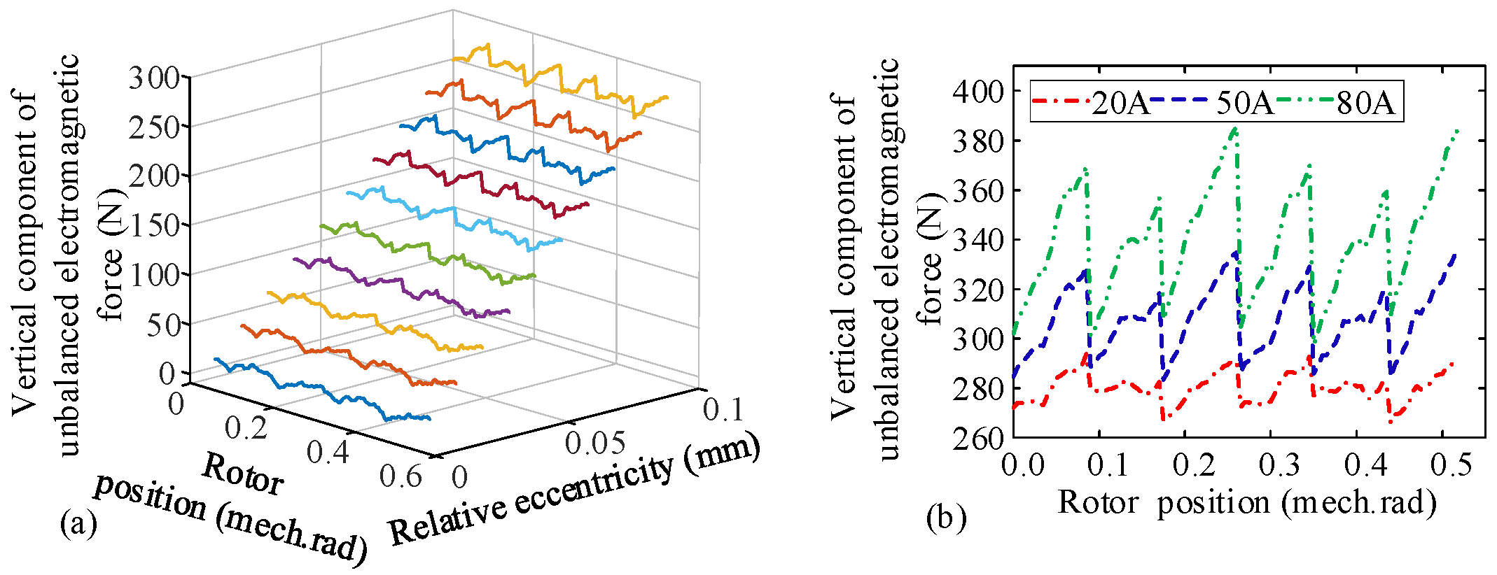
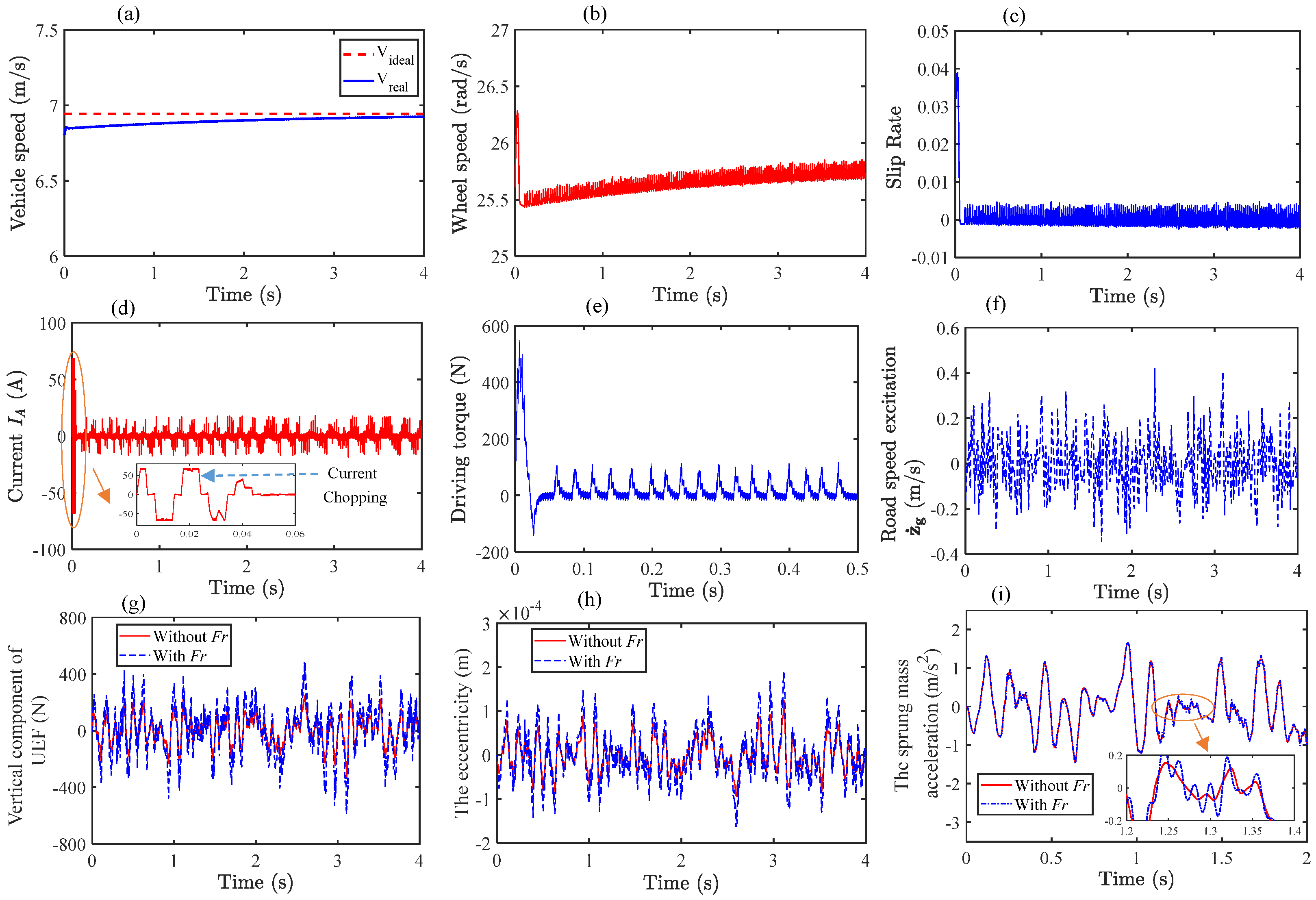
2.2. Characteristics of UEF and Its Influence on the Vehicle Performance

In this paper, the rotor pole-pair number of PMBDC motor adopted is 12. Thus, rotational angular of the rotor is 2π/12 = 0.52 (rad) in one PWM duty cycle, as shown in Figure 2b. For above-mentioned mathematical formulas, it can be found that UMF is a function of rotor position ${{\displaystyle \int }}^{}{\omega }_{r}dt,$ phase currents (I_A, I_B, I_C) and eccentricity e_d (z). Figure 4a shows the influence of the eccentricity and rotor position on UEF when the phase current is 20A. It can be observed that the mean value of UEF rises rapidly with the minor increase of the eccentricity. Similarly, Figure 4b presents the relationship between the rotor eccentricity, phase current and UMF when the rotor eccentricity is 0.1 mm. The mean value and amplitude value of the UEF rise as the phase current increases. By examining the influence of the eccentricity, rotor position and the phase current on the UEF, it can be noted that the sensitivity of the eccentricity is greater than the sensitivity of the rotor position and phase current. This means that the discussion of the eccentricity is of great significance.

The parameters of the hub-driven EV are listed in the Appendix A. Based on the electric vehicle model driven by IWM established in Section 2.1, the performance of an electric vehicle with a passive suspension was investigated at a speed of 25 km/h on a B-class road (Figure 5). Figure 5a shows the error between the ideal and real vehicle speed; Figure 5b–f describe wheel speed (rotor speed), slip rate, A-phase current of IWM, driving torque T_e produced by PMBDC motor, and road speed excitation, respectively. It can be observed that all signals are reasonable, indicating that the model established is correct. Figure 5g–i describe the vertical component of the UEF, the eccentricity of rotor and the acceleration of the body with or without coupling effect, respectively. In Figure 5, the coupling effect is considered if there is F_r, while it is not considered if there is no F_r. It can be concluded that the coupling effect exacerbates the electromagnetic force oscillation, increases the eccentricity of the rotor, and aggravates the acceleration of sprung mass. The eccentricity of rotor provokes UEF, as shown in Figure 4a. Synchronously, the UEF intensifies the eccentricity, as shown in Figure 5e. This mutual promotion phenomenon aggravates the electromagnetic coupling effect, thus intensifying the wear of bearing and shortening the life of the motor. Furthermore, it aggravates the acceleration of sprung mass and provokes cacophony, deteriorating the vehicle comfort. Therefore, the coupling effect in IWM should be seriously considered when designing active suspension system for hub-driven EVs.

2.3. Active Suspension System Modelling

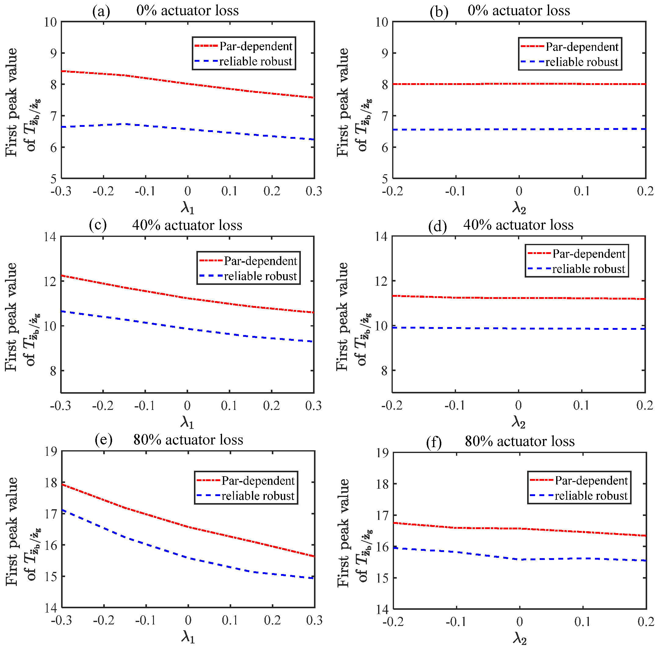
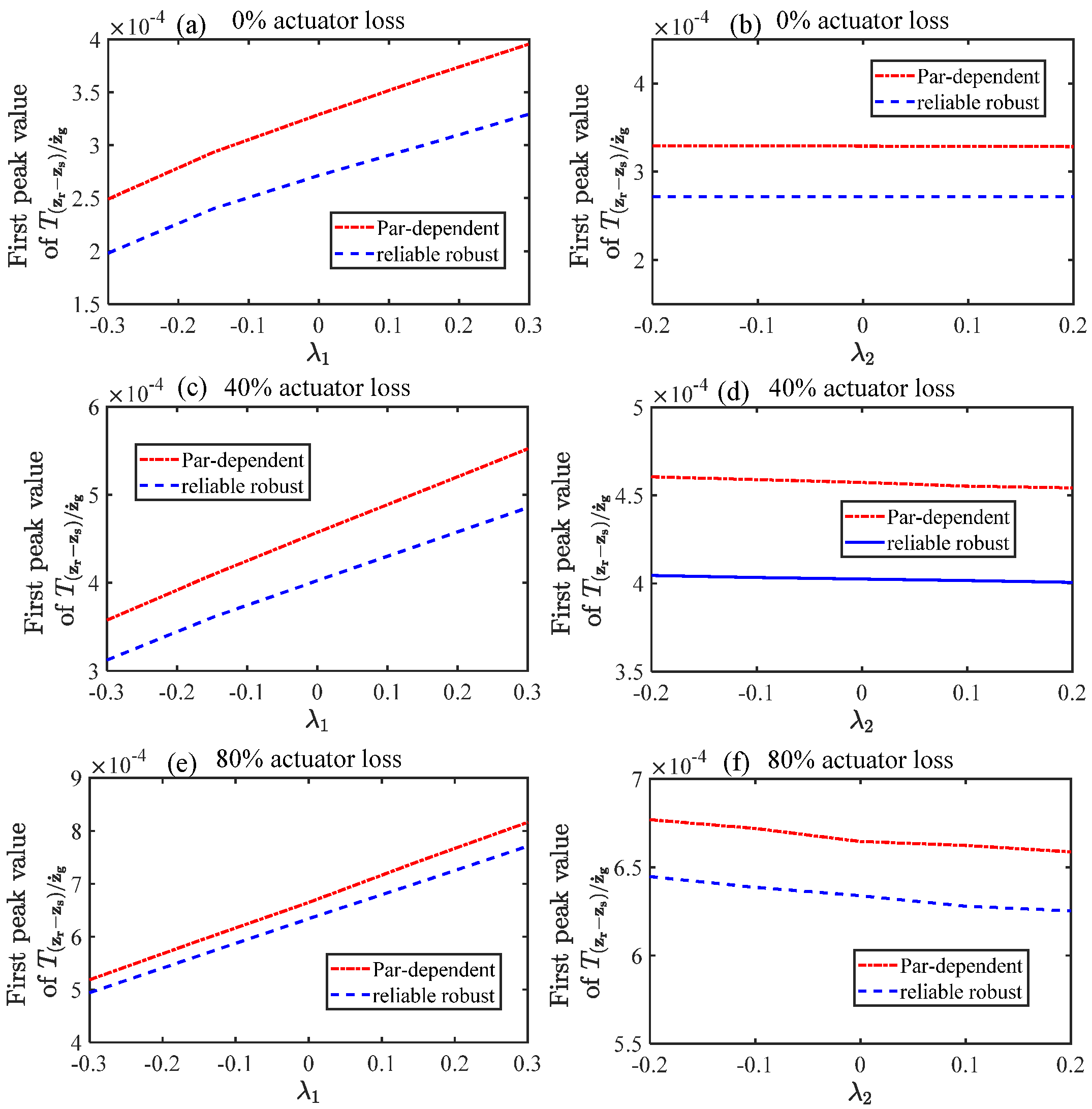
The sprung mass m_b includes the driver mass and passenger mass, so it usually changes with the number of drivers and passengers. The tire stiffness k_t usually varies due to tire pressure. In this study, it is supposed that the sprung mass and the tire stiffness reside in an interval as follows:

$$m_b=m_{b0}(1+{\lambda }_1) k_t=k_{t0}(1+{\lambda }_2)$$

(19)

where m_b0 and k_t0 are the nominal sprung mass and the nominal tire stiffness, respectively. $\left|{\lambda }_1\right|\le {\lambda }_{10}$ and $\left|{\lambda }_2\right|\le {\lambda }_{20}$ are used to exhibit the interval that the sprung mass and the tire stiffness are located within. Furthermore, $m_{bl}=m_{b0}\left(1+{\lambda }_1\right){|}_{\lambda 1=-\lambda 10}$ and $k_{tl}=k_{t0}\left(1+{\lambda }_2\right){|}_{\lambda 2=-\lambda 20}$ are, respectively, expressed as the lower bounds of the sprung mass and the tire stiffness. Similarly, $m_{bu}=m_{b0}\left(1+{\lambda }_1\right){|}_{\lambda 1=\lambda 10}$ and $k_{tu}=k_{t0}\left(1+{\lambda }_2\right){|}_{\lambda 2=\lambda 20}$ are expressed as the corresponding upper bounds. Therefore, the uncertain parameter vector can be described as $\lambda =\left[{\lambda }_1,{\lambda }_2\right]$.

According to Equation (11), and defining vehicle state vector as

$$x(t)={\left[\begin{array}{cccccc}{\dot{z}}_b& {\dot{z}}_s& {\dot{z}}_r& z_s-z_b& z_r-z_s& z_g-z_r\end{array}\right]}^T$$

(20)

the dynamic model of the vehicle can be described by the following state-space equations.

$$\dot{x}(t)=A(\lambda )x(t)+B_1(\lambda )w(t)+B_2(\lambda )\xi u(t)$$

(21)

where

$$\begin{array}{c}A(\lambda )=\left[\begin{array}{cccccc}-c_s{m}_b^{-1}& c_s{m}_b^{-1}& 0& k_s{m}_b^{-1}& 0& 0\\ c_s{m}_s^{-1}& -c_s{m}_s^{-1}& 0& -k_s{m}_s^{-1}& k_m{m}_s^{-1}& 0\\ 0& 0& -c_t{m}_r^{-1}& 0& -k_m{m}_r^{-1}& k_t{m}_r^{-1}\\ -1& 1& 0 & 0& 0& 0\\ 0& -1& 1& 0& 0& 0\\ 0& 0& -1& 0& 0 & 0\end{array}\right], B_1(\lambda )={\left[\begin{array}{cccccc}0& 0& c_t{m}_r^{-1}& 0& 0& 1\\ 0& m_s^{-1}& -m_r^{-1}& 0& 0& 0\end{array}\right]}^T,\hfill \\ B_2(\lambda )={\left[\begin{array}{cccccc}{m}_b^{-1}& -m_s^{-1}& 0& 0& 0& 0\end{array}\right]}^T, w(t)={\left[\begin{array}{cc}{\dot{z}}_g& F_r\end{array}\right]}^T,\hfill \end{array}$$

where λ represents uncertain parameter vector and u(t) is the actuator force produced by active suspension. As shown in Figure 6a, the active suspension system consists of an electro-magnetic actuator and a mechanical spring. Fail safe passive damping is provided by means of eddy-currents. The linear motor actuator is a tubular slotted three-phase permanent magnet actuator with a peak force of 2000 N. The actuator is shown as Figure 6b, where ${\tau }_p$ represents the PM pole pitch; $R_s$ represents the coils outer radius; ${\tau }_{cp}$ and ${\tau }_{sp}$ represent the coil and slot pitches, respectively; ${\tau }_{mz}$ and ${\tau }_{mr}$ denote the pitches of axially and radially magnetized PMs, respectively; ${\tau }_s$ represents the slot width; and $R_0$ and $R_m$ represent the inner and outer radii of the PMs. The details can be found in the literature [51,52]. The thrust force according to axial direction is shown in Figure 6c (detailed calculation of the thrust force can be found in literature [52]).

3. Reliable Robust H_ꝏ Controller Design

Traditionally, most studies mainly consider three requirements, namely, road-holding stability, suspension deflection, and the ride comfort, when designing a control law for suspension systems. Some studies also take energy-saving into consideration. However, few papers have covered the coupling performance of IWMs in suspension design, especially for PMSM. The issues for active suspension system associated with actuator fault tolerance, model parameter uncertainties and coupling effect in IWM based on PMSM have not been well studied in any previous research. Therefore, the reliable robust H∞ control law for active suspension of hub-driven EVs is designed. Considering factors mentioned above, the following suspension performances should be taken into account.

(1). Maximum actuator force. The active control force provided by the suspension system should be constrained by a threshold due to the limited power of the actuator, that is

$$\left|u(t)\right|\le u_{\max }$$

(22)

where u_max is the maximum force of the actuator.

(2). Ride comfort. To provide comfort for passengers, a control u is designed to isolate the sprung mass from the road and magnetic force induced vibration, i.e., to minimize the vertical acceleration ${\ddot{z}}_b$ in the presence of parameter uncertainties m_b and k_t, unknown dynamics F_r, and road speed excitation.

(3). Suspension deflection. The suspension deflection should not exceed its travel limit to avoid ride comfort degradation and vehicle component damage. i.e.,

$$\left|z_s(t)-z_b(t)\right|\le z_{\max }$$

(23)

where z_max is the maximum deflection of the suspension.

(4). Motor unbalance dynamic force. The UEF in IWM promotes the rotor eccentricity which intensifies the bearing wear, shortening the motor life. Furthermore, it aggravates the sprung mass acceleration and provokes cacophony, deteriorating the vehicle comfort significantly. As previously analyzed, the UEF is closely related to the rotor eccentricity. Thus, another primary objective is to minimize the rotor eccentricity when the controller is designed. That is, $\left|z_r-z_s\right|$.

(5). Road-holding stability. The firm uninterrupted contact of wheels to road should be ensured to make sure the vehicle safety, that is to say, the dynamic load of the tire should not exceed its corresponding static load, i.e.,

$$k_t(z_r(t)-z_g(t))\le (m_b+m_s+m_r)g$$

(24)

To analyze the performances mentioned above, for the sake of convenience the controlled outputs are defined as

$$z_1={\left[\begin{array}{cc}{\ddot{z}}_b& \beta (z_r-z_s)\end{array}\right]}^T\hspace{1em}\hspace{1em}{z}_2={\left[\begin{array}{cc}\gamma \frac{z_s(t)-z_b(t)}{z_{\max }}& \frac{k_t(z_r(t)-z_g(t))}{(m_b+m_s+m_r)g}\end{array}\right]}^T$$

(25)

Thus, active suspension control system can be described by a state-space equation as:

$$\{\begin{array}{l}\dot{x}(t)=A(\lambda )x(t)+B_1(\lambda )w(t)+B_2(\lambda )u(t)\\ z_1=C_1(\lambda )x(t)+D_1(\lambda )u(t)\\ z_2=C_2(\lambda )x(t)+D_{2}u(t)\end{array}$$

(26)

where

$$\begin{array}{c}{C}_1(\lambda )=\left[\begin{array}{cccccc}-c_s{m}_b^{-1}& c_s{m}_b^{-1}& 0& k_s{m}_b^{-1}& 0& 0\\ 0& 0& 0& 0& \beta & 0\end{array}\right],D_1(\lambda )={\left[\begin{array}{cc}{m}_b^{-1}& 0\end{array}\right]}^T,\hfill \\ C_2(\lambda )=\left[\begin{array}{cccccc}0& 0& 0& \gamma z^{-1}{}_{\max }& 0& 0\\ 0& 0& 0& 0& 0& k_t{(m_b+m_s+m_r)}^{-1}{g}^{-1}\end{array}\right],D_2={[0 0]}^T,\hfill \end{array}$$

where γ and β are weight coefficients. To obtain a better control performance of the suspension, a state-feedback controller as u_d = k(λ)x(t) is designed. Then, by considering the actuator fault, a state-feedback controller can be modelled as

$$u_{actual}(t)=\xi u_d=\xi k(\lambda )x(t)$$

(27)

where $k\left(\lambda \right)$ is a gain matrix of the feedback controller that needs to be determined, ξ represents the possible actuator fault, u_d is the desired force calculated by the controller, and u_actual is the actual force generated by the actuator. Assuming that ξ is constrained by its maximum ξ_max value and minimum value ξ_min, the control law considering actuator faults and parameter uncertainties can be denoted as

$$u_{actual}(t)=\xi k(\lambda )x(t)={\xi }_0(I+L)k(\lambda )x(t)$$

(28)

where ${\xi }_0=\left({\xi }_{max}+{\xi }_{min}\right)/2$ and $L=\left(\xi -{\xi }_0\right)/{\xi }_0$. Defining $\mathrm{J}=\left({\xi }_{max}-{\xi }_{min}\right)/\left({\xi }_{max}+{\xi }_{min}\right)$, then, we have $L^{T}L\le {\mathrm{J}}^T\mathrm{J}\le \mathrm{I}$.

Therefore, the closed-loop system with state-feedback controller is rewritten as:

$$\begin{array}{l}\dot{x}(t)=(A(\lambda )+{\xi }_0(I+L)B_2(\lambda )k(\lambda ))x(t)+B_1(\lambda )w(t)\\ z_1=C_1(\lambda )x(t)+D_1(\lambda )u(t) z_2=C_2(\lambda )x(t)+D_{2}u(t)\end{array}$$

(29)

where the system matrices A(λ), B₁(λ), B₂(λ), C₁(λ), D₂(λ) and C₂(λ), which are dependent on the sprung mass m_b and the tire stiffness k_t, are functions of λ. It is assumed that A(λ), B₁(λ), B₂(λ), C₁(λ), D₂(λ) and C₂(λ) are constrained within the polytope Ω

$$\Omega =\left\{\begin{array}{c}(A,{{\rm B}}_1,B_2,C_1,D_1,C_2)(\lambda ):\\ (A,B_1,B_2,C_1,D_1,C_2)(\lambda )={\displaystyle \sum _{i=1}^4{a}_i(\lambda )(A,B_1,B_2,C_1,D_1,C_2)(i),}\\ {\displaystyle \sum _{i=1}^4{a}_i(\lambda )=1, a_i(\lambda )\ge 1,}\end{array}\right\}$$

(30)

where

$$\begin{array}{l}{(A,B_1,B_2,C_1,D_1,C_2)}_1=(A(\lambda ),B_1(\lambda ),B_2(\lambda ),C_1(\lambda ),D_1(\lambda ),C_2(\lambda )){|}_{{\lambda }_1=-{\lambda }_{10},{\lambda }_2=-{\lambda }_{20}}\\ {(A,B_1,B_2,C_1,D_1,C_2)}_2=(A(\lambda ),B_1(\lambda ),B_2(\lambda ),C_1(\lambda ),D_1(\lambda ),C_2(\lambda )){|}_{{\lambda }_1=-{\lambda }_{10},{\lambda }_2={\lambda }_{20}}\\ {(A,B_1,B_2,C_1,D_1,C_2)}_3=(A(\lambda ),B_1(\lambda ),B_2(\lambda ),C_1(\lambda ),D_1(\lambda ),C_2(\lambda )){|}_{{\lambda }_1={\lambda }_{10},{\lambda }_2=-{\lambda }_{20}}\\ {(A,B_1,B_2,C_1,D_1,C_2)}_4=(A(\lambda ),B_1(\lambda ),B_2(\lambda ),C_1(\lambda ),D_1(\lambda ),C_2(\lambda )){|}_{{\lambda }_1={\lambda }_{10},{\lambda }_2={\lambda }_{20}}\end{array}$$

Additionally, the relationship between the uncertain masses (m_b and k_t) and the vector $a\left(\lambda \right)=\left(a_1\left(\lambda \right),a_2\left(\lambda \right),a_3\left(\lambda \right),a_4\left(\lambda \right)\right)$ is expressed by

$$\begin{array}{l}{a}_1(\lambda )=M_1(\lambda )\times N_1(\lambda ) a_2(\lambda )=M_1(\lambda )\times N_2(\lambda )\\ a_3(\lambda )=M_2(\lambda )\times N_1(\lambda ) a_4(\lambda )=M_2(\lambda )\times N_2(\lambda )\end{array}$$

(31)

where

$$\begin{array}{l}{M}_1(\lambda )=\left(m_b^{-1}-m_{bu}^{-1}\right)/\left(m_{bl}^{-1}-m_{bu}^{-1}\right) M_2(\lambda )=\left(m_{bl}^{-1}-m_b^{-1}\right)/\left(m_{bl}^{-1}-m_{bu}^{-1}\right)\\ N_1(\lambda )=\left(k_t^{-1}-k_{tu}^{-1}\right)/\left(k_{tl}^{-1}-k_{tu}^{-1}\right) N_2(\lambda )=\left(k_{rl}^{-1}-k_r^{-1}\right)/\left(k_{rl}^{-1}-k_{ru}^{-1}\right)\end{array}$$

Lemma 1.

[18] For matices R and S, the inequality $\mathrm{R}\mathsf{\Sigma }\mathrm{S}+{\mathrm{S}}^T{\mathsf{\Sigma }}^T{\mathrm{R}}^T\le \epsilon {\mathrm{RVR}}^T+{\epsilon }^{-1}{\mathrm{S}}^T\mathrm{VS}$ holds, if ε > 0, $\mathsf{\Sigma }\left(t\right)=diag\left(\sigma {\left(t\right)}_1,\sigma {\left(t\right)}_2,\dots ,\sigma {\left(t\right)}_p\right)$ is a time varying diagonal matrix, and satisfies $\left|\mathsf{\Sigma }\right|\le \mathrm{V}$.

Theorem 1.

For given positive constant ρ, a robust reliable H_∞ controller in the form of Equation (28) exists, such that the closed-loop system in Equation (29) is asymptotically stable and satisfies$\Vert {\mathrm{z}}_1{\left(t\right)\Vert }_2<\gamma \Vert \mathrm{w}{\left(t\right)\Vert }_2$for all w satisfying$\Vert \mathrm{w}{\left(t\right)\Vert }_2^2\le \Vert \mathrm{w}{\left(t\right)\Vert }_{max}=\rho /{\gamma }^2$, while the constrains in inequalities (32–34) are guaranteed, if there exist symmetric matrices$\overline{\mathrm{P}}\left(\mathsf{\lambda }\right)$, general matrix$\overline{\mathrm{k}}\left(\mathsf{\lambda }\right)$and any scalar$\eta >0$, $\epsilon >0$satisfying

$$\left[\begin{array}{ccccc}{\overline{\Lambda }}_{11}& B_1(\lambda )& {\overline{\Lambda }}_{13}& \eta B_2& {\overline{k}}^T(\lambda ){\xi }_0^T\\ \ast & -{\gamma }^{2}I& 0& 0& 0\\ \ast & \ast & -I& \eta D_1(\lambda )& 0\\ \ast & \ast & \ast & -\eta J^{-1}& 0\\ \ast & \ast & \ast & \ast & -\eta J^{-1}\end{array}\right]<0$$

(32)

$$\left[\begin{array}{ccc}-I+\epsilon J& \sqrt{\rho }{\xi }_0\overline{k}(\lambda )& 0\\ \ast & -u_{\max }^2\overline{P}(\lambda )& \sqrt{\rho }{\overline{k}}^T(\lambda ){\xi }_0^T\\ \ast & \ast & \epsilon J^{-1}\end{array}\right]<0$$

(33)

$$\left[\begin{array}{cc}-I& \sqrt{\rho }{C}_2(\lambda )\overline{P}(\lambda )\\ \ast & -z_{\max }^2\overline{P}(\lambda )\end{array}\right]<0$$

(34)

with

$${\overline{\Lambda }}_{11}=\mathrm{sym}(A(\lambda )\overline{P}(\lambda )+B_2(\lambda ){\xi }_0\overline{k}(\lambda )), {\overline{\Lambda }}_{13}=\overline{P}(\lambda )C_1^T(\lambda )+{\overline{k}}^T(\lambda ){\xi }_0^T{D}_1^T(\lambda ).$$

Proof. 

Choose the Lyapunov–Krasovskii functional candidate as follows:

$$\mathrm{v}(t,\lambda )=x^T(t)P(\lambda )x(t)$$

(35)

To establish a system in Equation (29) that is robust asymptotically stable with disturbance attenuation $\gamma >0$, the following Hamiltonian should be less than zero

$$\mathrm{H}(x,\lambda ,w,t)=z_1^T(t)z_1(t)-{\gamma }^2{w}^T(t)w(t)+\dot{v}(\lambda ,t)<0$$

(36)

$$\begin{array}{cc}\hfill \mathrm{H}(x,\lambda ,w,t)=& x^T(t)\{{[A(\lambda )+B_2(\lambda ){\xi }_0(I+L)k(\lambda )]}^{T}P(\lambda )+P(\lambda )[A(\lambda )+B_2(\lambda ){\xi }_0(I+L)k(\lambda )]\}x(t)+\hfill \\ & x^T(t)P(\lambda )B_1(\lambda )w(t)+ w{(t)}^T{B_1}^T(\lambda )P(\lambda )x(t)-{\gamma }^{2}w{(t)}^{T}w(t)+x^T(t) [C_1(\lambda )+\hfill \\ & D_1(\lambda ){\xi }_0(I+L)k(\lambda ){]}^T[C_1(\lambda )+D_1(\lambda ){\xi }_0(I+L)k(\lambda )]x(t)\hfill \\ \hfill =& {\Gamma }^T(t)\left[\begin{array}{cc}{\Pi }_1& P(\lambda )B_1(\lambda )\\ B_1{}^T(\lambda )P(\lambda )& -{\gamma }^{2}I\end{array}\right]{\Gamma }^T(t)\hfill \end{array}$$

where

$$\begin{gathered} {\Gamma }^T(t)=[x^T(t),w{(t)}^T{]}^T \\ \begin{array}{l}{\Pi }_1={[A(\lambda )+B_2(\lambda ){\xi }_0(I+L)k(\lambda )]}^{T}P(\lambda )+P(\lambda )[A(\lambda )+B_2(\lambda ){\xi }_0(I+L)k(\lambda )]+\\ {[C_1(\lambda )x(t)+ D_1(\lambda ){\xi }_0(I+L)k(\lambda )]}^T[C_1(\lambda )x(t)+D_1(\lambda ){\xi }_0(I+L)k(\lambda )] \end{array} \end{gathered}$$

To achieve $\mathrm{H}\left(\mathrm{x},\mathsf{\lambda },\mathrm{w},t\right)<0$ for all $\mathsf{\Gamma }\left(t\right)\ne 0$, the following inequality should hold

$$\left[\begin{array}{cc}{\Pi }_1& P(\lambda )B_1(\lambda )\\ B_1{}^T(\lambda )P(\lambda )& -{\gamma }^{2}I\end{array}\right]<0$$

(37)

By using the Schur complement, inequality (37) can be converted into inequality (38).

$$\begin{array}{l}\left[\begin{array}{ccc}{\Lambda }_{11}& P(\lambda )B_1(\lambda )& {\Lambda }_{13}\\ \ast & -{\gamma }^{2}I& 0\\ \ast & \ast & -I\end{array}\right]+\left[\begin{array}{c}P(\lambda )B_2(\lambda )\\ 0\\ D_1(\lambda )\end{array}\right]L\left[\begin{array}{ccc}{\xi }_{0}k(\lambda )& 0& 0\end{array}\right]\\ +{\left(\left[\begin{array}{c}P(\lambda )B_2(\lambda )\\ 0\\ D_1(\lambda )\end{array}\right]L\left[\begin{array}{ccc}{\xi }_{0}k(\lambda )& 0& 0\end{array}\right]\right)}^T<0\end{array}$$

(38)

where

$${\Lambda }_{11}=\mathrm{sym}(P(\lambda )A(\lambda )+P(\lambda )B_2(\lambda ){\xi }_{0}k(\lambda )), {\Lambda }_{13}={[C_1(\lambda )+D_1(\lambda ){\xi }_{0}k(\lambda )]}^T.$$

Based on Lemma 1, inequality (38) can be converted into inequality (39).

$$\left[\begin{array}{ccc}{\Psi }_{11}& P(\lambda )B_1(\lambda )& {\Psi }_{13}\\ \ast & -{\gamma }^{2}I& 0\\ \ast & \ast & -I+\eta D_1(\lambda )J{D}_1^T(\lambda )\end{array}\right]<0$$

(39)

where

$${\Psi }_{11}={\Lambda }_{11}+\eta P(\lambda )B_2(\lambda )B_2^T(\lambda )P(\lambda )+k^T(\lambda ){\xi }_0^T{\eta }^{-1}J{\xi }_{0}k(\lambda ), {\Psi }_{13}={\Lambda }_{13}+\eta P(\lambda )B_{2}J{D}_1^T(\lambda ).$$

By the Schur complement, we get

$$\left[\begin{array}{ccccc}{\Lambda }_{11}& P(\lambda )B_1(\lambda )& {\Lambda }_{13}& \eta P(\lambda )B_2& k^T(\lambda ){\xi }_0^T\\ \ast & -{\gamma }^{2}I& 0& 0& 0\\ \ast & \ast & -I& \eta D_1(\lambda )& 0\\ \ast & \ast & \ast & -\eta J^{-1}& 0\\ \ast & \ast & \ast & \ast & -\eta J^{-1}\end{array}\right]<0$$

(40)

Pre- and post-multiplying diag $\left\{\mathrm{P}{\left(\lambda \right)}^{-1} \mathrm{I} \mathrm{I} \mathrm{I} \mathrm{I}\right\}$, the congruent transformation of the matrix is achieved. Subsequently, by defining $\overline{P}\left(\lambda \right)=\mathrm{P}{\left(\lambda \right)}^{-1}$ and $\overline{k}\left(\lambda \right)=k\left(\lambda \right)\mathrm{P}{\left(\lambda \right)}^{-1}$, the inequality (40) is equivalent to the first LMI in inequality (32). Then we will show that hand constrains in inequalities (22)–(24) are guaranteed. From the Lyapunov function in inequality (35), it can be known that $x^T\mathrm{Px}<\rho$, with $\rho ={\gamma }^2{\mathbf{w}}_{\mathit{max}}+\mathrm{v}\left(0\right)$. Similarly, the following inequalities hold:

$$\begin{array}{cc}\underset{t>0}{\max }{\left|u(t)\right|}^2& =\underset{t>0}{\max }{\Vert {\xi }_0(I+L)k(\lambda )x(t)\Vert }_2^2=\underset{t>0}{\max }{\Vert x{(t)}^T{[{\xi }_0(I+L)k(\lambda )]}^T[{\xi }_0(I+L)k(\lambda )]x(t)\Vert }_2\hfill \\ & <\rho \cdot {\theta }_{\max }(P^{-1/2}{[{\xi }_0(I+L)k(\lambda )]}^T[{\xi }_0(I+L)k(\lambda )]P^{-1/2})<u_{\max }^{2}I\hfill \end{array}$$

(41)

$$\begin{array}{l}\underset{t>0}{\max }{\left|\left\{z_2(t)\right\}\right|}^2=\underset{t>0}{\max }{\Vert x{(t)}^T{C}_2{(\lambda )}^T{C}_2(\lambda )x(t)\Vert }_2\\ =\underset{t>0}{\max }{\Vert \left\{x{(t)}^{T}P{(\lambda )}^{1/2}P{(\lambda )}^{-1/2}{C}_2{(\lambda )}^T{C}_2(\lambda )P{(\lambda )}^{-1/2}P{(\lambda )}^{1/2}x(t)\right\}\Vert }_2\\ \hspace{0.17em} <\rho \cdot {\theta }_{\max }(P{(\lambda )}^{-1/2}{C}_2{(\lambda )}^T{C}_2(\lambda )P{(\lambda )}^{-1/2})<z_{\max }^{2}I\end{array}$$

(42)

where ${\theta }_{max}(\cdot )$ represents the maximal eigenvalue. Using the Schur complement and Lemma 1, inequality (41) can be written as

$$\left[\begin{array}{ccc}-I+\epsilon J& \sqrt{\rho }{\xi }_{0}k(\lambda )& 0\\ \ast & -u_{\max }^{2}P(\lambda )& \sqrt{\rho }{k}^T(\lambda ){\xi }_0^T\\ \ast & \ast & \epsilon J^{-1}\end{array}\right]<0$$

(43)

Pre- and post-multiplying inequality (43) by diag $\left\{\mathrm{I} \mathrm{P}{\left(\lambda \right)}^{-1} \mathrm{I} \right\}$, defining $\overline{P}\left(\lambda \right)=\mathrm{P}{\left(\lambda \right)}^{-1}$ and $\overline{k}\left(\lambda \right)=k\left(\lambda \right)\mathrm{P}{\left(\lambda \right)}^{-1}$, the inequality is equivalent to the second LMI in inequality (33). Furthermore, based on the Schur complement, the inequality matrix in inequality (42) can be change to

$$\left[\begin{array}{cc}-I& \sqrt{\rho }{C}_2(\lambda )\\ \ast & -z_{\max }^{2}P(\lambda )\end{array}\right]<0$$

(44)

Pre- and post-multiplying inequality (44) by diag $\left\{\mathrm{I} \mathrm{P}{\left(\lambda \right)}^{-1}\right\}$, using $\overline{P}\left(\lambda \right)$ to replace $\mathrm{P}{\left(\lambda \right)}^{-1}$, the LMI inequality (44) is equal to the third LMI in inequality (34). Thus, the proof is completed.

According to the inner property of the polytopic tire stiffness uncertainties and sprung mass uncertainties, Equations (32)–(34) in Theorem 1 are equivalent to the inequalities as follows:

$$\left[\begin{array}{ccccc}{\overline{\overline{\Lambda }}}_{11}& B_{1i}& {\overline{\overline{\Lambda }}}_{13}& {\eta }_{ij}{B}_{2i}& {\overline{k}}_j^T{\xi }_0^T\\ \ast & -{\gamma }^{2}I& 0& 0& 0\\ \ast & \ast & -I& {\eta }_{ij}{D}_{1i}& 0\\ \ast & \ast & \ast & -{\eta }_{ij}{J}^{-1}& 0\\ \ast & \ast & \ast & \ast & -{\eta }_{ij}{J}^{-1}\end{array}\right]<0\hspace{0.17em}\hspace{0.17em}i,j=1,2,3,4$$

(45)

$$\left[\begin{array}{ccc}-I+{\epsilon }_{j}J& \sqrt{\rho }{\xi }_0\overline{k}{}_j& 0\\ \ast & -u_{\max }^2{\overline{P}}_j& \sqrt{\rho }{\overline{k}}_j^T{\xi }_0^T\\ \ast & \ast & {\epsilon }_j{J}^{-1}\end{array}\right]<0\hspace{0.17em}\hspace{0.17em}j=1,2,3,4$$

(46)

$$\left[\begin{array}{cc}-I& \sqrt{\rho }{C}_{2i}{\overline{P}}_j\\ \ast & -z_{\max }^2{\overline{P}}_j\end{array}\right]<0\hspace{0.17em}\hspace{0.17em}i,j=1,2,3,4$$

(47)

where

$${\overline{\overline{\Lambda }}}_{11}=\mathrm{sym}(A_i{\overline{P}}_j+B_{2i}{\xi }_0{\overline{k}}_j), {\overline{\overline{\Lambda }}}_{13}={\overline{P}}_j{C}_{1i}^T+{\overline{k}}_j^T{\xi }_0^T{D}_{1i}^T.$$

Thus, by solving the following convex optimization problem, the robust state-feedback controller design can be accomplished.

min γ

s.t. inequalities (45)–(47), ${\overline{P}}_j>0$, ${\eta }_{ij}>0$, ${\epsilon }_j>0$

for ${\overline{k}}_j$, i, j = 1, 2, 3, 4,

The gain matrix of the controller can be expressed by

$$K=\xi \left({\displaystyle \sum _{j=1}^4{a}_j(\lambda ){\overline{k}}_j}\right){\left({\displaystyle \sum _{j=1}^4{a}_j(\lambda ){\overline{P}}_j}\right)}^{-1}$$

(48)

This convex optimization problem can be solved by the function mincx provided by MATLAB. Employing a similar method to what is proposed in Theorem 1, the theorem 2 can be achieved for the active suspension of the hub-driven EVs without actuator faults and parameter uncertainties.

Theorem 2.

Given positive constant ρ, a H_∞ controller exists, such that the closed-loop system is asymptotically stable and satisfies $\Vert z_1{\left(t\right)}_2\Vert <\gamma \Vert \mathrm{w}{\left(t\right)\Vert }_2$ for all w satisfying $\Vert \mathrm{w}{\left(t\right)\Vert }_2^2\le \Vert \mathrm{w}{\left(t\right)\Vert }_{max}=\rho /{\gamma }^2$, while the constrains in inequalities (22–24) are guaranteed, if there exist symmetric matrices P and general matrix k satisfying

$$\left[\begin{array}{ccc}\mathrm{sym}(AP+B_{2}k)& B_1& P{C}_1^T+k^T{D}_1^T\\ \ast & -{\gamma }^{2}I& 0\\ \ast & \ast & -I\end{array}\right]<0$$

(49)

$$\left[\begin{array}{cc}-I& \sqrt{\rho }k\\ \ast & -u_{\max }^{2}p\end{array}\right]<0$$

(50)

$$\left[\begin{array}{cc}-I& \sqrt{\rho }{C}_{2}P\\ \ast & -z_{\max }^{2}P\end{array}\right]<0$$

(51)

Thus, the feedback gain matrix K₂ of the controller can be given by $K_2={\mathrm{k}P}^{-1}$.

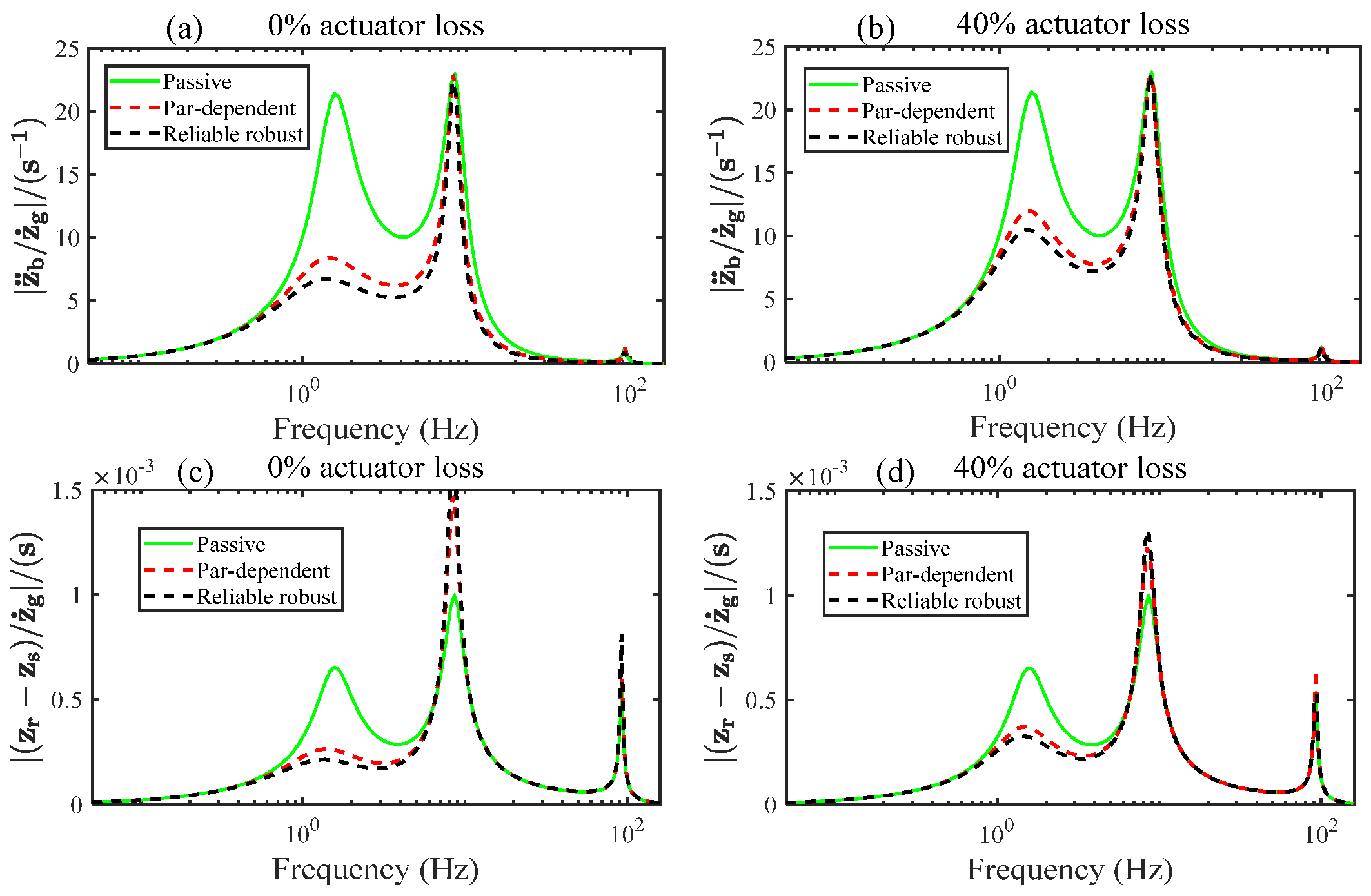
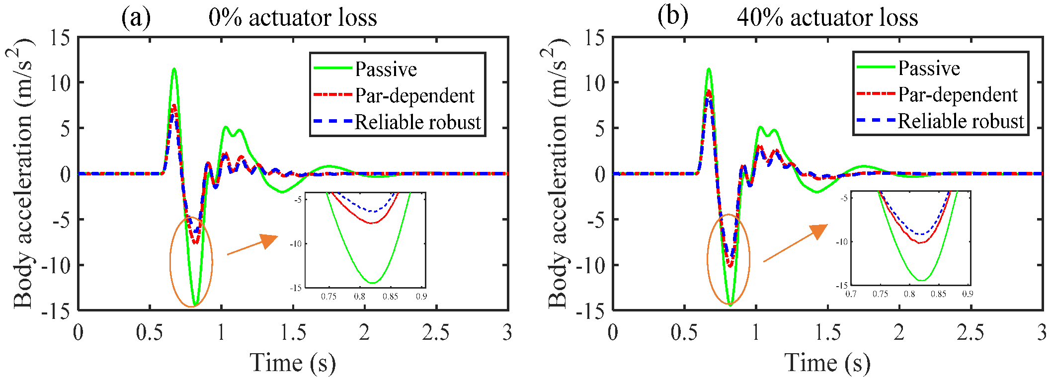
4. Results and Discussion

To reflect the superiority of reliable robust H_∞ controller in improving the vehicle and the motor performances, the responses of the hub-driven EV under different controllers are investigated in both the frequency domain and time domain. The parameters of the hub-driven EV are given in Appendix A. We assume $u_{max}=2000 \mathrm{N}$ and $z_{max}=0.11 \mathrm{m}$. Moreover, the uncertain parameters about the sprung mass and the tire stiffness are supposed to satisfy $\left|{\lambda }_1\right|\le 0.3$, $\left|{\lambda }_2\right|\le 0.2$.

A conventional robust controller K_C is designed firstly, as described by Theorem 2, in which the actuator failure and the model uncertainties are not considered. The gain matrix of the conventional controller is

$${\mathrm{K}}_{\mathrm{C}}={10}^3\times [-1.092 -0.326 -0.12 -5.802 -4.683 3.91]$$

Then, a parameter-dependent controller K_P is designed for parameter uncertainties by applying the method in Theorem 1 with the ξ₀ and J terms dropped out. This design does not consider the actuator failure, and its corresponding gain matrix is

$${\mathrm{K}}_{\mathrm{P}}={10}^3\times [-0.865 -0.425 -0.109 -6.747 -3.663 4.018]$$

Lastly, a reliable robust controller K_PF is designed for active suspension in the hub-driven EV according to Theorem 1. in which the actuator failure and the parameter uncertainties are both considered. The gain matrix of a reliable robust controller is K_PF1 and K_PF2 when the actuator thrust loss is 0% and 40% respectively.

$$\begin{gathered} {\mathrm{K}}_{\mathrm{PF}1}={10}^3\times [-1.082 -0.531 -0.136 -8.434 -4.579 5.022] \\ {\mathrm{K}}_{\mathrm{PF}2}={10}^3\times [-0.649 -0.319 -0.082 -5.061 -2.747 3.014] \end{gathered}$$

Figure 7 illustrates the control structure for the active suspension system. The control structure can be divided into two parts: the outer control loop and the inner control loop. In the inner control loop, the states which are sampled by sensors act as an input to the reliable robust Hꝏ controller. The ideal control force is first generated by the controller based on control strategy. Then, the linear motor is controlled to produce thrust force (detailed control process can be found in the literature [52]). In the outer control loop, with the change of the sprung mass, tire stiffness or actuator thrust losses exceed a certain limit, the gain matrix of the controller will be updated by solving proposed convex optimization problem. This convex optimization process takes 20 s. However, the degree of actuator thrust loss, the sprung mass, and the tire stiffness do not change rapidly in real time. In other words, the gain matrix of the controller is not updated in real time. In addition, in inner control loop, the absolute CPU-time (0.00081 s) per time step is shorter than the real-time simulation time-step (0.01 s), thus illustrating the viability of its real-time implementation.

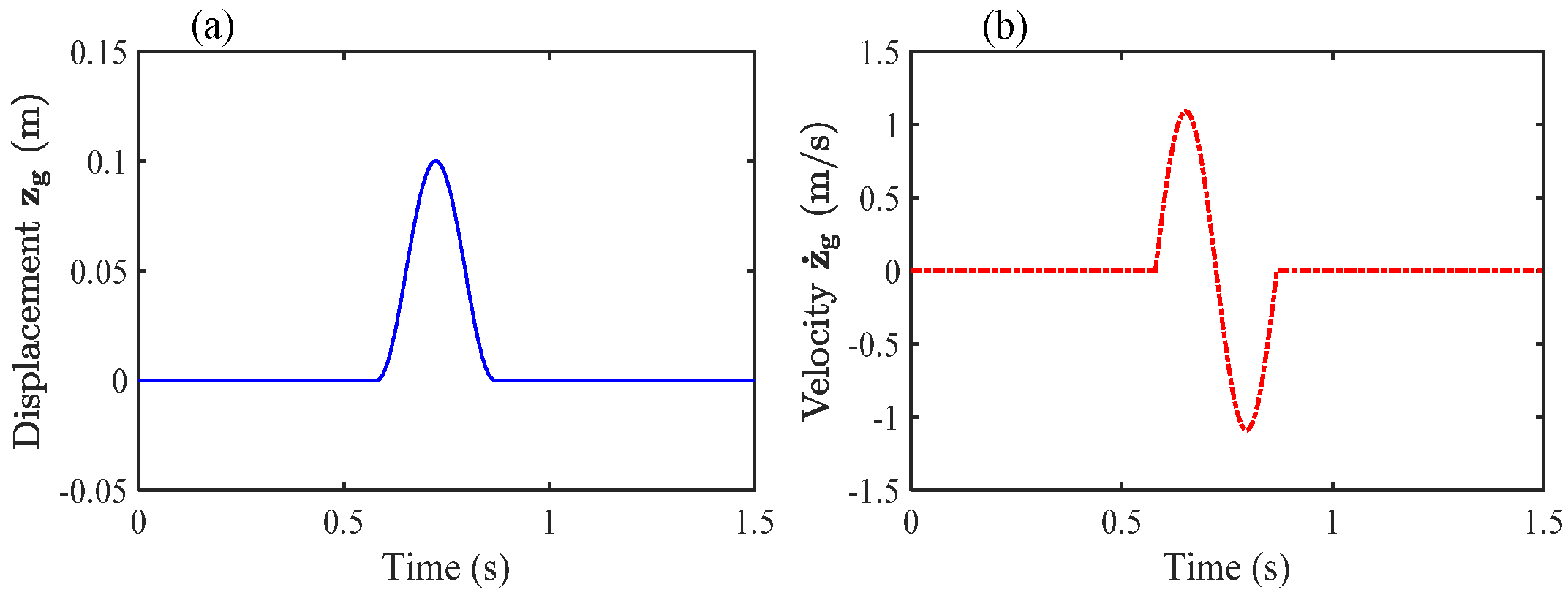
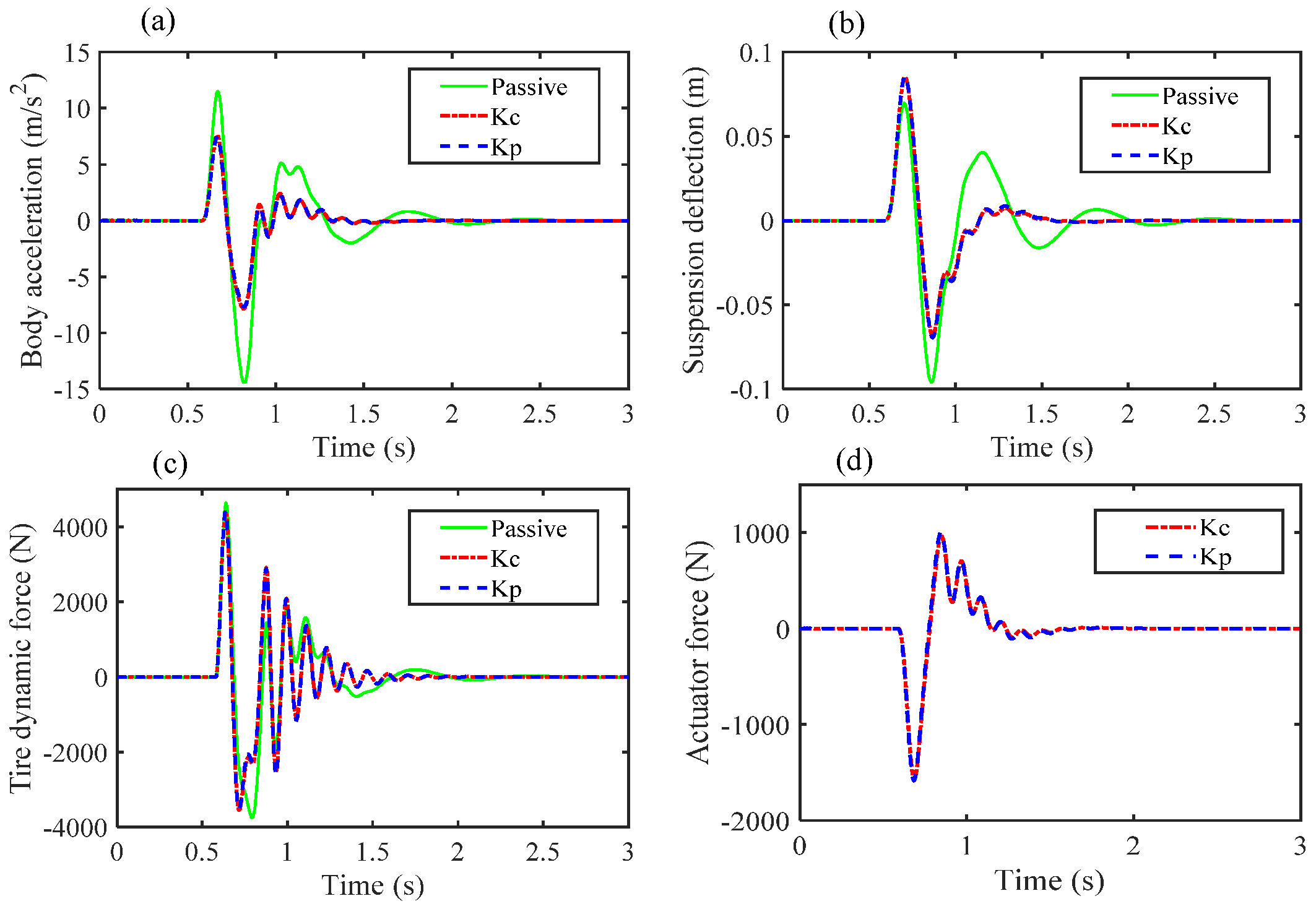
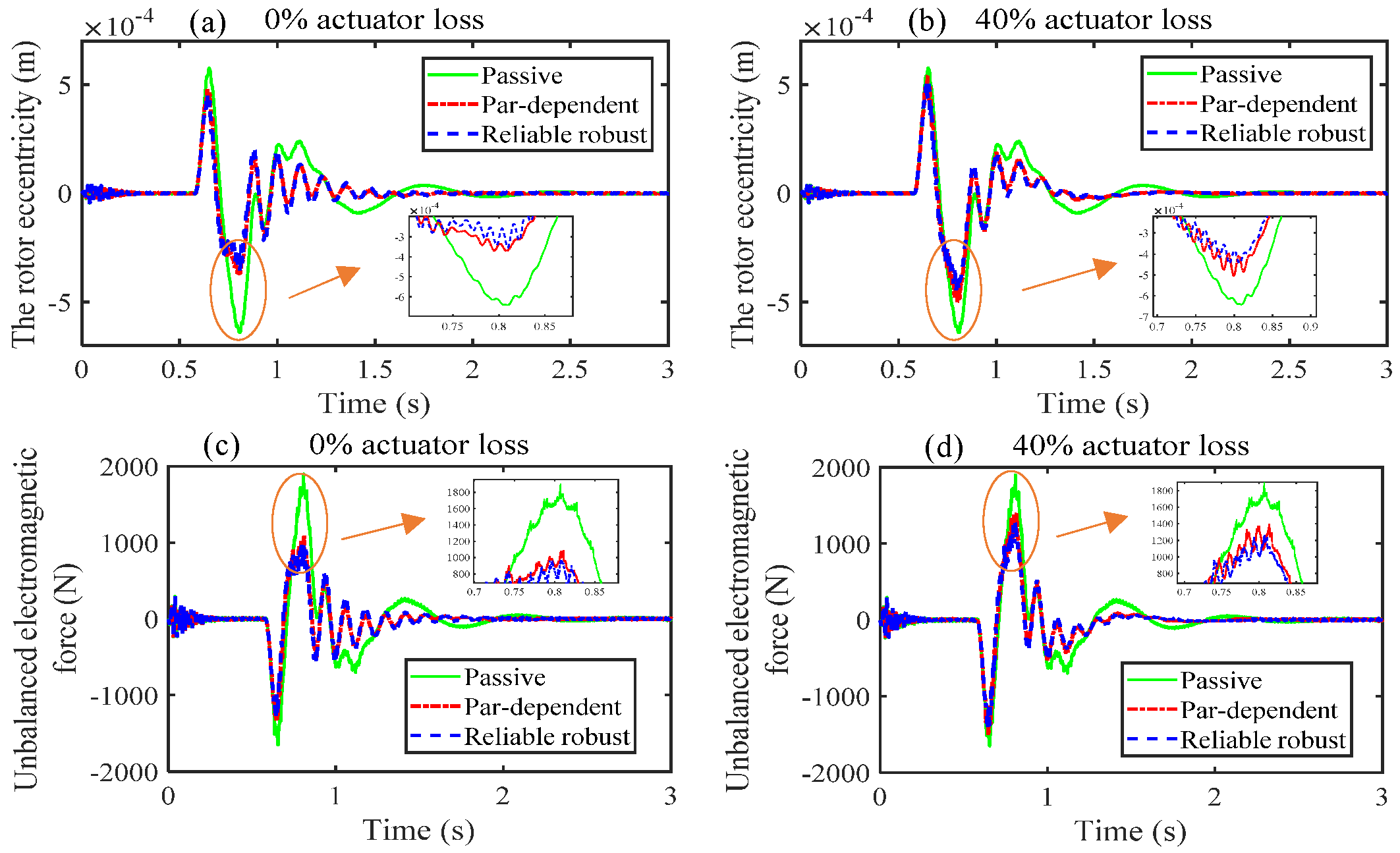
4.1. Bump Road Excitation

To reveal the transient response characteristics of the electric vehicle and the IWM, the bumpy road excitation is introduced as follows:

$$z_g=\{\begin{array}{cc}\frac{a}{2}(1-\cos (\frac{2\pi v_0}{l}t)),& t_0\le t\le \frac{l}{v_0}+t_0\hfill \\ 0,& t>l/v_0+t_0\hfill \end{array}$$

(52)

where a denotes the height of the bump; l denotes the length of the bump; v₀ denotes vehicle forward velocity. Here we choose v₀ = 25 km/h, l = 0.2 m and a = 0.1 m. Figure 8a,b show the road displacement excitation and speed excitation, respectively.

Figure 9 shows the time-domain responses of passive suspension, K_C and K_P. It can be observed that, compared with passive suspension, the body acceleration, tire dynamic force and suspension deflection of active suspension with K_C and K_P are obviously reduced. Furthermore, the periods of their transients become much shorter. These imply that the performance of the electric vehicle has been improved with active control system. In addition, it can be observed that the control effects of K_C and K_P are similar in time domain.

Besides, the corresponding responses of the rotor eccentricity and the UEF of IWM are illustrated in Figure 10. It can be seen that the magnitudes of the eccentricity and the UEF under active suspension are significantly reduced in time domain, indicating that the active suspension greatly improve the performance of the IWM. The reason behind this is that active suspension inhibits the rotor eccentricity, restricting the magnetic force oscillation. Thus, the coupling effect in IWM is alleviated.

Figure 11a,b show the frequency responses from the ground velocity to the body vertical acceleration for the open and closed-loop systems using the conventional robust controller and the parameter-dependent controller. It can be observed that the closed-loop system minimizes the acceleration of the sprung mass in the frequency range from 1 Hz to 8 Hz implying that the ride comfort of EV is enhanced. The parameter-dependent controller for active suspension systems achieve less value of sprung mass acceleration than the conventional robust controller. It means that the control effect of the parameter-dependent controller is slightly better. In addition, the second peak value of $T_{{\ddot{z}}_b/{\dot{z}}_g}$, which decreases with an increase in the sprung mass, is the fixed point for active suspension system.

Figure 11c,d demonstrate the frequency responses from the ground velocity to the rotor eccentricity for the open and closed-loop systems. It can be seen that the closed-loop system reduces the value of $T_{\left(z_r-z_g\right)/{\dot{z}}_g}$ in the frequency range from 1 Hz to 4 Hz, implying that active suspension can suppress the interference from the ground to the IWM in the corresponding frequency range, alleviating the coupling effect in IWM.

Figure 11e,f show the frequency responses from the F_r (UEF) to the body vertical acceleration for the open and closed-loop systems. One can observe that the closed-loop system can suppress the influence of the UEF on the body vertical acceleration, improving the ride comfort of EV. Compared with the conventional robust controller, the parameter-dependent controller performs better in frequency domain.

Figure 12 shows the first peak value of the closed-loop transfer function $T_{{\ddot{z}}_b/{\dot{z}}_g}$ with the parameter-dependent controller and the reliable robust controller versus the uncertain parameters λ₁ and λ₂ in existence of 0%, 40%, and 80% actuator thrust loss. One can observe that the peak value of $T_{{\ddot{z}}_b/{\dot{z}}_g}$ goes up with an increase of actuator thrust loss. This indicates that, with the extent of failure increasing, the effect of active suspension to isolate the disturbance from the ground to the sprung mass becomes worse, deteriorating the ride comfort. In addition, one can observe that, along with the changes of the uncertain parameters λ₁ and λ₂, the reliable robust controller yields smaller closed-loop peak value than the parameter-dependent controller, indicating that the reliable robust controller considering actuator fault-tolerant can achieve better the ride comfort of EV than the one without fault-tolerant.

Figure 13 shows the first peak value of the closed-loop transfer function $T_{\left(z_r-z_g\right)/{\dot{z}}_g}$ with the parameter-dependent controller and the reliable robust controller versus the uncertain parameters λ₁ and λ₂ in the existence of 0%, 40%, and 80% actuator thrust loss. Clearly, under different actuator thrust loss, the reliable robust controller can obtain outstanding performances in terms of isolating the disturbance from the ground to the IWM, compared with the parameter-dependent controller. In addition, one can observed that the peak value of $T_{\left(z_r-z_g\right)/{\dot{z}}_g}$ goes up with an increase of λ₁, indicating that with the increase of sprung mass, the effect of active suspension to isolate the disturbance from the ground to the IWM becomes worse. That is to say, the increase of the sprung mass intensifies coupling effect in IWM.

Figure 14 shows the frequency responses of the open and closed-loop systems by using the parameter-dependent controller and the reliable robust controller in the existence of 0% and 40% actuator thrust loss. Similar to Figure 11a,b, one can observe that compared with passive suspension and the parameter-dependent controller, the reliable robust controller can achieve better vehicle and motor performance, when actuator thrust loss occurs.

Figure 15 and Figure 16 illustrate the time-domain responses of passive suspension and active suspension with the parameter-dependent controller and the reliable robust controller in the existence of 0% and 40% actuator thrust loss. Similar to Figure 13, those figures reveal the advantage of the reliable robust controller in improving the ride comfort and inhibiting the coupling effect in IWM.

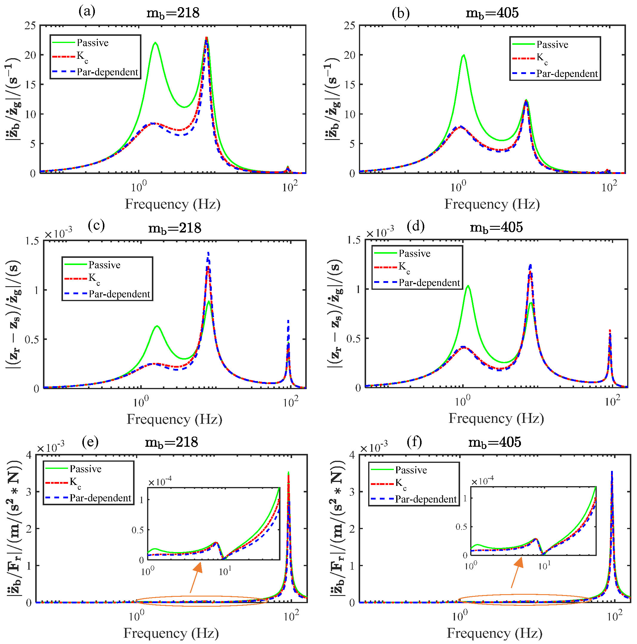
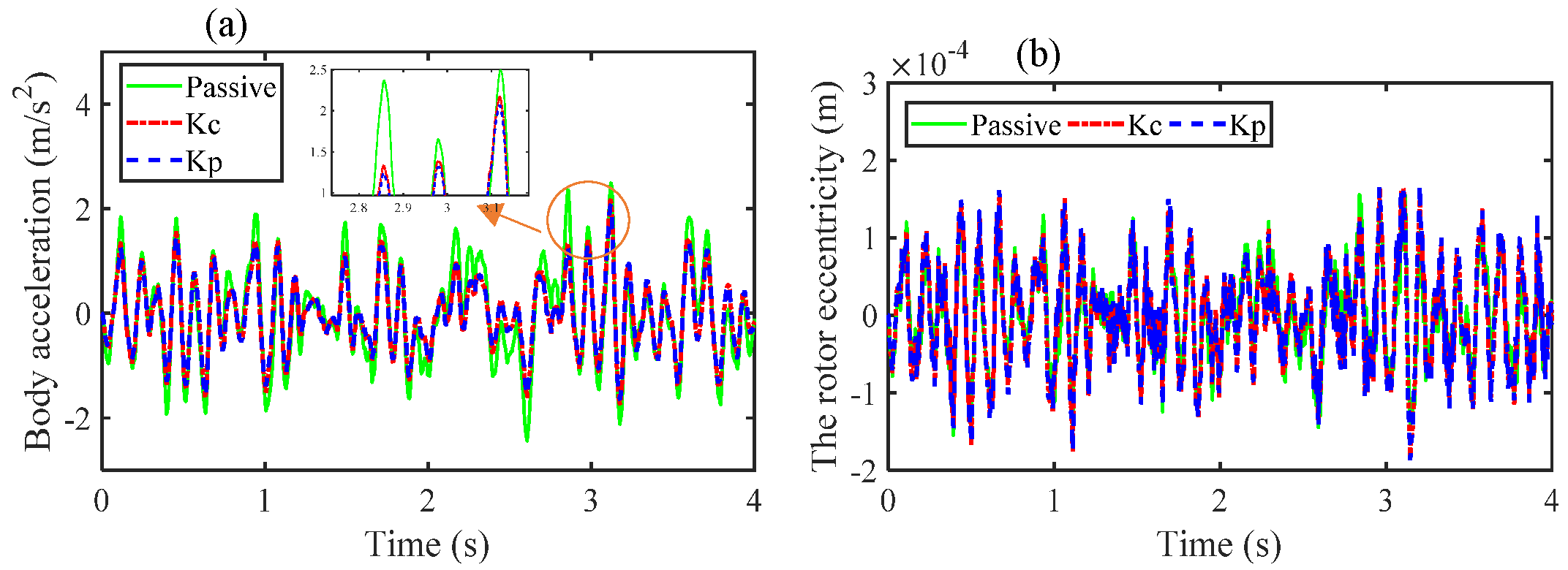
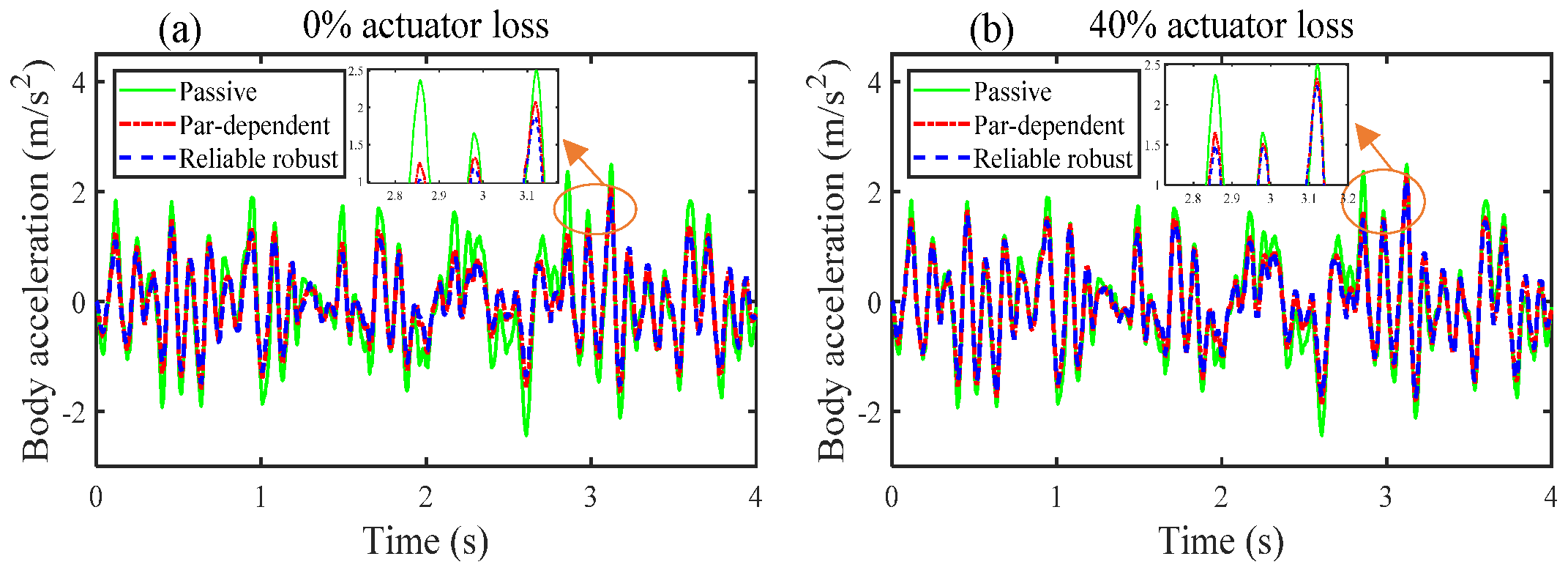
4.2. Random Road Excitation

To further evaluate the advantages of the reliable robust controller, the performances of electric vehicles are investigated at a speed of 25 km/h on a B-class road. Figure 17 and

Table 1. The root mean square (RMS) of electric vehicle (EV) responses.

Dynamics Response	Passive	Active Suspension
		Kc	KP
Sprung mass acceleration (m/s2)	0.92	0.70	0.67
Deflection of suspension (m)	0.0046	0.0043	0.0045
Dynamic force of tire (N)	647.7	787	819
Eccentricity (m)	6.1 × 10−5	6.4 × 10−5	6.5 × 10−5
UEF (N)	164.4	174.5	176
Control force (N)	--	90.97	103.3

show the stochastic responses of three suspensions (K_C, K_P, and the passive suspension). Responses of the sprung mass acceleration and the rotor eccentricity are plotted in Figure 17. A detailed numerical comparison using the root mean square values (RMS) is shown in Table 1. One can observe that both of active control methods K_C and K_P can obviously enhance the ride comfort and slightly intensify the rotor eccentricity compared with passive suspension. It can be found that compared with K_C, the RMS of the sprung mass acceleration controlled by K_P decreased by 4.5%, from 0.7 to 0.67, and the rotor eccentricity only rose by 0.8%, from 174.5 to 176. The comprehensive performance of K_P is obvious better than that of K_C.

Figure 18 and

Table 2. The RMS of EV dynamic responses with different actuator thrust losses and parameter variation.

Suspension Types	Body Accele-Ration (m/s2)	Suspension Deflection (m)	Tire Dynamic Force (N)	Control Force (N)	Eccentricity (m)	UEF (N)
Passive	0.92	0.0046	647.7	--	6.1 × 10−5	164.4
Pra-dependent 0%	0.67	0.0045	819	103.3	6.5 × 10−5	176
Reliable robust 0%	0.61	0.0047	893.9	136.5	6.9 × 10−5	187.5
Pra-dependent 40%	0.77	0.0043	732.4	58.9	6.1 × 10−5	166.1
Reliable robust 40%	0.72	0.0043	761.4	74.6	6.1 × 10−5	169.2
Pra-dependent 80%	0.86	0.0044	671.1	19.5	5.9 × 10−5	160.9
Reliable robust 80%	0.85	0.0044	677.7	24.3	5.9 × 10−5	161.0

show the stochastic responses of three suspensions (K_P, K_PF and the passive suspension). It can be seen from Table 2 and Figure 18 that the reliable robust controller achieves a lower peak value and lower RMS value of sprung mass acceleration, compared with passive system and the parameter-dependent controller system without actuator fault-tolerant, which clearly illustrates that K_PF can effectively improve the ride comfort. Furthermore, from Table 2, it can be observed that when the extent of failure is minor, the RMS of the body acceleration is greatly reduced and the RMS of the UEF increased slightly compared to passive suspension and the parameter-dependent control system. The results imply that the reliable robust controller with slight actuator failure can significantly enhance the ride comfort and avoid large increases of the coupling effect in IWM. When the extent of failure is major, both the body acceleration and the UEF decreased to a certain extent, indicating that the ride comfort and the IWM performance are improved. According to the analysis, it can be inferred that in the presence of actuator failure and model parameter uncertainties, the active suspension system with the reliable robust controller improves the ride comfort and PMBDC motor operation performance.

In general, the active suspension system considering the eccentricity of the rotor can greatly enhance the ride comfort and weaken the influence of UEF on the performance of the hub-driven EV. When the model parameters are perturbed, the parameter-dependent controller shows better comprehensive performance than conventional robust controller_. In addition, the reliable robust controller can achieve better vehicle and motor performance in the presence of different actuator thrust losses and parameter variation, compared with the conventional robust controller and parameter-dependent controller.

5. Conclusions

The mathematical model for a hub-driven electric vehicle considering the coupling effect in IWM was established based on electric magnetic field theory. The influences of the coupling effect on the vehicle performances were analyzed. Then, a reliable robust Hꝏ controller considering model uncertainties, actuator failure and electromagnetic force interference was designed. The results are given as follows:

(1). The vertical UEF in the motor is strongly coupled with rotor rotation position, phase current, and rotor eccentricity. High phase current and large rotor eccentricity promoted by the coupling effect provoke the UEF of the motor. The mutual promotion phenomenon (i.e., the rotor eccentricity provokes the UEF; synchronously, the UEF intensifies the rotor eccentricity) aggravates the electromagnetic coupling effect, thus worsening the motor operation performance. Furthermore, this phenomenon aggravates the car body acceleration, deteriorating the ride comfort of vehicle.

(2). Based on Lyapunov stability theory, a reliable robust Hꝏ controller for active suspension of a hub-driven EV associated with model uncertainties, actuator failure, and electromagnetic force interference was investigated. The control objective is to enhance the ride comfort and restrict the coupling effect in IWM while satisfying the hard constraints such as road holding capability, suspension deflection limitation, actuator failure, and parameter variation. Simulation results in both the frequency-domain and time-domain show the robustness and advantageous performances of the reliable robust Hꝏ controller method. This work can provide a practical model reference for the study of vibration performance of hub-driven EVs with PMSM and the optimization, control and improvement of its vibration performance. In the future, the influence of bearing nonlinear force and bearing clearance on the ride comfort and the motor operation performance will be studied. Moreover, the experimental validation will be investigated.

References

1. Wang, Z.; Qu, C.; Zhang, L.; Xue, X.; Wu, J. Optimal component sizing of a four-wheel independently-actuated electric vehicle with a real-time torque distribution strategy. IEEE Access 2018, 6, 49523–49536. [Google Scholar] [CrossRef]
2. Long, G.; Ding, F.; Zhang, N.; Zhang, J.; Qin, A. Regenerative active suspension system with residual energy for in-wheel motor driven electric vehicle. Appl. Energy 2020, 260, 114180. [Google Scholar] [CrossRef]
3. Mingchun, L.; Feihong, G.; Yuanzhi, Z. Ride Comfort Optimization of In-Wheel-Motor Electric Vehicles with In-Wheel Vibration Absorbers. Energies 2017, 10, 1647–1668. [Google Scholar]
4. Teixeira, A.C.; Sodré, J.R. Impacts of replacement of engine powered vehicles by electric vehicles on energy consumption and CO 2 emissions. Transp. Res. Part D-Transp. Environ. 2018, 59, 375–384. [Google Scholar] [CrossRef]
5. Zhao, W.; Wang, Y.; Wang, C. Multidisciplinary optimization of electric-wheel vehicle integrated chassis system based on steady endurance performance. J. Clean Prod. 2018, 186, 640–651. [Google Scholar] [CrossRef]
6. Xu, B.; Xiang, C.; Qin, Y.; Ding, P.; Dong, M. Semi-active vibration control for in-wheel switched reluctance motor driven electric vehicle with dynamic vibration absorbing structures: Concept and validation. IEEE Access 2018, 6, 60274–60285. [Google Scholar] [CrossRef]
7. Song, C.X.; Xiao, F.; Song, S.X.; Peng, S.L.; Fan, S.Q. Stability Control of 4WD Electric Vehicle with In-Wheel Motors Based on Integrated Control of Electro-Mechanical Braking System. Appl. Mech. Mater. 2015, 740, 206–210. [Google Scholar] [CrossRef]
8. Zhai, L.; Sun, T.; Wang, J. Electronic Stability Control Based on Motor Driving and Braking Torque Distribution for a Four In-Wheel Motor Drive Electric Vehicle. IEEE Trans. Veh. Technol. 2016, 65, 4726–4739. [Google Scholar] [CrossRef]
9. Sun, W.; Li, Y.; Huang, J.; Zhang, N. Vibration effect and control of In-Wheel Switched Reluctance Motor for electric vehicle. J. Sound Vibr. 2015, 338, 105–120. [Google Scholar] [CrossRef]
10. Qin, Y.; He, C.; Shao, X.; Du, H.; Xiang, C.; Dong, M. Vibration mitigation for in-wheel switched reluctance motor driven electric vehicle with dynamic vibration absorbing structures. J. Sound Vibr. 2018, 419, 249–267. [Google Scholar] [CrossRef]
11. Tan, D.; Wang, H.; Wang, Q. Study on the Rollover Characteristic of In-Wheel-Motor-Driven Electric Vehicles Considering Road and Electromagnetic Excitation. Shock Vib. 2016, 2016, 13. [Google Scholar] [CrossRef]
12. Luo, Y.; Tan, D. Study on the dynamics of the In-Wheel Motor System. IEEE Trans. Veh. Technol. 2012, 61, 3510–3518. [Google Scholar]
13. Zhao, Y.E.; Zhang, J.W.; Han, X. Design and study on the dynamic damper mechanism for an in-wheel motor individual drive electric vehicle. Mech. Sci. Technol. Aerosp. Eng. 2008, 27, 395–398. [Google Scholar]
14. Li, Z.; Zheng, L.; Ren, Y.; Li, Y.; Xiong, Z. Multi-objective optimization of active suspension system in electric vehicle with In-Wheel-Motor against the negative electromechanical coupling effects. Mech. Syst. Signal Proc. 2019, 116, 545–565. [Google Scholar] [CrossRef]
15. Shao, X.; Naghdy, F.; Du, H.; Qin, Y. Coupling effect between road excitation and an in-wheel switched reluctance motor on vehicle ride comfort and active suspension control. J. Sound Vibr. 2019, 443, 683–702. [Google Scholar] [CrossRef]
16. Wang, R.; Jing, H.; Yan, F.; Karimi, H.R.; Chen, N. Optimization and finite-frequency H∞ control of active suspensions in in-wheel motor driven electric ground vehicles. J. Frankl. Inst. 2015, 352, 468–484. [Google Scholar] [CrossRef]
17. Qin, Y.; He, C.; Ding, P.; Dong, M.; Huang, Y. Suspension hybrid control for in-wheel motor driven electric vehicle with dynamic vibration absorbing structures. IFAC-PapersOnLine 2018, 51, 973–978. [Google Scholar] [CrossRef]
18. Shao, X.; Naghdy, F.; Du, H.; Li, H. Output feedback H∞ control for active suspension of in-wheel motor driven electric vehicle with control faults and input delay. ISA Trans. 2019, 92, 94–108. [Google Scholar] [CrossRef]
19. Jing, H.; Wang, R.; Li, C.; Wang, J.; Chen, N. Fault-tolerant control of active suspensions in in-wheel motor driven electric vehicles. Int. J. Veh. Des. 2015, 68, 22–36. [Google Scholar] [CrossRef]
20. R, J.; Choi, S.B. A novel semi-active control strategy based on the quantitative feedback theory for a vehicle suspension system with magneto-rheological damper saturation. Mechatronics 2018, 54, 36–51. [Google Scholar]
21. Liu, B.; Saif, M.; Fan, H. Adaptive fault tolerant control of a half-car active suspension systems subject to random actuator failures. IEEE-Asme Trans. Mechatron. 2016, 21, 2847–2857. [Google Scholar] [CrossRef]
22. Yetendje, A.; Seron, M.; De Dona, J. Diagnosis and Actuator Fault Tolerant Control in Vehicle Active Suspension. In Proceedings of the 2007 Third International Conference on Information and Automation for Sustainability, Melbourne, VIC, Australia, 4–6 December 2007; pp. 153–158. [Google Scholar]
23. Cao, F.; Sun, H.; Li, Y.; Tong, S. Fuzzy Adaptive Fault-Tolerant Control for a Class of Active Suspension Systems with Time Delay. Int. J. Fuzzy Syst. 2019, 21, 2054–2065. [Google Scholar] [CrossRef]
24. Jing, H.; Wang, R.; Karimi, H.R.; Chadli, M.; Hu, C.; Yan, F. Robust output-feedback based fault-tolerant control of active suspension with finite-frequency constraint. IFAC-Pap. 2015, 48, 1173–1179. [Google Scholar] [CrossRef]
25. Liu, S.; Zhou, H.; Luo, X.; Xiao, J. Adaptive sliding fault tolerant control for nonlinear uncertain active suspension systems. J. Frankl. Inst. 2016, 353, 180–199. [Google Scholar] [CrossRef]
26. Ma, M.; Chen, H.; Liu, X. Robust H-infinity control for constrained uncertain systems and its application to active suspension. J. Control Theory Appl. 2012, 10, 470–476. [Google Scholar] [CrossRef]
27. Sun, W.; Pan, H.; Yu, J.; Gao, H. Reliability control for uncertain half-car active suspension systems with possible actuator faults. IET Contr. Theory Appl. 2014, 8, 746–754. [Google Scholar] [CrossRef]
28. Haiping, D.; Zhang, N. Fuzzy control for nonlinear uncertain electrohydraulic active suspensions with input constraint. IEEE Trans. Fuzzy Syst. 2008, 17, 343–356. [Google Scholar] [CrossRef]
29. Zhang, Y.; Zhang, G.; Yu, F. Modeling and μ Synthesis Control of Vehicle Active Suspension with Motor Actuator. WSEAS Trans. Syst. 2012, 11, 173–186. [Google Scholar]
30. Pang, H.; Liu, F.; Xu, Z. Variable universe fuzzy control for vehicle semi-active suspension system with MR damper combining fuzzy neural network and particle swarm optimization. Neurocomputing 2018, 3, 130–140. [Google Scholar] [CrossRef]
31. Akay, H.; Türkay, S. Influence of tire damping on mixed H2/H∞ synthesis of half-car active suspensions. J. Sound Vib. 2009, 322, 15–28. [Google Scholar] [CrossRef]
32. Pusadkar, U.S.; Chaudhari, S.D.; Shendge, P.D.; Phadke, S.B. Linear disturbance observer based sliding mode control for active suspension systems with non-ideal actuator. J. Sound Vib. 2019, 442, 428–444. [Google Scholar] [CrossRef]
33. Chen, S.L.; Chen, S.H.; Yan, S.T. Stabilization of a Current-Controlled Three-Pole Magnetic Rotor-Bearing System by Integral Aliding Mode Control. In Proceedings of the IEEE International Conference on Networking, Sensing and Control, Taipei, Taiwan, 21–23 March 2004. [Google Scholar]
34. Wu, H.; Wu, J.; Sun, Q.; Wang, H.; Zhang, L. A Novel Sliding Mode Observer-Based Sensorless PMSM Control. In Proceedings of the 2019 22nd International Conference on Electrical Machines and Systems (ICEMS), Harbin, China, 11–14 August 2019; pp. 1–5. [Google Scholar]
35. Mystkowski, A. Lyapunov sliding-mode observers with application for active magnetic bearing operated with zero-bias flux. J. Dyn. Syst. Meas. Control 2019, 141, 041006. [Google Scholar] [CrossRef]
36. Hezzi, A.; Bensalem, Y.; Elghali, S.B.; Abdelkrim, M.N. Sliding Mode Observer Based Sensorless Control of Five Phase PMSM in Electric Vehicle. In Proceedings of the 2019 19th International Conference on Sciences and Techniques of Automatic Control and Computer Engineering (STA), Sousse, Tunisia, 24–26 March 2019. [Google Scholar]
37. Pang, H.; Zhang, X.; Xu, Z. Adaptive backstepping-based tracking control design for nonlinear active suspension system with parameter uncertainties and safety constraints. ISA Trans. 2019, 88, 23–36. [Google Scholar] [CrossRef] [PubMed]
38. Sun, L.; Wang, X. Nonlinear Control for Semi-active Suspension with Input Constraints. IFAC-Pap. 2018, 51, 131–135. [Google Scholar] [CrossRef]
39. Mystkowski, A.; Pawluszewicz, E. Nonlinear Position-Flux Zero-Bias Control for AMB System with Disturbance. Appl. Comput. Electromagn. Soc. J. 2017, 32, 650–656. [Google Scholar]
40. Salameh, M.; Yaman, S.; Jiang, Y.; Krishnamurthy, M. Analytical Approach for Calculating Magnetic Field Distribution in Surface Mount PM Motor Including Stator Slot Effect. In Proceedings of the 2019 IEEE Transportation Electrification Conference and Expo (ITEC), Dearborn, MI, USA, 19–21 June 2019; pp. 1–6. [Google Scholar]
41. Ying, M. Configuration Analysis and Structural Research of In-Wheel Motor. Ph.D. Thesis, Chongqing University, Chongqing, China, 2014. [Google Scholar]
42. Zhu, Z.Q.; Howe, D. Instantaneous Magnetic Field Distribution in Brushless Permanent Magnet dc Motors Part 11, Armature-Reaction Field. IEEE Trans. Magn. 1993, 29, 124–135. [Google Scholar] [CrossRef]
43. Zhu, Z.Q.; Ishak, D.; Howe, D.; Chen, J. Unbalanced Magnetic Forces in Permanent-Magnet Brushless Machines with Diametrically Asymmetric Phase Windings. IEEE Trans. Ind. Appl. 2007, 43, 1544–1553. [Google Scholar] [CrossRef]
44. Zhu, Z.Q.; Xia, Z.P.; Wu, L.J.; Jewell, G.W. Analytical Modeling and Finite-Element Computation of Radial Vibration Force in Fractional-Slot Permanent-Magnet Brushless Machines. IEEE Trans. Ind. Appl. 2010, 46, 1908–1918. [Google Scholar] [CrossRef]
45. Zarko, D.; Ban, D.; Lipo, T.A. Analytical calculation of magnetic field distribution in the slotted air gap of a surface permanent-magnet motor using complex relative air-gap permeance. IEEE Trans. Magn. 2006, 42, 1828–1837. [Google Scholar] [CrossRef]
46. Jie, M.; Tao, R.; Lee, X. Analytical calculation of no-load magnetic field distribution in the slotted airgap of a permanent magnet synchronous motor. IFAC Proc. Vol. 2013, 46, 184–189. [Google Scholar] [CrossRef]
47. Kim, D.; Noh, M.D.; Park, Y.W. Unbalanced magnetic forces due to rotor eccentricity in a toroidally wound BLDC motor. IEEE Trans. Magn. 2016, 52, 1–4. [Google Scholar] [CrossRef]
48. Teymoori, S.; Rahideh, A.; Moayed-Jahromi, H.; Mardaneh, M. 2-D analytical magnetic field prediction for consequent-pole permanent magnet synchronous machines. IEEE Trans. Magn. 2016, 52, 1–14. [Google Scholar] [CrossRef]
49. Lu, H.; Zhang, L.; Qu, W. A New Torque Control Method for Torque Ripple Minimization of BLDC Motors with Un-Ideal Back EMF. IEEE Trans. Power Electron. 2008, 23, 950–958. [Google Scholar] [CrossRef]
50. Cabrera, J.A.; Castillo, J.J.; Pérez, J.; Velasco, J.M.; Guerra, A.J.; Hernández, P. A procedure for determining tire-road friction characteristics using a modification of the magic formula based on experimental results. Sensors 2018, 18, 896. [Google Scholar] [CrossRef] [Green Version]
51. Chao, Y. Optimal Design and Energy-Regenerative Research of Electromagnetic Active Suspension Linear Actuator. Ph.D. Thesis, Chongqing University, Chongqing, China, 2018. [Google Scholar]
52. Li, Y.; Zheng, L.; Liang, Y.; Yu, Y. Adaptive compensation control of an electromagnetic active suspension system based on nonlinear characteristics of the linear motor. J. Vib. Control 2020, 42, 386. [Google Scholar] [CrossRef]
Figure 1. Hub-driven electric vehicle model.
Applsci 10 03929 g001
Figure 2. (a) Magnet gap deformation of the in-wheel motor (IWM) (air-gap exaggerated) and (b) the winding distribution of the permanent magnet brushless direct contact (PMBDC) motor.
Applsci 10 03929 g002
Figure 3. IWM-driven system without a speed reducer. (a) Main structure. (b) Quarter vehicle model.
Applsci 10 03929 g003
Figure 4. The characteristics of unbalanced electromagnetic force (UEF): (a) under different rotor position and eccentricity; (b) under different rotor position and phase current.
Applsci 10 03929 g004
Figure 5. The response of the electric vehicle on stochastic uneven road: (a) vehicle speed; (b) wheel speed; (c) slip rate; (d) A-phase current; (e) driving torque; (f) road speed excitation; (g) vertical component of the UEF; (h) the rotor eccentricity; (i) the sprung mass acceleration.
Applsci 10 03929 g005
Figure 6. (a) Electromagnetic suspension system; (b) linear motor actuator structure; (c) thrust force according to axial direction.
Applsci 10 03929 g006
Figure 7. Control structure of the active suspension system.
Applsci 10 03929 g007
Figure 8. Bump input from the ground: (a) displacement excitation; (b) speed excitation.
Applsci 10 03929 g008
Figure 9. Vehicle dynamic responses under bump excitation: (a) body acceleration; (b) suspension deflection; (c) tire dynamic force; (d) actuator force.
Applsci 10 03929 g009
Figure 10. The motor responses under bump excitation: (a) the rotor eccentricity; (b) the UEF.
Applsci 10 03929 g010
Figure 11. Frequency responses for different sprung masses: (a) transfer function T z ¨ b / z ˙ g with m b   = 218; (b) transfer function T z ¨ b / z ˙ g with m b = 405; (c) transfer function T ( z r z g ) / z ˙ g with m b =218; (d) transfer function T ( z r z g ) / z ˙ g with m b = 405; (e) transfer function T z ¨ b / F r with m b = 218; (f) transfer function T z ¨ b / F r with m b = 405.
Applsci 10 03929 g011
Figure 12. The first peak value of T z ¨ b / z ˙ g with the parameter-dependent controller and the reliable robust controller versus the uncertain parameters λ1 and λ2: (a) versus λ1 under 0% actuator loss; (b) versus λ2 under 0% actuator loss; (c) versus λ1 under 40% actuator loss; (d) versus λ2 under 40% actuator loss; (e) versus λ1 under 80% actuator loss; (f) versus λ2 under 80% actuator loss.
Applsci 10 03929 g012
Figure 13. The first peak value of T ( z r z g ) / z ˙ g with the parameter-dependent controller and the reliable robust controller versus the uncertain parameters λ1 and λ2: (a) versus λ1 under 0% actuator loss; (b) versus λ2 under 0% actuator loss; (c) versus λ1 under 40% actuator loss; (d) versus λ2 under 40% actuator loss; (e) versus λ1 under 80% actuator loss; (f) versus λ2 under 80% actuator loss.
Applsci 10 03929 g013
Figure 14. Frequency responses for the open (passive mode) and closed loop (active mode) systems with actuator thrust loss: (a) transfer function T z ¨ b / z ˙ g under 0% actuator loss; (b) transfer function T z ¨ b / z ˙ g under 40% actuator loss; (c) transfer function T ( z r z g ) / z ˙ g under 0% actuator loss; (d) transfer function T ( z r z g ) / z ˙ g under 40% actuator loss.
Applsci 10 03929 g014
Figure 15. Body acceleration of the vehicle: (a) under 0% actuator loss; (b) under 40% actuator loss.
Applsci 10 03929 g015
Figure 16. The in-wheel motor dynamic responses: (a) the rotor eccentricity under 0% actuator loss; (b) the rotor eccentricity under 0% actuator loss; (c) UEF under 0% actuator loss; (d) UEF under 40% actuator loss.
Applsci 10 03929 g016
Figure 17. The responses under stochastic excitation: (a) body acceleration; (b) the rotor eccentricity.
Applsci 10 03929 g017
Figure 18. Body acceleration in electric vehicle: (a) under 0% actuator loss; (b) under 40% actuator loss.
Applsci 10 03929 g018