1. Introduction
Affective Computing is the study and development of systems that have the ability to recognize and process human affective states [
1]. While sensor-based recognition of human physical activity has reached a certain level of maturity, e.g., most mobile devices are nowadays capable of counting steps based on acceleration sensors, the human mental state recognition, e.g., stress, mental health, and cognitive load, remains challenging. Yet, the demand for advancing Affective Computing research is rising, since through improved understanding of its human users, Affective Computing promises to push the frontiers of human–computer interaction (HCI) and to enable new much-needed services that are directly related to psychological states, e.g., mobile healthcare [
2]. One of the main impediment factors for the advance of Affective Computing research is its reliance on real-world user studies that often need to involve elaborate experimental protocols and physiological signal measurements. Being difficult to gather, datasets that include various aspects of human internal states (e.g., the participants’ impressions, personality traits, etc.) as well as detailed physiological signal measurements during the experiments are rare and seldom publicly available.
An important aspect of Affective Computing is the cognitive load inference. There are different reasons why ubiquitous computing devices would benefit from being aware of their users’ cognitive load, the most important of which is likely to prevent the undesirable effects of attention grabbing at times when a user is occupied with a difficult task. Research has repeatedly shown that improperly timed notifications can be distracting, causing a negative effect on task performance [
3,
4,
5,
6,
7,
8], increasing stress [
9], and reducing well-being [
10]. Fortunately, increased cognitive load is reflected in a measurable signal change. When humans experience a psycho-physiological load, e.g., in the form of a demanding task, activation of the sympathetic nervous system increases [
11]. This increased activation translates into changes in the blood pressure [
12], heart rate variability [
13], respiration [
14], brain activity [
15], galvanic skin response (GSR) [
16,
17], eye movement [
15], pupil size, facial expressions [
18], and other factors. The physiological changes can be measured with special equipment, e.g., a nasal thermistor, a chest respiration strap, electrocardiogram(ECG), a sphygmomanometer (blood pressure monitor), and electroencephalography (EEG), to name a few. Yet, the high cost, bulkiness, and the fact that they work only if a user is static and strapped with sensors all limit the applicability of these devices in ubiquitous computing. In this paper, we focus on two recent data collection campaigns [
19,
20] that capture the above reactions using off-the-shelf equipment, thus greatly expanding the potential applications in which the knowledge of a user’s cognitive load can be harnessed. In terms of the actual equipment, the MS band sensing wristband was used in both studies, as it provides an open API for collecting multimodal data pertaining to heart rate, RR intervals, GSR, temperature, and acceleration.
Personality traits are an important, but often overlooked, mediator of a user’s response to increased mental workload. Different psychological profiles, especially those measured with the Big Five Personality Test (also know as OCEAN, denoting five personality dimensions: openness, conscientiousness, extraversion, agreeableness, and neuroticism) [
21], has been shown to respond to cognitive load and its consequences (e.g., stress) differently. The difference manifests in both a user’s subjective perception of the workload, as well as in the user’s physiological response [
22]. Knowing the details about a user’s personality traits opens the doors for further technology adaptation. The datasets introduced in this paper include personality trait information of all the participants, in addition to the above-mentioned physiological signal samples.
The main contribution of this paper is the introduction of Snake and CogLoad, two datasets (
https://github.com/MartinGjoreski/martingjoreski.github.io/blob/master/files/CogDatasets.rar) collected in two separate experiments with 46 participants overall. These datasets are the first that enable multimodal study of the physiological responses of individuals in relation to their personality traits and cognitive load. We preset a detailed explanation of the collected data and descriptive statistics of the results dissected along different measurement dimensions. We then extract correlations among cognitive load measures, physiological signals, and personality traits. Finally, we develop machine learning (ML) models that, with up to 82% accuracy (cf. 50% baseline), predict the cognitive load level experienced by a study participant. The contributions of the work, however, reaches beyond this paper, as in this work we prepare the datasets for a public release and, based on one of the datasets (and our ML models as the baseline), organize a machine learning challenge for cognitive load inference
https://www.ubittention.org/2020/.
2. Related Work
Cognitive load represents an important aspect modulating human behavior, and a timely and reliable assessment of a person’s cognitive load would enable a range of new and improved applications in areas spanning from game-based learning, over simulator-based driving training, to considerate pervasive human–computer interaction. Yet, the concept remains intangible and is, thus, difficult to grasp and measure. In this section, we provide an overview of theoretical postulates behind the concept of cognitive load and recent efforts in measuring cognitive load. In addition, having in mind the nature of this paper, we also provide a brief survey of the existing open datasets in the field of Affective Computing.
2.1. Cognitive Load: From Theory to Measurements
Paas and van Merrienboer define cognitive load as “a multidimensional construct representing the load that performing a particular task imposes on the learner’s cognitive system” [
23]. As such, cognitive load is dependent on the task, the participant, and the interaction between the two. For instance, tasks may be objectively more or less demanding, people can have different cognitive capacities, and certain tasks can be easier for those who are skilled in similar tasks. This multi-dimensionality of cognitive load makes its measurement a rather challenging feat.
Cognitive load measurement methods often rely on data about the subjective perception of the task difficulty, performance data using primary and secondary task techniques, and psycho-physiological data [
24]. Measuring subjective data is performed using surveys (e.g., NASA-TLX [
25]) solved by a user at the end of a task. However, subjective post hoc measurements are impractical in real-world applications, as they require explicit querying of users. Cognitive load measurement through a secondary task performance requires a user to attend to a simple secondary task (for instance, react to a slowly changing screen background color), while solving the primary task [
26]. These techniques, too, are invasive and, in numerous situations such as while driving, not suitable for in situ cognitive load inference.
Instead, physiological techniques for cognitive load measurement rely on signals, stemming from heart beat activity [
27], breathing [
28], heat flux [
29], brain activity [
30], and eye movement [
31,
32]. Changes in these signals are a result of our autonomic nervous system’s reaction to increased cognitive load. In [
29], Haapalainen et al. used elementary cognitive tasks (ECTs), a well-established tool in educational psychology [
33], to elicit different levels of cognitive engagement and monitor users’ eye movement, heart and brain activity, and skin conductance while the users solved the ECTs. The authors demonstrated that two extreme levels of task difficulty (“easy” vs. “difficult”) can be discriminated with 80% accuracy using heat flux, ECG features, and person-specific data, i.e., personalized models. The method, however, requires that the users are static and strapped with specialized sensors. In a study with developers engaged in real-world programming tasks, Zuger et al. used physiological sensors to infer human interruptibility. The study shows that EEG signals, eye blinks, skin conductance, heart rate, and inter-beat interval features correlate with interruptibility, which, in turn, negatively correlates with a user’s mental load [
34].
Recent advancements in sensing technology enable less intrusive forms of vital sign monitoring and get us closer towards unintrusive cognitive load inference [
35]. Gjoreski et al. used commercially available Empatica wristbands and acquired signals related to heart rate variability, blood volume pulse, GSR, skin temperature, and acceleration, while exposing users to varying levels of stress [
11]. The study demonstrates that off-the-shelf equipment can be used for reliable (up to 92% accuracy achieved in the study) stress detection. While a separate concept, stress may be related to cognitive load, and an earlier study by Setz et al. has already shown that the same GSR sensor can be used to discriminate between the two phenomena [
36]. Researchers have also attempted to unobtrusively measure cognitive load in specific environments. For instance, Novak et al. used MS band to infer cognitive load in a simulated driving environment [
37]. The authors argue that cheap wearables may provide enough information about physiological signals to enable binary (“engaged in a task” vs. “not engaged in a task”) classification of the cognitive load, yet are unlikely suitable for inferring the actual level of cognitive load. Schaule et al. used the same wristbands and an N-back task to elicit different levels of cognitive load among office workers [
38].
Nevertheless, all the above work treats users as equals, whereas their (physiological) reactions to mental burden might be highly individual. In this paper, we rely on the current tendencies of unobtrusive wearable-based cognitive load monitoring, yet for the first time we introduce personality traits, an important user-level factor impacting cognitive load expression.
2.2. Open Datasets for Affective Computing
Open datasets are a staple of reproducible and verifiable science and may often catalyze significant research activity.
Table 1 presents an overview of publicly available datasets in Affective Computing. We particularly focus on datasets that encompass data originating from physiological sensors such as EEG, electrooculogram (EOG), electrocardiogram (ECG), electromyogram (EMG), blood volume pulse (BVP), electrodermal activity (EDA), respiration rate (RESP), eye tracker, magnetoencephalography (MEG), skin temperature (TEMP), acceleration (ACC), beat-to-beat intervals (RR sensor), and pulse oximetry (SpO2) sensors.
Six datasets—Ascertain [
39], Amigos [
40], DEAP [
41], Mahnob [
42], Decaf-movies, and Decaf-music [
43]—are emotion recognition datasets where the participants watched affective multimedia in short sessions, e.g., with a duration of 50 to 80 s, and rated their experience after each affective session using psychological questionnaires. In all the datasets, the affective multimedia are short movie or music video clips designed to induce certain affective states (e.g., fear, surprise, joy, etc.). While the participants were watching the affective multimeda, their physiological response was recorded using a variety of devices. The dataset Emotions differs from the previous datasets as it contains data from a single participant over three weeks, standing in contrast to the studies that examine many participants over a short recording interval. Laughter is another slightly different dataset, which aims at laughter recognition using non-invasive wearable devices.
Three datasets—Driving-workload [
44], Driving-stress [
45], and Driving-distractions [
46]—are collected in studies where the main task is driving. In Driving-workload, the participants drove a predefined route including different sections (e.g., crowded vs. free highway) and marked their mental workload afterwards by watching a video recording of the driving session. Similarly, in the Driving-stress dataset, the participants drove different sections and marked the perceived stress level. In addition, this study introduced “a computed stress level”, which was calculated based on the situation on the road (e.g., number of cars, pedestrians, and signs). The Driving-distractions dataset is a driving-simulator study that analyzes the behavior of the drivers under different types of stressors (physical, emotional, cognitive, and none), and it can be used for development of machine learning models for monitoring driving distractions [
47].
Three datasets—Stress-math [
11], WESAD [
48], and Non-EEG [
49]—are collected in studies focused on psychological stress. In the Stress-math dataset, the participants solved simple mathematical questions under time and evaluation pressure. The goal of this study was to induce and recognize psychological stress. In the WESAD dataset, the participants experienced both emotional and stress stimuli. More specifically, WESAD contained three sessions for each participant: a baseline session (neutral reading task), an amusement session (watching a set of funny video clips), and a stress session (being exposed to the Trier Social Stress Test [
50]). Similarly, Non-EEG is a dataset recorded during three different stress conditions including physical, cognitive, and emotional stressors.
Different to the already available datasets in Affective Computing, this study introduces two new datasets that enable cognitive load monitoring with a wrist device in combination with personality traits. The Snake dataset is a labeled dataset of cognitive load measurements in which participants played a smartphone game. The CogLoad dataset is the first dataset that allows analysis of the cognitive load induced by six different tasks in relation to the physiological responses of individuals and their personality traits. To the best of our knowledge, the only other vaguely related dataset that includes personality traits is Amigos, which focuses on human emotions.
2.3. Personality Traits, Physiological Responses, and Wearables
Research on the relationship between personality traits and physiological responses is not new and has been done in multiple domains, commonly in research on stress [
51,
52], aversive stimuli [
53,
54], and medical issues [
55,
56]. Most research, however, has not been conducted in order to produce datasets ready for analysis, especially in machine learning. Furthermore, most research is conducted with immovable and expensive instruments for measuring physiological responses. Research with inexpensive wearables for sensing physiological responses that also includes personality assessment and analysis is rare. The likely reason is that the market for such wearables is still new, but also because of the unawareness of the potential of personality traits as input data for ML models. The limited research that includes wearables and personality traits so far has mostly focused on emotions [
57,
58] and stress [
59]. We are not aware of research on cognitive load in a similar capacity to ours.
4. Psychological and Behavior Analysis
Multi- and interdisciplinary efforts in computer science towards combining heterogeneous data in understanding and predicting targets related to complex cognitive phenomena with the help of computational methods, especially machine learning, are bearing fruit in discovering that physiological and psychological data interact in beneficial ways. Performing descriptive and similar statistics on psychological data, as is the norm in psychological, behavioral and cognitive sciences, therefore has a place in primarily computer science fields as well.
This section presents various statistical analyses of demographic, psychological, and cognitive load data from the two datasets. It uses them to discuss the reasons for various correlations and other factors relating to performance and cognitive load results. This is mostly to create a baseline demonstration for how demographic and psychological data can be exploited.
Section 5 discusses more advanced analyses and interpretations. A detailed interpretation of the presented statistics is provided in
Section 6.1.
4.1. Personality—Descriptive Analysis of the Datasets
The CogLoad dataset includes 23 randomly selected participants, sampled in Slovenia. Participants’ mean age was 29.51 (standard deviation being 10.10), and their highest attained education levels were as follows: a high school diploma in 7 cases (30.43%), a bachelor’s degree in 6 cases (26.09%), a master’s degree (26.09%) in 6 cases, and a doctoral degree in 4 cases (17.39%). Right was the dominant hand of 22 participants, while 1 participant was left-handed. All participants had the MS band device strapped to their left hand. The Snake dataset includes 23 (16 men and 7 women) randomly selected participants, sampled in Slovenia. Participants’ mean age was 24.91 (standard deviation being 12.05). The Hexaco personality questionnaire was administered with each of the participants in both datasets.
The personality analysis (descriptive statistics and correlations) we present here comes from the Hexaco questionnaire, which is based on six factor-level (higher level) scales or dimensions, each separated into lower facet-level scales. The six factor-level scales with multiple facet-level scales include the following:
Honesty-Humility measures: Sincerity, Fairness, Greed Avoidance, Modesty.
People that rank high on honesty-humility do not pursue personal gain to the others’ detriment, they follow the rules, they do not seek large material wealth, and do not judge people by their social status. On the opposite side of the spectrum, people that rank low on honesty-humility are prone to manipulating people, breaking rules, seeking material wealth over other goals, and feeling more important than others.
Emotionality measures: Fearfulness, Anxiety, Dependence, Sentimentality.
People that rank high on emotionality are extremely fearful of physical dangers, they are very prone to feel anxious when under stress, they constantly seek external support, and are very empathetic. On the opposite side of the spectrum, people that rank low on emotionality easily overcome fear of physical dangers, they do not worry a lot even when under stressful duress, they quickly find internal support for their matters, and they detach from others emotionally.
Extraversion measures: Social Self-Esteem, Social Boldness, Sociability, Liveliness.
People that rank high on extraversion have high self-esteem, they are confident, they are often leadership material, they feel comfortable at social events, and they are enthusiastic. On the opposite side of the spectrum, people that rank low on extraversion are self-conscious, they cannot manage being the center of attention, they do not enjoy social gatherings, and they are generally less optimistic.
Agreeableness measures: Forgivingness, Gentleness, Flexibility, Patience.
People that rank high on agreeableness quickly forgive people, they do not judge people, they have no problems cooperating with other people, and they manage their anger well. On the opposite side of the spectrum, people that rank low on agreeableness often hold grudges towards others for long periods of time, they are fast to criticize, they are not easily convinced they are wrong, and they react with anger in many situations.
Conscientiousness measures: Organization, Diligence, Perfectionism, Prudence.
People that rank high on conscientiousness are great at organizing their time and space, they can plan well towards their short-, medium-, and long-term goals, they are precise and can be perfectionists, and they always take time to think on their courses of action. On the opposite side of the spectrum, people that rank low on conscientiousness do not bother with having or respecting schedules, they prefer leisure to challenge, they are quickly satisfied in whatever they do, and they act spontaneously and without thought.
Openness to Experience measures: Aesthetic, Inquisitiveness, Creativity, Unconventionality.
People that rank high on openness to experience are fascinated by aesthetics, be it in art or nature, they are extremely eager to learn, they use imagination in every aspect of their lives, and they are attracted to that which is out of the norm. On the opposite side of the spectrum, people that rank low on openness to experience are not interested in aesthetics, they do not pursue knowledge, they lack creativity, and they are fine with conforming.
For the CogLoad dataset, factor-level and facet-level scales were calculated from the questionnaire answers. For the Snake dataset, only factor-level scales were calculated.
Table 2 shows the mean (
M) and the standard deviation (
SD) of our sample from the CogLoad and Snake datasets. No division into further groups (sex, age, education, handedness) was performed due to the low
N. The table also shows
M and
SD of 100,318 self-reports from [
62] for comparison purposes (‘L&A (2016)’ label in the table).
4.2. Personality, TLX, and Objective Cognitive Load Analysis
The data on psychological traits, TLX scores, and objective cognitive load were used for this analysis. Due to the high variation in 95% confidence interval scores, all correlations are presented in the tables. We are aware that commonly, only correlations with a minimum inclusion threshold of 0.3 in absolute value are presented, as such a correlation denotes a medium or higher (strong) correlation strength [
63], while below 0.3 correlation is considered as weak. Spearman correlation was used for the presented scores for higher robustness.
Table 3 presents the correlations of medium and above strength between personality traits and selected dimensions of the TLX scores for the CogLoad dataset with 95% confidence interval in parentheses. The label ‘TLX_physical_demand’ represents a score on the questions “How much physical activity was required?” and “Was the task easy or demanding, slack or strenuous?”. Emotionality is a factor-level trait, while dependence, fearfulness and anxiety are emotionality’s facet-level traits.
Table 4 presents correlations between the TLX scores and objective cognitive load measures for the CogLoad dataset with 95% confidence interval in parentheses. The label ‘time_on_task’ represents the time a participant spent on a task; ‘num_correct’ represents the number of correct answers; ‘level’ represents the difficulty level of the task; ‘TLX_mean’ represents the average of all TLX scores; ‘TLX_effort’ represents a score on the question “How hard did you have to work (mentally and physically) to accomplish your level of performance?”; ‘TLX_temporal_demand’ on “How much time pressure did you feel due to the pace at which the tasks or task elements occurred?” and “Was the pace slow or rapid?”; ‘TLX_mental_demand’ on “How much mental and perceptual activity was required?” and “Was the task easy or demanding, simple or complex?”; ‘TLX_frustration’ on “How irritated, stressed, and annoyed versus content, relaxed, and complacent did you feel during the task?”; and ‘TLX_performance’ on “How successful were you in performing the task? How satisfied were you with your performance?”.
Table 5 presents correlations between personality traits and the objective cognitive load measures for the Snake dataset with 95% confidence interval in parentheses. The label ‘Points’ represents the number of points the participant got while playing the snake game.
Table 6 presents correlations between the TLX scores and objective cognitive load measures for the Snake dataset with 95% confidence interval in parentheses. Label ‘subjective diff’ represents the subjective score of how difficult the game was, ‘level’ represents the game’s difficulty level, ‘click per second’ represents the number of clicks the participant made during the measuring time, ‘gsr’ represents the galvanic skin response, ‘hr’ represents the heart rate, and ‘TLX_effort’ represents a score on the question “How hard did you have to work (mentally and physically) to accomplish your level of performance?”.
5. Machine Learning Analysis
In this section, we present a suite of machine learning modeling approaches that connect the data sensed by the Microsoft Band wristband with the outcome, i.e., the experienced level of cognitive load. Having in mind the susceptibility of subjective metrics of cognitive load to interpretation (potentially modulated by a participant’s personality), here we focus on the objective/designed difficulty of a task and binary easy/hard classification as explained in
Section 5.3.
5.1. Preprocessing, Segmentation, and Feature Extraction
We initially re-sampled all the data to a sampling frequency of 1 Hz. Next, the last 30 s of each task was used to extract features. Thus, one segment represents one task. For each segment, statistical features were extracted from each input signal, i.e., Heart rate, RR intervals, GSR, and TEMP, and their first differentials. The statistical features included mean, standard deviation, skewness, kurtosis, mean of the first derivative, mean of the second derivative, 25th and 75th percentiles, inter-quartile range, difference between the minimum and the maximum values, and coefficient of variation.
Additional features were extracted from the GSR signal using Skin Conductance Response (SCR) analysis. This type of feature/analysis is proven to be useful for detecting stressful conditions in driving scenarios [
45] and in real-life situations [
11]. The GSR signal is first preprocessed using a sliding mean filter, and then fast-acting (GSR responses) and slow-acting (tonic) components were extracted. The fast-acting component was used to calculate the number of responses in the signal, the responses per minute in the signal, and the sum of the responses. The slow-acting component was used to calculate the mean value of the first differentials of the tonic component, and the difference between the tonic component and the overall signal.
Activation of the sympathetic nervous system triggered by cognitive load leads to more equidistant heart beats. On the other hand, the rest periods between the tasks reverse this process, and the heart beats become more irregular, as “A healthy heart is not a metronome” [
64]. Heart Rate Variability Analysis (HRV) is commonly used to quantify the dynamics of the RR intervals. The RR signal was filtered by removing the outliers, i.e., the RR intervals that are outside of the interval [0.7*median, 1.3*median], where the median is segment-specific. Next, the following HRV features were calculated: the mean heart rate, the standard deviation of the RR intervals, the standard deviation of the differences between adjacent RR intervals, the square root of the mean of the squares of the successive differences between adjacent RR intervals, the percentage of the differences between adjacent RR intervals that are greater than 20 ms, the percentage of the differences between adjacent RR intervals that are greater than 50 ms, and Poincare plot indices (SD1 and SD2) [
65].
5.2. Normalization, Feature Selection, and Model Learning
To analyze the inter-participant and inter-session influence, experiments were performed without normalization, with session-specific min-max normalization, and with session-specific standardization. When min-max normalization is used, each feature is scaled between 0 and 1 by subtracting the minimal value and then by dividing this difference with the difference between the minimal and the maximal values. When standardization is used, each feature is mean centered by subtracting the mean value and then dividing with the standard deviation.
Additionally, experiments were performed with and without feature selection. In general, all feature selection methods can be divided into wrapper methods, ranking methods (also known as filter methods), and a combination of the two. The wrapper methods (e.g., based on ROC metrics [
66]) produce better results compared to the ranking methods (e.g., information entropy [
67]), but they induce a heavy computation burden. In this study, a ranking method based on mutual information [
68] was used because it is very efficient to compute. Mutual information is a measure that estimates the dependency between two random variables. The features were ranked using mutual information values between the features and the class values estimated on the training data, and only the top-ranked 50 features were used to build models.
Experiments were performed with the following ML algorithms: Decision Tree [
69], RF [
70], Naïve Bayes [
71], KNN [
72], Logistic Regression [
73], Bagging using Decision Trees [
74], Gradient Boosting (AdaBoost), Extreme Gradient Boosting (XGB), and Multilayer perceptron (MLP) [
75]. The specific architecture used for the MLP is available online
https://repo.ijs.si/martingjoreski/cognitive-load/-/blob/master/MLP.png. It contains two hidden layers, one of size 512 and one of size 32 units, and one output unit that uses the sigmoid activation function.
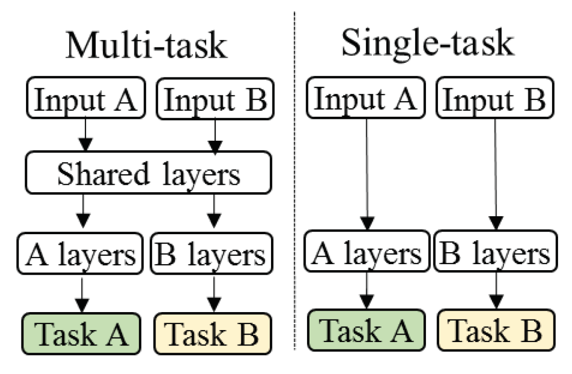
These ML algorithms learn one model for each training dataset. The ML approach capable of learning models for several ML datasets (ML tasks) in parallel while using a shared representation is Multi-task learning (MTL) [
76]. The idea is to use what was learned from one dataset to help learn other tasks better. More specifically, in single-task neural networks, backpropagation algorithm is used to minimize a single loss function, and single neuron provides the final output. MTL, on the other hand, involves the minimization of a joint loss function (e.g., weighted sum of the binary cross-entropies of all tasks) and learning shared representations over all tasks (see
Figure 1). The specific MTL architecture was similar to the MLP architecture (
https://repo.ijs.si/martingjoreski/cognitive-load/-/blob/master/MTL.png). It contains two shared-hidden layers of size 512 units, one task-specific layer of size 32 units, and two task-specific sigmoid units that output the final predictions.
Both for the MTL and MLP architectures, ReLU activation units [
77] were used in the hidden layers, which speeds up the training process compared to other activation layers (e.g., tanh). To avoid overfitting, L2 regularization and dropout were used. The training of the networks was fully supervised, by back propagating the gradients through all the layers. The parameters were optimized by minimizing the binary cross-entropy loss function using the Adam optimizer. The models were trained with a learning rate of
and a decay of
. The batch size was set to 32, and the number of training epochs was set to 50.
5.3. Experimental Setup
Leave-one-session-out evaluation techniques were used in all ML experiments. This means that the data of one session were used as a test data, and the rest of the data were used for training and tuning the ML models. In the CogLoad dataset, there is only one session per participant, thus the models are participant-independent. In the Snake dataset, there is more than one session for some participants, thus the models are participant-dependent.
For each ML algorithm, parameter tuning was performed using the following procedure: parameter settings were randomly sampled from distributions predefined by an expert. Next, models were trained with the specific parameters and then evaluated using internal k-fold cross-validation on the training data. The best performing model from the internal k-fold cross-validation was used to classify the test data. This tuning procedure was performed as many times as there were sessions in the specific experimental dataset. Additionally, the evaluation was repeated five times to account for the randomness present in the learning (e.g., Random Forest) and the tuning (e.g., the random parameter sampling) of the ML models.
For the CogLoad dataset, the ML task was the classification of rest vs. task segments. For the Snake dataset, the ML task was the classification of easy vs. hard segments. The rest periods were not recorded in the Snake dataset, thus rest vs. task classification is not possible. Additionally, for the Snake dataset, the segments with medium difficulty were not used in the ML analysis following the studies by Rissler et al. [
78] and Maier et al. [
79], in which only the top 20% and the lowest 20% of the data points were considered for the classification task. The data points that fall in between were discarded.
Table 7 presents the size of the experimental datasets after the labeling. Each instance represents a 30-second segment labeled with a “High” or “Low” difficulty.
The averaged results for a binary classification problem are presented in
Table 8. All models were dataset-specific, except for the MTL model, which is a joint model for the two datasets. The last three columns present the accuracy of the ML models built using selected features in combination with raw features (without any normalization), normalized features (min-max normalization), and standardized features. The three columns before that present the accuracy of each ML model built using all features in combination with raw features, normalized features, or standardized features.
7. Conclusions and Future Work
This study presented two datasets of multimodal data sensed with a commodity wearable device, while the participants were exposed to a varying cognitive load. To the best of our knowledge, these are the first datasets that include such rich sensor data augmented with the information on the personality traits of the participants. The experimental setup in which the datasets were collected included a variety of cognitive tasks performed on a smartphone and on a PC. We also presented an analysis of the psychological data in relation to the subjective cognitive load (NASA-TLX) and the objective cognitive load measures, revealing potentially significant relationships. For example, we found that people who rank high in emotionality find tasks physically more demanding and have higher heart rates during task solving (and vice versa). In addition, there was evidence that people who scored low on humility may report higher performance scores, but are very susceptible to cognitive load. Furthermore, we present baseline ML models for recognizing task difficulty. The person-independent models on the CogLoad dataset achieved an accuracy of 68.2%, while the person-dependent models on the Snake dataset achieved an accuracy of 82.3%. These results are in line with related work that uses more sophisticated lab-based measurement equipment. The proposed multi-task learning (MTL) neural network outperformed the single-task neural network (a Multi-layer perceptron; MLP) by simultaneously learning from the two datasets. The datasets will be made publicly available to advance the field of cognitive load inference using commercially available devices.
Our next step will be to build ML models that combine both the psychological and physiological data for inferring cognitive load [
89]. Personality grouping shows differences between people on a more fundamental level, and these differences can be expressed physiologically. Grouping can be made either through unsupervised learning, i.e., clustering, or expert techniques (e.g., making groups on dominant dimensions). Finding ‘noisy’ participants is important as well. One-sixth of participants give false answers to psychological questionnaires [
90]. For example, in our data, these individuals could be filtered out through the honesty-humility trait score. Making separate models for different groups is, therefore, viable as well. This should improve our current results as well as strengthen our vision for more interdisciplinary research on cognitive phenomena.

 ,
, 


