Reliability-Enhanced Camera Lens Module Classification Using Semi-Supervised Regression Method

Abstract

Artificial intelligence has become the primary issue in the era of Industry 4.0, accelerating the realization of a self-driven smart factory. It is transforming various manufacturing sectors including the assembly line for a camera lens module. The recent development of bezel-less smartphones necessitates a large-scale production of the camera lens module. However, assembling the necessary parts of a module needs much room to be improved since the procedure followed by its inspection is costly and time-consuming. Consequently, the collection of labeled data is often limited. In this study, a reliable means to predict the state of an unseen camera lens module using simple semi-supervised regression is proposed. Here, an experimental study to investigate the effect of different numbers of training samples is demonstrated. The increased amount of data using simple pseudo-labeling means is shown to improve the general performance of deep neural network for the prediction of Modulation Transfer Function (MTF) by as much as 18%, 15% and 25% in terms of RMSE, MAE and R squared. The cross-validation technique is used to ensure a generalized predictive performance. Furthermore, binary classification is conducted based on a threshold value for MTF to finally demonstrate the better prediction outcome in a real-world scenario. As a result, the overall accuracy, recall, specificity and f1-score are increased by 11.3%, 9%, 1.6% and 7.6% showing that the classification of camera lens module has been improved through the suggested semi-supervised regression method.

1. Introduction

The recent development of bezel-less smartphones necessitates a large-scale production of the camera lens module before it is ready for use in the assembly stage. A camera lens module, which is normally placed at the front and back of a smartphone, consists of several spherical and aspheric lens stacked vertically inside a customized barrel [1]. Figure 1 illustrates the exploded view of an ordinary camera lens module. The determination of a well-made camera lens module relies upon the combination of the upright lens configuration as well as several external factors including barrel thickness and lens diameter [1]. With the number of factors that influence the performance of a module reaching a few hundred, it is important to understand which ones are more significant in its overall performance. Just as importantly, one must figure out the future modification of the factors to achieve a higher yield rate on the production of camera modules.

One of the key factors, lens arrangement, directly determines the amount and the focus of light hitting the sensor. The main purpose of stacking multiple lenses in the right arrangement is to reduce the light from a large screen to fit the small size of the sensor. Modulation Transfer Function (MTF), a continuous variable that indicates the definition of the image created by the focused light, is a commonly used measure to compare the performance of optical systems. In definition, MTF is the magnitude response of an optical system to sinusoids of various spatial frequencies. In this study, MTF is used as the target variable to represent the quality of a lens module.

Despite the huge impact on the quality, the traditional method to find the right arrangement is to simply turn each lens one at a time by a certain amount of degrees manually until the requirement is met. The procedure includes multiple inspections of every 10 products sampled when an issue is discovered from already manufactured products. By plotting the MTF curve of each product, either lens re-arrangement or thickness modification of a spacer and the lenses is made. Modifying the thickness of a spacer and lenses is done if the vertices are concentrated at a wrong spot. On the other hand, the lens re-arrangement is conducted when the vertex of MTF curve is lower than a threshold value, which is usually the most common case. It is a more preferred option since it is easier to do than the other. The lenses are normally rotated 45 degrees clockwise from their original positions. This kind of task is not only time-consuming but it also does not guarantee a better result after it has been conducted. In addition, no reliable way to screen the effect of slight modification in real-time exists, implying that one sample can be tested only after it is completely capped inside a barrel. Such repetitive and tedious operation necessitated an automated system to foresee the outcome of products without the assembly.

Over the past few years, deep learning has emerged as a powerful tool in many engineering fields such as image processing, voice recognition and natural language processing, triggered by the advent of a fast computing hardware, e.g., GPU [2]. Its wide range of applicability has brought a new trend in both research and industrial sectors of our society, leading to the development of the popular deep neural network (DNN), convolutional neural network (CNN), recurrent neural network (RNN), and autoencoder [2]. DNN is simply an extension of the ordinary neural network with a single hidden layer, and a simplified model representation of the complex human brain. It is often referred to as a multi-layered perceptron network that is capable of understanding the non-linear nature of high-dimensional feature space. This is due to the non-linear activation function applied after the nodes of the hidden networks. Despite its huge potential as a non-linear function approximator, one of the limitations of DNN is that it normally requires a sufficient amount of data to provide reliable output. Though no strict guideline is established for the right amount of training data; since it varies depending on the type of problem to be solved, a general rule of thumb is to have the number of data at least ten times the feature dimension [3]. However, obtaining big data is often limited due to the lack of available infrastructure, which raises demand for a method to create a similar training set and provide it with a reasonable label. In the manufacturing industry, the labeling of acquired data is often very restricted since it is only possible after the actual manufacturing of products, which often requires much resource and time. Such restriction led to the development of various methods that artificially provide labels to those data without the need for an actual experiment. Most previous studies, however, focus on the pseudo-labeling of categorical data. Semi-supervised regression (SSR), a method to pseudo-label a continuous variable has so far been limited in real-world applications due to the complexity of understanding the existing algorithms that provide a suitable regression output.

In this study, a simple but effective SSR coupled with simple random sampling (SRS) for the generation of synthetic data is proposed to boost the overall regression performance of DNN. Then, camera lens module classification is performed based on the improved regression model enhancing the reliability of the classification result. To the best of our knowledge, no prior work has ever attempted a deep learning-based approach to the classification of the camera lens module. The module is classified as either ‘satisfactory’ or ‘unsatisfactory’ based on the regression result that is improved using SSR. The rest of the paper is broken down as follows. Section 2 provides an overview of related work, whilst Section 3 details the proposed methodology. The experimental result is discussed in Section 4.1, and finally, the paper is concluded in Section 5.

2. Related Work

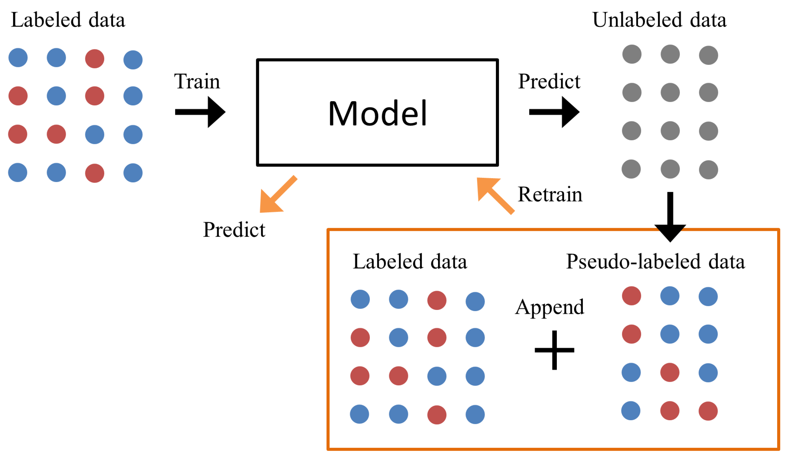
2.1. Semi-Supervised Learning

Semi-supervised learning is a branch of machine learning which utilizes both labeled and unlabeled data to improve the overall generalization performance of a model. It has earned a tremendous amount of attention in various fields of research such as bioscience, material science, and manufacturing industry where the actual testing of unseen data is time-consuming and labor intensive [4]. Due to its boost in popularity, despite its abstruse nature, several approaches including expectation-maximization, split-learning, graph-based methods, co-training, and self-training have been developed [5]. However, none of these approaches is easily comprehensible to non-experts, especially those practitioners of the deep learning community who do not know the physical meaning of or statistics behind the data they deal with. Hao et al. [6] used a clustering algorithm, Dirichlet process mixture model (DPMM) to provide pseudo-class labels for unlabeled data. It has shown to be effective since DPMM is a non-parametric clustering algorithm and is thus able to figure out the unknown background classes from the unlabeled ones. Even if no labels are given, samples can be grouped based on their similarities, providing them with pseudo labels. To improve the performance, a pre-trained DNN model is first constructed using all the training data with the pseudo-labels. Then, a second DNN model is introduced by taking all the layers except the last one from the pre-trained model. The new model is then fine-tuned using only the true class labels.

It gets trickier in a regression problem because the dependent variable is no longer a discrete categorical value and is thus difficult to be categorized into groups. To make the matter worse, most studies deal with semi-supervised classification (SSC) rather than SSR as the former is deemed a more general case [7]. As a result, several SSR algorithms, despite the efficiency, is hard to implement. Similar algorithms such as semi-supervised support vector regression (SS-SVR) [8], COREG [9], CoBCReg [10], semi-supervised kernel regression (SSKR) [11], spectral regression [12] are proposed but only a few of them have been used in real-world applications due to the limited applicability, i.e., highly dependent on data type [7]. Cases of previous literature regarding SSR and its use on real-world applications are tabulated in

Table 1. Previous studies regarding SSR and its real world applications.

Type	SSR Method	Algorithm	Real-World Applications	Publications
Non-parametric	Semi-supervised co-regression	COREG	Real world dataset (UCI, StatLib), Sunglasses lens	[14,15]
		CoBCReg	N/A	[16]
		SAFER	Real world dataset (NTU)	[17]
	Semi-supervised kernel regression	SS-SVR	Semiconductor manufacturing,	[18,19,20,21,22]
			Soft-sensing process,
			Benchmark (Boston, Abalone, etc.),
			Hyperspectral satellite images,
			MERIS,
			Corn,
			Real world dataset (Delve, TSDL, StatLib)
		KRR	Real world dataset (Boston housing, California housing, etc.),	[23,24,25]
			IRIS, Colon cancer, Leukemia,
			Real world dataset (Boston, kin32fh)
		POKR	Real world dataset	[26]
	SSR via graph regularization	GLR	Geographical photo collections,	[27,28]
			Delve Census, Orange juice
		Hessian Regularization	Real world dataset	[29]
		Parallel Field Regularization	Temperature, Moving hands	[30]
		Spectral Regression	MNIST, Spoken letter	[31]
	Local linear SSR	LLSR	Real world dataset	[32]
	Semi-supervised Gaussian process regression	SSMTR	N/A	[33]
Parametric	Semi-supervised linear regression	SSRM	German	[16]

. To circumvent the issue, this study utilizes the self-labeling method [13], which is simple and effective to enhance the overall regression performance on data collected from sensors at a production line.

2.2. Machine Learning Algorithms

In this section, machine learning algorithms used for pseudo-labeling are briefly explained.

• XGBoost
  XGBoost [34] is a type of ensemble as well as a boosting algorithm that combines multiple decision trees. It is a scalable version of Gradient Boosting introduced by Friedman et al. [35]. It adjusts the weights of the next observation based on the previous one. The algorithm generally shows strong predictive performance and it has earned much popularity at the Kaggle competitions by achieving high marks in numerous machine learning tasks.
• Random Forest
  Random Forest [36] is a bagging algorithm that uses an ensemble of decision trees. It effectively decreases the variance in the prediction by generating various combinations of training data. Its major advantage lies in the diversity of decision trees as variables are randomly selected. It is frequently used for both classification and regression tasks in machine learning.
• Extra Trees
  Extra trees [37] is a variant of random forest which is a popular bagging algorithm based on the max-voting scheme. extra trees are made up of several decision trees in which there are multiple root nodes, internal nodes, and leaf nodes. For each decision tree, a different bootstrapped data set is used. It should also be noted that for bootstrapping, all samples are eventually used because they are selected without replacement. At each step in building a tree and forming a node, a random subset of variables is considered resulting in a wide variety of trees. At the same time, a random value is selected for each variable under consideration leading to more diversified trees and fewer splitters to evaluate. The diversity and smaller tree depths are what make extra trees more effective than Random Forest as well as individual decision trees. Once various decision trees are established, a test sample would run down each decision tree to deliver outputs. The most frequent output will be provided as the final label to the test sample as the result of the max-voting scheme.
• Multilayer Perceptron
  Multilayer perceptron [38] is a feed-forward neural network composed of multiple layers of perceptron. It is usually differentiated from DNN by the number of hidden layers. It utilizes a non-linear activation function to learn the non-linearity of input features.

3. Methodology

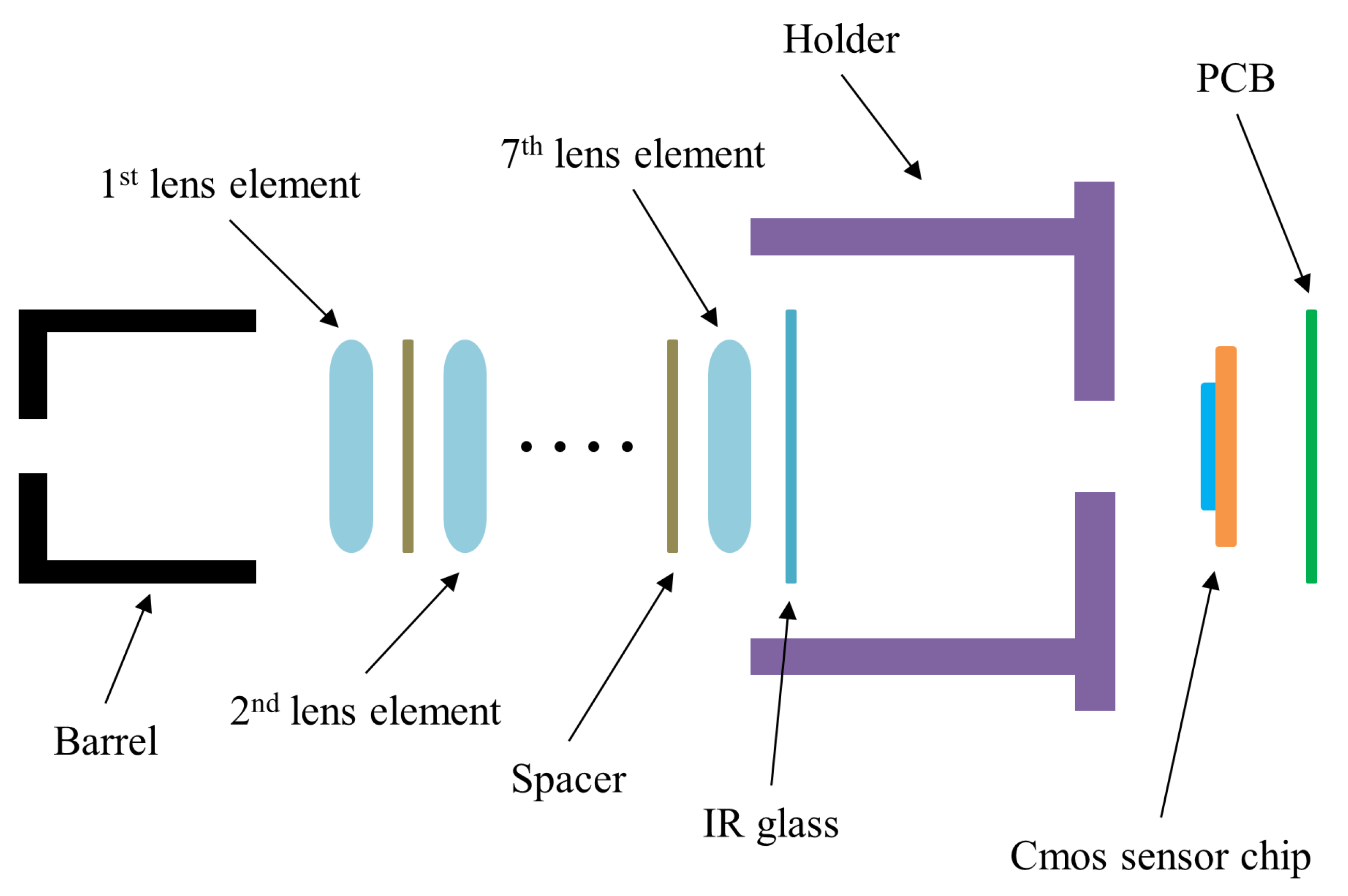
3.1. Dataset Preprocessing

Raw data goes through a series of steps, called pre-processing so that it becomes readily actionable, or structured as in the view of a data scientist. One example of this includes the labeling of the MTF outcome that should be assigned with either ‘0’ if the value is above a threshold or ‘1’ otherwise. The labels indicate ‘satisfactory’ and ‘unsatisfactory’ status of products respectively. The class-labeled data is only used for classification. Then, the input variables are normalized to values within range from 0 to 1. In this study, camera lens module data obtained by various sensors is used as an input.

Table 2. Independent variables as inputs of DNN.

Input Variables
Process condition	Lens properties			Barrel			Spacer
Lens angle	Outer diameter	Inner diameter	Roundness	Thickness	Concentricity	Inner diameter	Thickness

shows the types of input variables used for training, while the output variable is MTF.

However, the number of collected data samples from the sensors is less than a few hundred, making it extremely challenging to predict the output. To solve this issue, the unlabeled data set is synthesized using SRS on each input variable. SRS takes samples of each element of the variables based on equal probability distribution [39]. Then, they are given labels following the simple semi-supervised pseudo-labeling method as illustrated in Figure 2.

First, a model is selected to train the raw data set. The best performing model on the raw data is then used to assign pseudo-labels on the synthesized data. For selecting a model, we take account of only machine learning algorithms because they are known to be much more suitable with small amount of data. Of the various algorithms (Random Forest, XGBoost, Gradient Boost, K-nearest Neighbor, Extra Trees, and Multi-layer Perceptron), the selected model is Extra Trees since it showed the best performance on the raw data. Lastly, the newly labeled data is shuffled well with the raw data, thus leading to a better performing model with an increased number of data samples. The disadvantage of this simplified pseudo-labeling method is that the selection of the model determines the quality of synthesized data labeling. Moreover, the error might add up because of an increase in the number of data samples. Therefore, the optimal number of samples for the best prediction is determined by an exhaustive method, where 10 different data sets with the number of samples increasing in order are tested respectively.

Table 3. Raw data and nine data sets augmented by Simple Random Sample.

Sampling Method	Training Data Set	Number of Sampled Data
Simple Random Sample (SRS)	1	128
	2	256 (multiples, 2×)
	3	384 (multiples, 3×)
	4	512 (multiples, 4×)
	5	640 (multiples, 5×)
	6	768 (multiples, 6×)
	7	1280 (multiples, 10×)
	8	2560 (multiples, 20×)
	9	5120 (multiples, 40×)
	10	10,240 (multiples, 80×)

is a list of the aforementioned data sets with each corresponding number of samples. Furthermore, 5-fold cross-validation is implemented to ensure a more generalized test result and to avoid overfitting. The performance metrics used for the regression task are RMSE, MAE, and R-squared. For the computation, we used GeForce RTX 2080 (NVIDIA, Santa Clara, California, CA, USA, 1993) that was used to run Python 3.5.3 and Tensorflow 1.13.1.

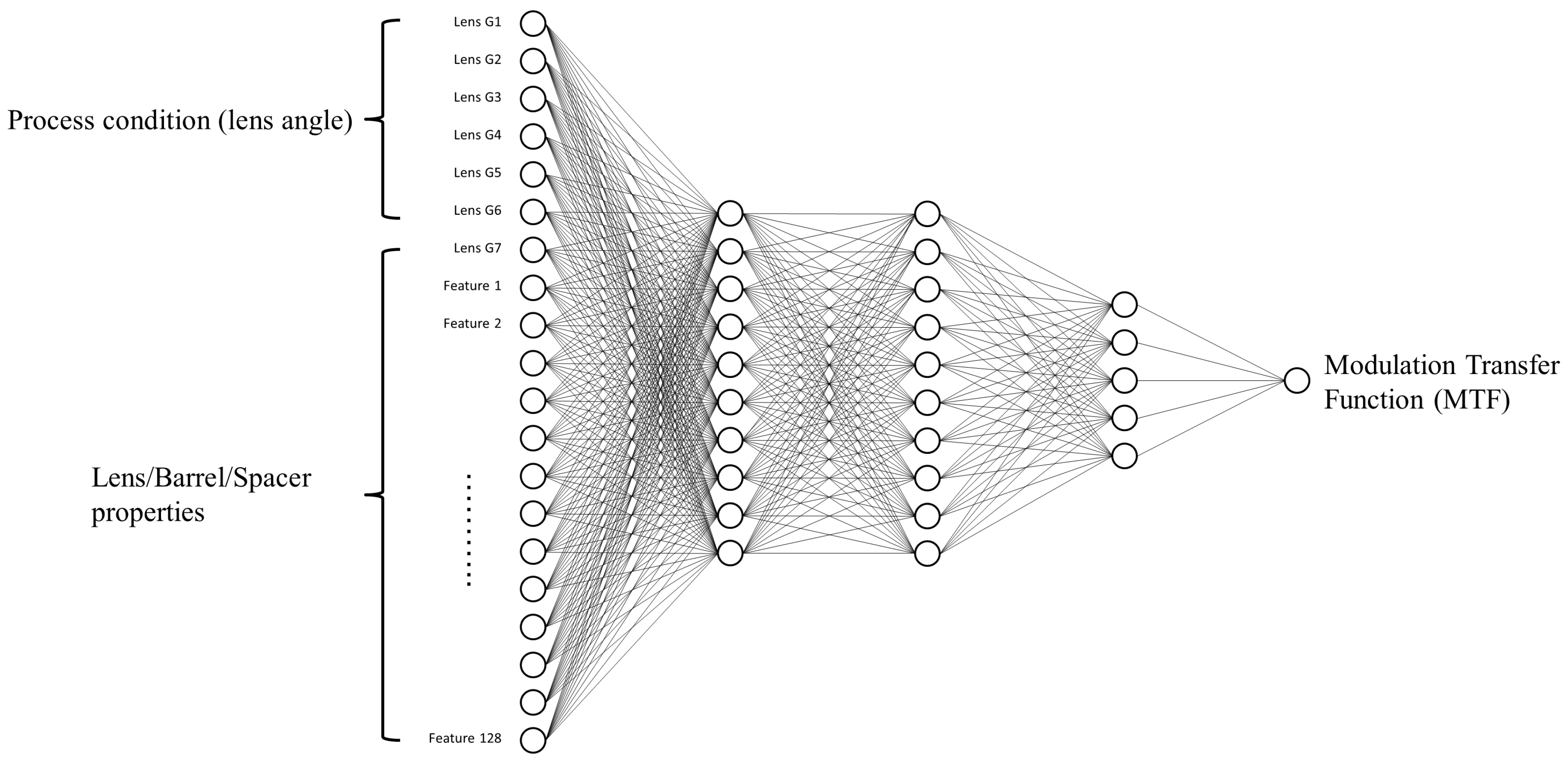
3.2. Deep Learning Architecture

Followed by data pre-processing, a DNN model as shown in Figure 3 is constructed to predict the MTF. The structure of the model is determined in a heuristic fashion. There are three hidden layers, each of which has 10 nodes respectively. The final node constitutes a single node for outputting a regression result. For the training, Adam optimizer, ReLU activation function and Xavier initializer are used. ReLU activation function is applied after every multiplication of weight plus bias but is omitted at the final layer. The objective function is the Mean Squared Error (MSE), which calculates the mean of the squared difference between the target value and each batch samples. The optimal hyper-parameters including learning rate, iteration and batch size are discovered using a small portion of training data (15%) based on grid-search. Early stopping is implemented to break the training procedure.

Table 4. Top 5 results with varying hyper-parameters.

Learning Rate	Iteration	Batch Size	Layer	Number of Samples	Validation Set	RMSE	MAE	${\mathit{R}}^{\mathbf{2}}$
3 × ${10}^{-4}$	3,125,550	32	[10, 10, 5]	384	Val 5	5.584	5.582	0.678
4 × ${10}^{-6}$	119,400	16	[10, 10, 5]	128	Val 2	5.705	5.000	0.738
3 × ${10}^{-4}$	3,349,350	64	[10, 10, 5]	768	Val 5	5.861	5.170	0.645
2 × ${10}^{-5}$	4,336,650	256	[10, 10, 5]	1280	Val 2	5.880	5.630	0.720
2 × ${10}^{-5}$	4,282,800	256	[10, 10, 5]	768	Val 2	6.120	5.420	0.698

shows the top 5 results when different hyper-parameters are applied for the training of the model.

Once the hyper-parameters are optimized, the best regression result is attained and the optimal number of samples is determined, the next step is to implement classification using class-labeled data. The deep learning model is similar to the one used for the regression but the objective function as well as the activation function used at the final layer. Since it is a multi-class classification problem, categorical cross-entropy loss is minimized for optimization and softmax function is applied at the final layer of the DNN. Here, an area under the ROC curve (AUC) is calculated to see if there is any improvement by comparing the classification results between the augmented and the raw data.

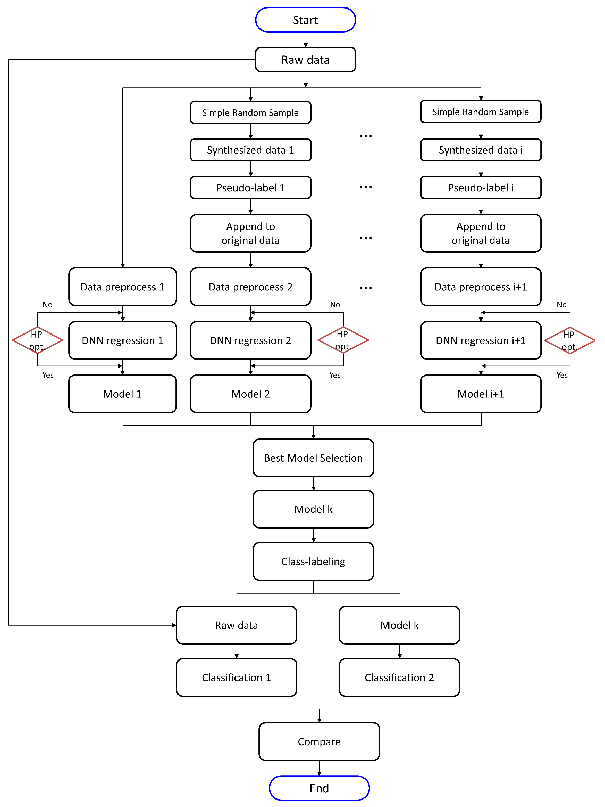
3.3. Experimental Workflow

The overall procedure is illustrated and summarized in the flowchart below (Figure 4). ‘HP opt’ stands for hyper-parameter optimization. The overall workflow is divided largely into two parts. The first part is to improve the general regression performance by training additional data in a semi-supervised manner. The second part is to make classification on the raw and the augmented models. To convert into a binary classification task, it is necessary to switch the continuous target variable into a discrete variable with either ‘0’ or ‘1’ labels based on the user-defined discrimination threshold value of MTF, and it is done after an optimized regression model has been discovered. The class-labeling process is described in Section 3.1. Optimizing the regression model is necessary because the classification accuracy is directly dependent on how closely the established regression model can predict the output. Getting into more details of the first part, given the raw data, the procedure splits into 10 branches in which different data sets from Table 3 are processed to give the best performing model in terms of regression. For synthesizing different data sets as listed in Table 3, simple random sampling on raw data is conducted. The sampled data are then appended to the raw data to make up augmented data sets. They are then given pseudo labels by extra trees regressor. Subsequently, the type of regression model used is DNN with the architecture as specified in Section 3.2 Each regression model is tested by 5-fold cross-validation. As for the second part, the aforementioned class-labeling is implemented, followed by training of a similar network with the selected model k. Finally, it is then compared with the model using raw data for the classification task.

4. Result and Discussion

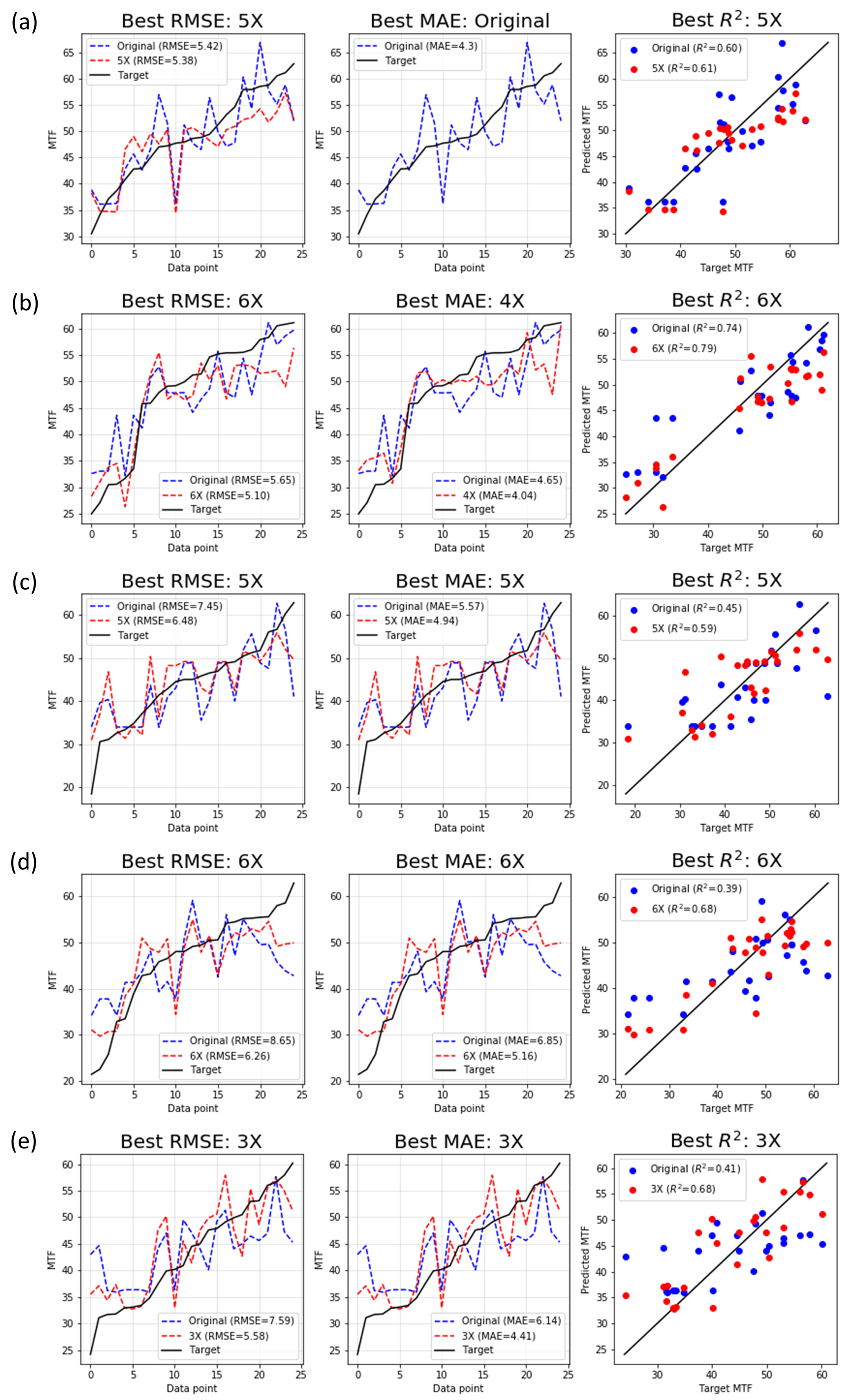
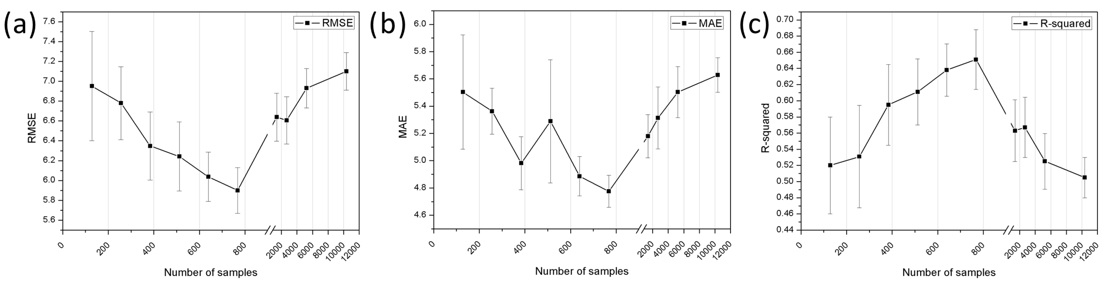
4.1. Regression Performance

Prediction of MTF is plotted in Figure 5. Since the test set is split into five subsets, the regression plot for each test set are shown from top to bottom.

Even though the best performing data set for all performance metrics tends to vary as the test set is changed, the overall regression result improves as the number of samples is increased. This is shown by the prediction curve in the red dotted line that is much more generalized than the blue dotted line. Figure 6 shows the average values of validation results presented in Figure 5 in terms of RSME, MAE, and $R^2$. It shows that it is best to use 768 samples for training to get the least RMSE, MAE and the highest $R^2$, which in this case are 5.89, 4.78 and 0.65 respectively.

The result implies that the performance increases by 18%, 15% and 25% for each performance metric when more training data is used. However, the plots also show that the performance begins to degrade at the number of samples of 768. This is because the first model for pseudo-labeling of the synthesized data is not the best, thus the pseudo labels should bear an error indispensably. In addition, through SRS for generating synthetic data, infeasible samples may have been generated. This implies that additional training data with error should be used only in a limited amount. To demonstrate that the data augmentation through pseudo labeling brings improvement in the general regression performance, the evaluation metrics are also measured for several other promising machine learning algorithms as shown in

Table 5. Regression results comparing with the proposed method. Better results are highlighted in bold.

Metric	SVM	Random Forest	Gradient Boosting	XGBoost	Proposed Method
RMSE	9.83	6.19	6.19	5.98	5.89
MAE	6.84	4.53	4.59	4.34	4.78
$R^2$	0.25	0.58	0.58	0.61	0.65

. Though it does not excel in every aspect, our proposed model shows the best result overall. The hyper-parameters for each machine learning algorithms have been heuristically optimized as follows: Support Vector Machine (kernel = ’rbf’ and regularization parameter C = 5.0), Random Forest (number of trees = 100 and max depth = 2), Gradient Boosting (number of boosting stages = 100, learning rate = 0.1 and max depth = 5), XGBoost (learning rate = 0.3, max depth = 6 and L2 regularization term on weights = 1).

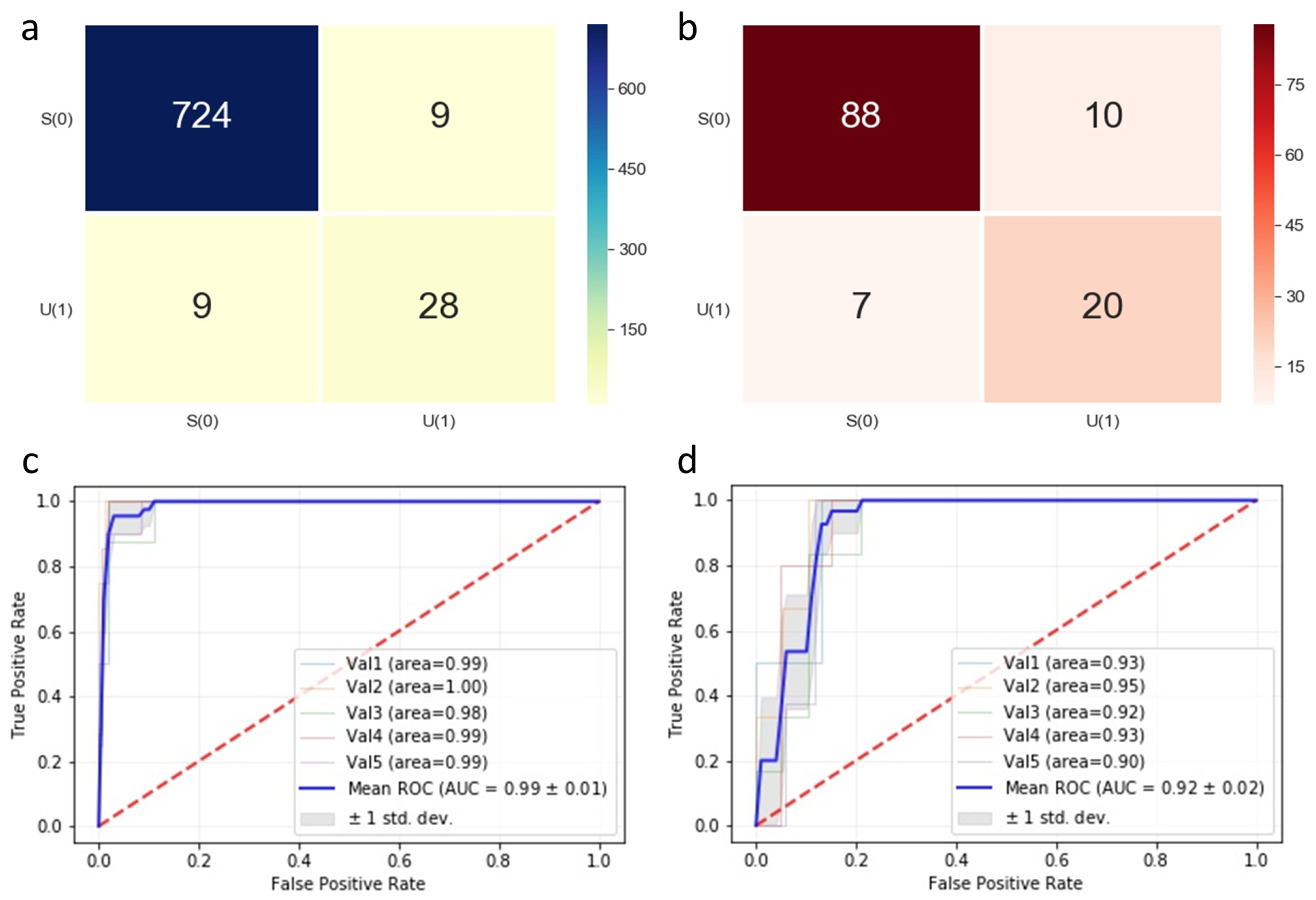
4.2. Classification Performance

The effectiveness of increasing the number of training data through a pseudo-labeling is also apparent in the classification task.

Table 6. Accuracy, recall, specificity and f1-score for augmented and raw data.

Data Type	Accuracy	Recall	Specificity	F1-Score
Augmented	97.7%	98.8%	75.7%	98.8%
Raw	86.4%	89.8%	74.1%	91.2%

shows accuracy, recall, specificity and f1-score for the augmented and the raw data. The overall accuracy, recall, specificity and f1-score increase by 11.3%, 9%, 1.6% and 7.6% at best when more data is used to train a deep learning model implying that the proposed method would most likely be correct on camera lens module classification and is more reliable in terms of prediction. The better f1-score provides more reliability to the conclusion because the test sets are class imbalanced and f1-score is a more suitable measure for such a case. The rates are calculated based on the summed confusion matrices for five test sets shown in Figure 7. Looking at the ROC curves, AUCs generally get higher when the augmented data is used for training. This implies that the constructed model is more capable of distinguishing between the two classes. Therefore, it is now better at predicting zeros as zeros and ones as ones.

5. Conclusions

Collecting data is often very restricted due to the lack of infrastructure. It is even more restrictive when labeling data is possible only through the manufacturing of products. The goal of this paper is to demonstrate the effectiveness of making a prediction through a simple but effective method when there is small amount of labeled data available on-hand. In this study, a semi-supervised regression (SSR) coupled with simple random sampling (SRS) for the generation of synthetic data is proposed to boost the overall regression performance of DNN. Then, camera lens module classification is performed based on the improved regression model enhancing the reliability of the classification result. The performance of the proposed model is validated on five different test sets for both raw and augmented models. The proposed scheme shows that the regression performance increases by 18%, 15%, and 25% while the classification performance does by 11.3%, 9%, 1.6%, and 7.6% at best, achieving 97.7% accuracy, 98.8% recall, 75.7% specificity, and 98.8% f1-score on average. This result shows that the classification performance which is heavily influenced by the discrimination threshold value of MTF is increased with the help of improved regression. Although the overall performance has improved, it is shown in the result section of regression that it begins to degrade at some point. This is due to the error in the pseudo label and the lack of raw data making it challenging to figure out the true distribution of the data. One possible alternative to SRS would be to try some other sampling methods given that the distributions of the input variables are known. Another interesting approach would be to iterate the pseudo-labeling process a few more times until the performance ceases to get better.

References

1. Steinich, T.; Blahnik, V. Optical design of camera optics for mobile phones. Adv. Opt. Technol. 2012, 1, 51–58. [Google Scholar] [CrossRef]
2. Hatcher, W.G.; Yu, W. A survey of deep learning: Platforms, applications and emerging research trends. IEEE Access 2018, 6, 24411–24432. [Google Scholar] [CrossRef]
3. Gheisari, M.; Wang, G.; Bhuiyan, M.Z.A. A survey on deep learning in big data. In Proceedings of the 2017 IEEE International Conference on Computational Science and Engineering (CSE) and IEEE International Conference on Embedded and Ubiquitous Computing (EUC), Guangzhou, China, 21–24 July 2017; IEEE: New York, NY, USA, 2017; Volume 2, pp. 173–180. [Google Scholar]
4. Zhang, X.; Yin, J.; Zhang, X. A semi-supervised learning algorithm for predicting four types MiRNA-disease associations by mutual information in a heterogeneous network. Genes 2018, 9, 139. [Google Scholar] [CrossRef] [PubMed] [Green Version]
5. Chandna, P.; Deswal, S.; Pal, M. Semi-supervised learning based prediction of musculoskeletal disorder risk. J. Ind. Syst. Eng. JISE 2010, 3, 291–295. [Google Scholar]
6. Wu, H.; Prasad, S. Semi-supervised deep learning using pseudo labels for hyperspectral image classification. IEEE Trans. Image Process. 2017, 27, 1259–1270. [Google Scholar] [CrossRef] [PubMed]
7. Kostopoulos, G.; Karlos, S.; Kotsiantis, S.; Ragos, O. Semi-supervised regression: A recent review. J. Intell. Fuzzy Syst. 2018, 35, 1483–1500. [Google Scholar] [CrossRef]
8. Wang, X.; Fu, L.; Ma, L. Semi-supervised support vector regression model for remote sensing water quality retrieving. Chin. Geogr. Sci. 2011, 21, 57–64. [Google Scholar] [CrossRef]
9. Zhou, Z.H.; Li, M. Semi-Supervised Regression with Co-Training. IJCAI 2005, 5, 908–913. [Google Scholar]
10. Hady, M.F.A.; Schwenker, F.; Palm, G. Semi-supervised Learning for Regression with Co-training by Committee. In International Conference on Artificial Neural Networks; Springer: Berlin, Germany, 2009; pp. 121–130. [Google Scholar]
11. Wang, M.; Hua, X.S.; Song, Y.; Dai, L.R.; Zhang, H.J. Semi-supervised kernel regression. In Proceedings of the Sixth International Conference on Data Mining (ICDM’06), Hong Kong, China, 18–22 December 2006; IEEE: New York, NY, USA, 2006; pp. 1130–1135. [Google Scholar]
12. Cai, D. Spectral Regression: A Regression Framework for Efficient Regularized Subspace Learning. Ph.D. Thesis, University of Illinois at Urbana-Champaign, Urbana, IL, USA, 2009. [Google Scholar]
13. Lee, D.H. Pseudo-label: The simple and efficient semi-supervised learning method for deep neural networks. In Workshop on Challenges in Representation Learning; ICML: Atlanta, GA, USA, 2013; Volume 3, p. 2. [Google Scholar]
14. Zhou, Z.H.; Li, M. Semisupervised regression with cotraining-style algorithms. IEEE Trans. Knowl. Data Eng. 2007, 19, 1479–1493. [Google Scholar] [CrossRef] [Green Version]
15. Sun, X.; Gong, D.; Zhang, W. Interactive genetic algorithms with large population and semi-supervised learning. Appl. Soft Comput. 2012, 12, 3004–3013. [Google Scholar] [CrossRef]
16. Ng, M.K.; Chan, E.Y.; So, M.M.; Ching, W.K. A semi-supervised regression model for mixed numerical and categorical variables. Pattern Recognit. 2007, 40, 1745–1752. [Google Scholar] [CrossRef] [Green Version]
17. Li, Y.F.; Zha, H.W.; Zhou, Z.H. Learning safe prediction for semi-supervised regression. In Proceedings of the Thirty-First AAAI Conference on Artificial Intelligence, San Francisco, CA, USA, 4–9 February 2017; AAAI: San Francisco, CA, USA, 2017. [Google Scholar]
18. Kang, P.; Kim, D.; Cho, S. Semi-supervised support vector regression based on self-training with label uncertainty: An application to virtual metrology in semiconductor manufacturing. Expert Syst. Appl. 2016, 51, 85–106. [Google Scholar] [CrossRef]
19. Ji, J.; Wang, H.; Chen, K.; Liu, Y.; Zhang, N.; Yan, J. Recursive weighted kernel regression for semi-supervised soft-sensing modeling of fed-batch processes. J. Taiwan Inst. Chem. Eng. 2012, 43, 67–76. [Google Scholar] [CrossRef]
20. Zhu, X.; Goldberg, A.B. Kernel regression with order preferences. In Proceedings of the National Conference on Artificial Intelligence; AAAI Press: Palo Alto, CA, USA, 1989; MIT Press: Cambridge, MA, USA, 1932; Volume 22, p. 681. [Google Scholar]
21. Camps-Valls, G.; Munoz-Mari, J.; Gómez-Chova, L.; Calpe-Maravilla, J. Semi-supervised support vector biophysical parameter estimation. In Proceedings of the IGARSS 2008—2008 IEEE International Geoscience and Remote Sensing Symposium, Boston, MA, USA, 7–11 July 2008; IEEE: New York, NY, USA, 2008; Volume 3, p. III-1131. [Google Scholar]
22. Xu, S.; An, X.; Qiao, X.; Zhu, L.; Li, L. Semi-supervised least-squares support vector regression machines. J. Inf. Comput. Sci. 2011, 8, 885–892. [Google Scholar]
23. Cortes, C.; Mohri, M. On transductive regression. In Advances in Neural Information Processing Systems; NeurIPS: San Diego, CA, USA, 2007; pp. 305–312. [Google Scholar]
24. Angelini, L.; Marinazzo, D.; Pellicoro, M.; Stramaglia, S. Semi-supervised learning by search of optimal target vector. Pattern Recognit. Lett. 2008, 29, 34–39. [Google Scholar] [CrossRef] [Green Version]
25. Chapelle, O.; Vapnik, V.; Weston, J. Transductive inference for estimating values of functions. In Advances in Neural Information Processing Systems; NeurIPS: San Diego, CA, USA, 2000; pp. 421–427. [Google Scholar]
26. Brouard, C.; D’Alché-Buc, F.; Szafranski, M. Semi-supervised Penalized Output Kernel Regression for Link Prediction. In Proceedings of the 28th International Conference on Machine Learning (ICML 2011), Bellevue, WA, USA, 28 June–2 July 2011; ICML: Atlanta, GA, USA, 2011; pp. 593–600. [Google Scholar]
27. Xie, L.; Newsam, S. IM2MAP: Deriving maps from georeferenced community contributed photo collections. In Proceedings of the 3rd ACM SIGMM International Workshop on Social Media, Scottsdale, AZ, USA, 30 November 2011; ACM: New York, NY, USA, 2011; pp. 29–34. [Google Scholar]
28. Doquire, G.; Verleysen, M. A graph Laplacian based approach to semi-supervised feature selection for regression problems. Neurocomputing 2013, 121, 5–13. [Google Scholar] [CrossRef]
29. Kim, K.I.; Steinke, F.; Hein, M. Semi-supervised regression using Hessian energy with an application to semi-supervised dimensionality reduction. In Advances in Neural Information Processing Systems; NeurIPS: San Diego, CA, USA, 2009; pp. 979–987. [Google Scholar]
30. Lin, B.; Zhang, C.; He, X. Semi-supervised regression via parallel field regularization. In Advances in Neural Information Processing Systems; NeurIPS: San Diego, CA, USA, 2011; pp. 433–441. [Google Scholar]
31. Cai, D.; He, X.; Han, J. Semi-Supervised Regression Using Spectral Techniques; Technical Report UIUCDCS-R-2006-2749; Computer Science Department, University of Illinois at Urbana-Champaign: Urbana, IL, USA, 2006. [Google Scholar]
32. Rwebangira, M.R.; Lafferty, J. Local Linear Semi-Supervised Regression; School of Computer Science Carnegie Mellon University: Pittsburgh, PA, USA, 2009; Volume 15213. [Google Scholar]
33. Zhang, Y.; Yeung, D.Y. Semi-supervised multi-task regression. In Joint European Conference on Machine Learning and Knowledge Discovery in Databases; Springer: Berlin, Germany, 2009; pp. 617–631. [Google Scholar]
34. Chen, T.; Guestrin, C. Xgboost: A scalable tree boosting system. In Proceedings of the 22nd ACM Sigkdd International Conference on Knowledge Discovery and Data Mining, San Francisco, CA, USA, 13–17 August 2016; ACM: New York, NY, USA, 2016; pp. 785–794. [Google Scholar]
35. Friedman, J.H. Greedy function approximation: A gradient boosting machine. Ann. Stat. 2001, 29, 1189–1232. [Google Scholar] [CrossRef]
36. Breiman, L. Random forests. Mach. Learn. 2001, 45, 5–32. [Google Scholar] [CrossRef] [Green Version]
37. Geurts, P.; Ernst, D.; Wehenkel, L. Extremely randomized trees. Mach. Learn. 2006, 63, 3–42. [Google Scholar] [CrossRef] [Green Version]
38. Murtagh, F. Multilayer perceptrons for classification and regression. Neurocomputing 1991, 2, 183–197. [Google Scholar] [CrossRef]
39. Olken, F.; Rotem, D. Simple random sampling from relational databases. In Proceedings of the 12th International Conference on Very Large Databases, Kyoto, Japan, 25–28 August 1986; Springer: Berlin, Germany, 1986; pp. 1–10. [Google Scholar]
Figure 1. Exploded view of camera lens module.
Applsci 10 03832 g001
Figure 2. Schematic diagram of pseudo-labeling.
Applsci 10 03832 g002
Figure 3. DNN architecture.
Applsci 10 03832 g003
Figure 4. Experimental workflow illustrating the overall procedure.
Applsci 10 03832 g004
Figure 5. Regression results of 5 test sets on RMSE, MAE and R 2 ; (a) Val 1 (b) Val 2 (c) Val 3 (d) Val 4 (e) Val 5.
Applsci 10 03832 g005
Figure 6. (a) Mean RMSE (b) mean MAE (c) mean R 2 of validation sets.
Applsci 10 03832 g006
Figure 7. (a) Confusion matrix and (c) ROC for augmented data, (b) confusion matrix and (d) ROC for raw data.
Applsci 10 03832 g007