Two-Stage Mask-RCNN Approach for Detecting and Segmenting the Optic Nerve Head, Optic Disc, and Optic Cup in Fundus Images

Abstract

In this paper, we propose a method for localizing the optic nerve head and segmenting the optic disc/cup in retinal fundus images. The approach is based on a simple two-stage Mask-RCNN compared to sophisticated methods that represent the state-of-the-art in the literature. In the first stage, we detect and crop around the optic nerve head then feed the cropped image as input for the second stage. The second stage network is trained using a weighted loss to produce the final segmentation. To further improve the detection in the first stage, we propose a new fine-tuning strategy by combining the cropping output of the first stage with the original training image to train a new detection network using different scales for the region proposal network anchors. We evaluate the method on Retinal Fundus Images for Glaucoma Analysis (REFUGE), Magrabi, and MESSIDOR datasets. We used the REFUGE training subset to train the models in the proposed method. Our method achieved 0.0430 mean absolute error in the vertical cup-to-disc ratio (MAE vCDR) on the REFUGE test set compared to 0.0414 obtained using complex and multiple ensemble networks methods. The models trained with the proposed method transfer well to datasets outside REFUGE, achieving a MAE vCDR of 0.0785 and 0.077 on MESSIDOR and Magrabi datasets, respectively, without being retrained. In terms of detection accuracy, the proposed new fine-tuning strategy improved the detection rate from 96.7% to 98.04% on MESSIDOR and from 93.6% to 100% on Magrabi datasets compared to the reported detection rates in the literature.

1. Introduction

Glaucoma is the third cause of blindness after cataract and uncorrected refractive error [1]. The number of people with glaucoma is projected to reach about 80 million by 2020 [2]. Early detection and treatment can decrease the rate of blindness by around 50% [3]. Although early detection can be beneficial, medical screening in rural areas is difficult to conduct, and some hospitals send their technicians to rural areas to capture fundus images then rely on highly trained doctors to review and diagnose them; they hope to expand this effort using technology [4]. A common way to examine a person for glaucoma diagnosis is to evaluate fundus images of the retina. Ophthalmologists look for changes in the optic nerve head (ONH) topography, which can indicate glaucoma or progression toward glaucoma. The ophthalmologists use the two areas within the ONH for the diagnosis: the optic disc (OD) and the optic cup (OC). 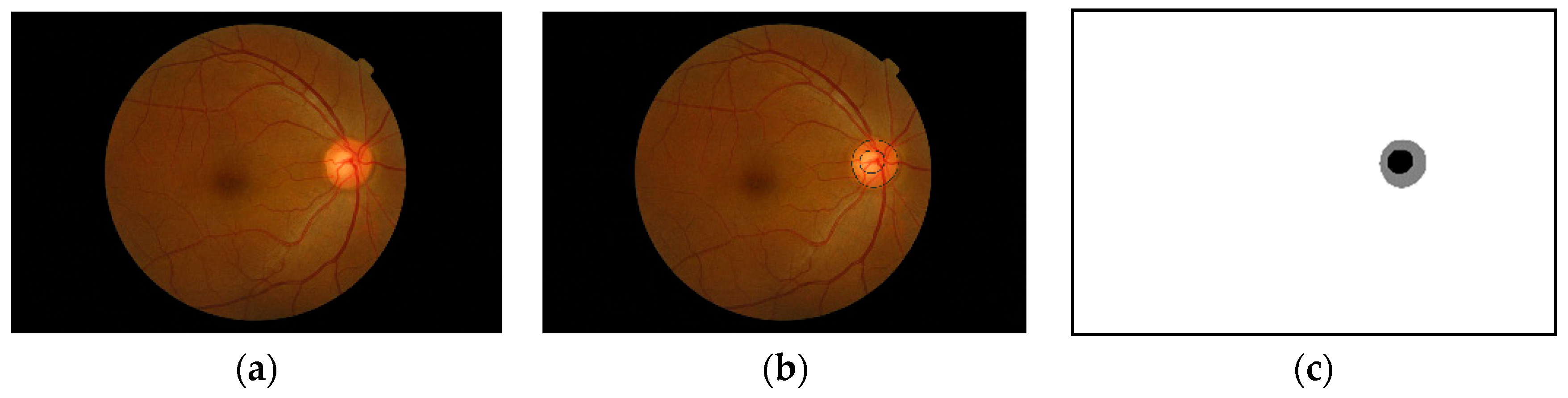Figure 1 shows an example of a fundus image and the optic nerve head along with an annotated optic disc and cup boundaries. Some standard measures used to detect the changes in the optic nerve head are the vertical cup-to-disc ratios and the cup-to-disc area ratios [5]. If we get accurate segmentation masks for the optic disc and optic cup, we can efficiently compute these ratios. As shown in Figure 1, the ONH occupies a small portion of the fundus image, and the rest of the image is considered background. Working with a tiny object within a large image does not yield a good segmentation result; also, if there are artefacts, such as high illumination, it can deteriorate the segmentation accuracy. Another problem that might arise when using the full-size image is the effect of different cameras used to capture the images. The ONH might look visually similar when using different cameras, but the background will differ a lot. Localizing the ONH within the fundus image and doing the segmentation on the cropped image around the ONH can help the segmentation process. The perimeter of the ONH is the same as the optic disc, but for localization purposes, we will refer to the ONH because localizing the optic cup which is part of the ONH is considered as localization of the ONH itself.

2. Related Work

Image segmentation is a prevalent task in computer vision applications. In recent years the advancement in deep learning algorithms and libraries led to a significant adoption of deep learning in computer vision tasks, including classification and segmentation. Prominent deep learning architectures for segmentation includes U-Net [6] and Mask R-CNN [7]. Algorithms were developed to localize and detect the optic disc with methods such as interval type-II fuzzy multi-level thresholding [8]. Another classical image processing approach was proposed by Mittapalli and Kande [9]; their approach consists of locating the optic disc using PCA, blood vessels segmentation and inpainting, optic disc segmentation using extended local binary fitting (LBF) active contour, and cup segmentation using spatially weighted fuzzy c-means (SWFCM) clustering. This approach is fascinating but very involved, unlike the deep learning end to end approach. The approach was trained and tested on 59 images only, which does not give enough information about the robustness of the approach. Mitra et al. [10] used a convolutional neural network for localization by dividing the image into 13 × 13 regions and framing the problem as regression to find the bounding box then use non-maximum suppression on the 13×13 gird prediction for the final bounding box. For segmentation, Feng et al. [11] used modified U-Net with short and long skip connections inspired by ResNet [12] to segment optic disk and exudate but not the optic cup. Edupuganti et al. [13] used a VGG16 style fully convolutional neural network (FCN) pre-trained on ImageNet to segment the optic disc and cup in Drishti-GS dataset [14]. The ONH in these images is centered in the image; hence they only center cropped the images to preserve the image resolution. Orlando et al. [15] released the REFUGE dataset along with the REFUGE challenge as an attempt to have a standardize benchmarking strategy for comparing different models for both segmentation and classification tasks. The training set has a different resolution and was acquired with a camera that is different from the validation and test sets (details on this are provided in the materials section). The competition was conducted in two phases and only 12 teams made it to the final stage, and their results were reported in the paper [15]. Each team used a different approach to tackle the segmentation problem. Most teams used a two-stage approach for segmentation which proved to be successful in many cases [16]. AIML team used a ResNet-50 based FCN to locate the ONH then crop around it to one-quarter of the original size; the cropped images are then passed to four more ResNet networks ResNet-50, -101, -151, and -38 to segment the OD/OC. They used the REFUGE training set with augmentation to train the network. Test time augmentation is used in the four networks, and the final result is averaged across all individual outputs. BUCT team used two U-Nets [6] one for OD segmentation and the other for OC segmentation. First, they cropped the image to a square of size 817 × 817 keeping the ONH in the left side of the image, as the OHN in REFUGE dataset is located at an almost fixed general area within the fundus image. The cropped image is then resized and used for OD detection by the first U-Net, and ellipse fitting on the largest connected component was considered the OD. For the OC, the bounding box of the detected OD is used to crop the image with 100 pixels padding. The cropped image is fed to the second U-Net and the largest connected component is taken as the OC. Both U-Nets used REFUGE training set with data augmentation for the training process.

CUHKMED team also used a two-stage approach, first localizing the OD using U-Net then using DeepLabv3+ [17] for segmentation. They also used patch-based output space adversarial learning [18] to tackle the difference between the training and test/validation sets. The final segmentation is computed using an ensemble of five models. They used the training set from REFUGE to train the network and the training combined with validation set for adversarial learning. Cvblab team used a two-stage U-Net, the first one to detect and segment the OD, and the result of this is used to crop the image for OC segmentation. The OC segmentation is done using another U-Net specially trained to capture OC from the cropped image. Contrast Limited Adaptive Histogram Equalization was also used as a preprocessing step. Unlike the previously mentioned approaches, Cvblab team used extra data for the training including, REFUGE training set, DRIONS-DB, DRISHTI-GS, and RIM-ONE v3.

The Mammoth team used Mask R-CNN for OD localization and segmentation then Dense U-Net for segmentation. The Mask R-CNN output is used to crop the image around the detected OD, and the cropped image is used as input to the Dense U-Net. The Dense U-Net is used to get another segmentation of the OD. They used the probability values from the first OD segmentation output as an extra input layer for another U-Net to segment the OC. The output of both networks is ensembled to get the final prediction. The Masker team also used Mask R-CNN at the first stage to localize the ONH and crop the image around it. In the second stage, the training set was divided into 14 subsets using the bagging technique. The images were preprocessed with different techniques. Each subset is trained with Mask R-CNN, U-Net, and Mnet for OD and OC segmentation and the final segmentation result is determined using voting among all the networks. NightOwl team used two dense U-Nets; the first gives a coarse localization of the ONH and then the image is cropped around the localized ONH. The other network performs the segmentation. Post and pre-processing steps were used to enhance the detection such as histogram matching and exponential transform in preprocessing as well as morphological operations and Gaussian smoothing in postprocessing. An augmented version of the REFUGE training set was used to train the network; augmentation was used to reduce the imbalance between glaucoma and non-glaucoma samples. NKSG team used DeepLabV3+ for the segmentation and used the ONH area as input to the network. They did not mention explicitly how the ONH area was selected, whether it was automatically found or manually cropped. Pixel quantization was also used as a preprocessing step. SDSAIRC team also used a cropped version of the image for the training of their multistage networks. The Mnet was used for both OD and OC segmentation. First, the predefined region of interest (ROI) of the fundus image was fed to the first Mnet to detect the OD then a bounding box around the detected OD was used to crop the image further and feed it to another Mnet for OC segmentation. The output was then post-processed using ellipse fitting. Histogram matching was used to transform the test and validation images to match the training image set.

SMILEDeepDR used a different approach where a modified U-Net with squeeze and excitation was used for both glaucoma classification and for optic cup/disc segmentation. The inclusion of squeeze and excitation approach to U-Net was introduced by Rundo L. et al. [19] for prostate zonal segmentation on Magnetic Resonance (MR) images. The SMILEDeepDR team trained the network first to carry the classification task then a new network was fine-tuned to conduct the segmentation starting with the classification network weights. The segmentation was posed as an L1 loss rather than cross-entropy. VRT team used a modified U-Net with an auxiliary CNN branch that takes the vessel segmentation mask to generate estimated OC/OD masks. The output of this network is connected to the bottleneck layer of a second U-Net to obtain the final segmentation. The training loss is calculated using the vessel segmentation loss and the final segmentation loss. The generated masks are then post-processed by filling the holes and generating convex hulls from the results. Finally, WinterFell team used Faster R-CNN first to detect and crop the ONH then a ResUnet for OD/OC segmentation. They used two preprocessing steps, first normalizing all images using a reference image then inverting the green channel from the RGB color space.

A common problem with medical image analysis is the limited amount of data which can be tackled by synthesizing new data using, for example, conditional generative adversarial networks [20], using extreme augmentation [21], or leveraging transfer learning [22]. We use the transfer learning technique in this paper. Kandel and Casteill in their review article [23] gave an overview of six convolutional neural network architectures that are usually used in transfer learning and they listed their applications in diabetic retinopathy classification in the literature.

For this paper, we used the REFUGE dataset with its train/test split setting, and we added Magrabi male, Magrabi female, and MESSIDOR datasets from [24] as additional test sets to check the robustness of the proposed solution. The ONH inside Magrabi and MESSIDOR fundus images is not located in a fixed position, like for example the center of the images (Drishti-GS), or in the center-left side of the image (REFUGE), images from Magrabi and MESSIDOR data sets have the ONH in different areas of the image. Hence, we cannot merely center crop the images or crop the image around the center-left as some teams did in the REFUGE challenge. Our approach includes first localizing the ONH from the image and cropping around it, then using the cropped portion of the image for segmentation. For both tasks, Mask R-CNN is used, and unlike most of the teams in the REFUGE competition, we will not use an ensemble of network or augmentation for segmentation.

The following are this paper’s main contributions:

• Simpler and less computationally expensive method compared to state-of-the-art for retinal fundus image segmentation. The top-performing team in the REFUGE challenge utilized data other than the training set and used an ensemble of many Mask-RCNNs. Our method with a hierarchal approach with only two Mask-RCNNs and a training trick by modifying the loss weight for the second stage in the training reached the level of the top-performing team. The model trained well with this method transfer to other datasets without being retrained.
• A new training strategy for fine-tuning a network for improved detection of optic nerve head from fundus images. This includes changing the region proposal network detection scales and using the cropped images from the first stage alongside the original images for the training.

The remainder of this paper consists of four sections: (1) Materials and Methods: contains a description of the architecture, details about the methodology, and the datasets used. (2) Results: present the experimental results of the proposed method on the datasets described in the previous section. (3) Discussion and conclusion: a short discussion about the results, final remarks, and possible future work.

3. Materials and Methods

Since our method is based on a two-stage Mask R-CNN, we first provide a brief review of this network. The Facebook AI Research group developed Mask R-CNN in 2017 [7]. It is an extension to Faster R-CNN [25], where an extra head is added to the network to perform instant segmentation, Faster R-CNN starts with a backbone for feature extraction. The backbone is followed by a region proposal network (RPN), and two head branches, one for bounding box regression. The other is for classification, the added branch in Mask R-CNN uses the region of interest (ROI) in a fully convolutional network to predict a mask for that ROI. All of the three heads utilize features extracted by the backbone network, which is usually a ResNet [12]. The ROIs are extracted using the region proposal network (RPN). The weights of the network are adjusted during the training using five loss values with a total loss calculated as follows.

$$\begin{array}{l}loss=w_1\times rpn\_class\_loss+w_2\times rpn\_bbox\_loss\\ +w_3\times class\_loss+w_4\times bbox\_loss\\ +w_5\times mask\_loss\end{array}$$

(1)

The RPN class loss and RPN bounding box loss are related to the output of the region proposal network. The RPN class loss is a binary classification loss; it is considered positive if the intersection over union (IoU) of the proposed region with a ground truth bounding box is >0.7. The RPN bounding box loss is a regression loss between the four corner points of the ground truth bounding box and the proposed region bounding box. The RPN produces multiple regions which may have a significant overlap; a non-maximum suppression algorithm is applied to these regions to discard regions with overlap and produce regions of interest. The features maps corresponding to the ROI are cropped from the backbone and aligned before using them in the three heads to produce the bounding boxes, classification, and segmentation masks.

Recall that our main problem is segmenting the optic cup and optic disc from the fundus images, then calculating the cup to disc ratio from the segmentation masks. The optic cup and optic discs are in the optic nerve head. The size of the optic nerve head is tiny compared to the fundus image, and the optic cup is even smaller; hence finding and segmenting the optic cup is hard. Using Mask R-CNN on the entire fundus image will localize the ONH well but cannot segment the optic cup adequately and sometimes fails to detect it.

3.1. Method

One advantage of Mask R-CNN is that it gives both bounding box and semantic segmentation, this allows for a multi-stage approach for semantic segmentation using the same architecture. The first stage is analyzing the image with its original view/zoom scale, and the second stage focuses on the optic nerve head and zooming into it for further analysis.

3.1.1. Stage 1 Training

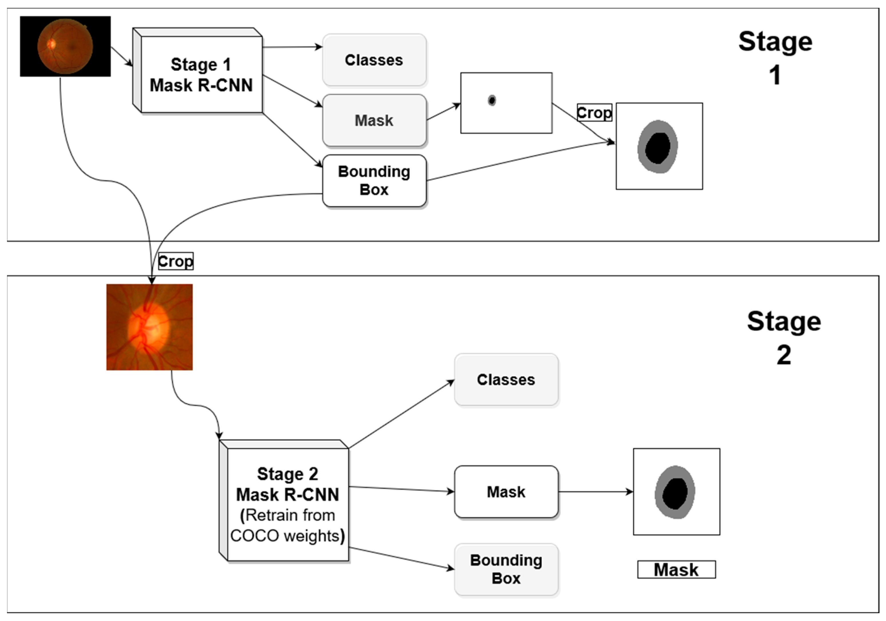
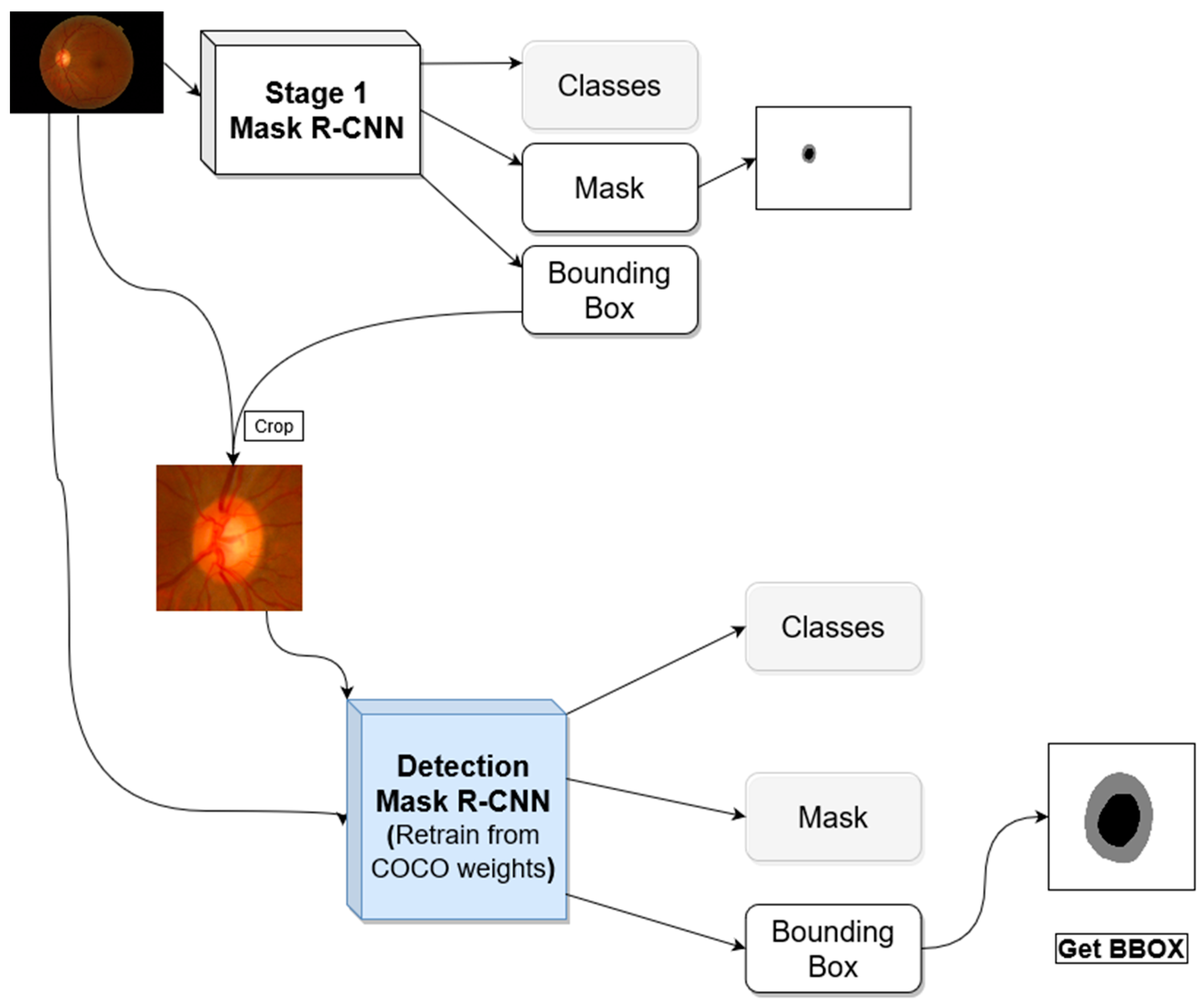
Figure 2 shows the general architecture for the proposed segmentation method. The first stage produces optic disc segmentation that is not perfect but has high dice score accuracy. The optic cup segmentation, however, is not proper, especially when using the trained model in a new dataset outside the distribution of the dataset used in the training.

In the first stage, we use a Mask R-CNN network with initial weights pre-trained on the COCO dataset. We froze the backbone weights before the C3 block and allowed the rest of the weights to become tuned during the training. C3 refers to stage 3 downsampling block (Conv3_x) of the ResNet [12]. The resulted bounding box from this stage is used to crop the image around the ONH and feed the cropped image to the second stage. The first stage network investigates the entire image to locate and segment the optic disc/cup. With images coming from different distribution due to different acquisition devices, the model will not have the same performance on the new datasets. Most of the differences in the fundus image happen in the retinal background (background with respect to the ONH).

3.1.2. Stage 2 Training

For the second stage, we hypothesized that the ONH and its parts (OD/OC) are usually visually similar across datasets, so emphasizing the mask loss during the training will help in boosting the performance, even if a dataset that is originally from a different distribution is used for testing. To test this hypothesis, we performed two experiments in the second stage. In one experiment, the weights associated with each loss in Equation (1) are set to 1, and in the second experiment, the weights of the bounding box and mask (w4, w5 in the equation) were increased to 1.5 and 2.0, respectively. The bounding box weight is increased because the masking process depends on finding a proper bounding box around an object, hence it is increased slightly to make sure a bounding box is found first before attempting to do the segmentation. The Mask R-CNN in stage 2 also used COCO pre-trained weights as starting point, and all layers before C3 are frozen during the training. After localizing the optic nerve head in stage 1, its bounding box is used to crop the image to be used for the analysis in the second stage. The bounding box is padded with extra pixels from each side before using it for cropping the image to get more context for the ONH for better analyses.

To assess the performance of the proposed method, we use different parameters; the first stage is judged with one more parameter compared to the second stage. In the first stage, we are concerned with two outcomes of the network: the localization of the optic nerve head (which includes the optic disc and optic cup) and the segmentation of the optic disc and the optic cup.

Assessing the segmentation in the first stage will help us to determine if the extra steps of cropping the images and training another model are worth the effort. In the second stage, we are not concerned much about the localization; we care more about the segmentation. The bounding box of the optic disc or the optic cup will be used to assess the accuracy of the localization in the first stage. From the experiments (especially when using a dataset with distribution outside the training dataset), we saw that sometimes the optic disc is not detected by the network. However, the optic cup is detected. Hence the optic cup detection will also be used to determine the success of localization if the optic disc is not detected correctly. The strict definition of the localization used in the literature is the intersection over union (IoU), also known as the Jaccard index or Jaccard score, which is defined in Equation (2).

$$IoU=\frac{\left|A\right|\cap \left|B\right|}{\left|A\right|\cup \left|B\right|}$$

(2)

where IoU is the Jaccard score (intersection over union), A is the ground truth bounding box (or segmentation mask), B is the predicted bounding box (or segmentation mask). The bounding box is used to assess localization accuracy while the segmentation mask is used to assess the segmentation accuracy.

Another standard measurement for medical image segmentation is the Dice score which is related to the Jaccard score by Equation (3).

$$D=\frac{2J}{1+J}$$

(3)

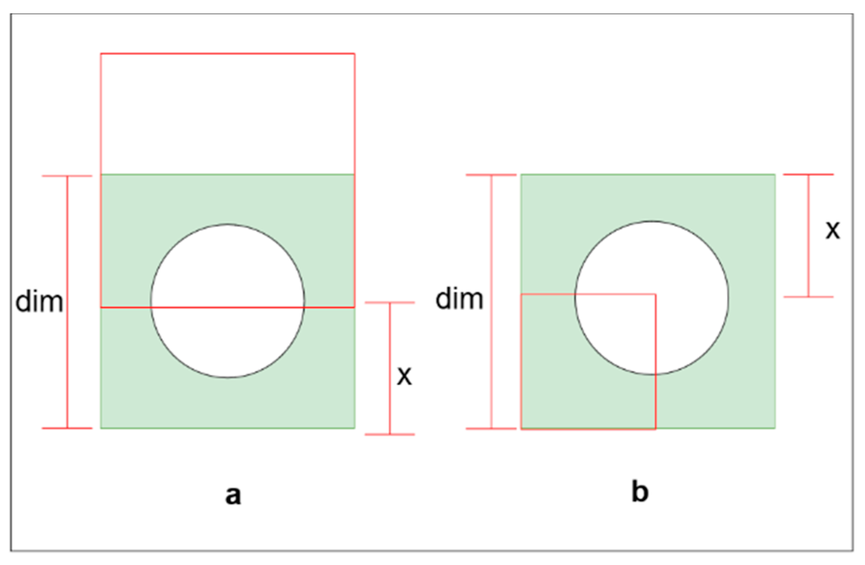
where D is the dice score, and J is the Jaccard score (IoU). We will report the results using the Dice score to have comparable results with the literature. Since we are padding the bounding box, we can use a loose definition for successful localization, still based on IoU. We need to find the minimum IoU needed to contain the entire ONH for a given padding size. There are two situations where we need more padding to cover the ONH (Figure 3). The first one (Figure 3b) is if the predicted bounding box has a portion outside the ground truth bounding box and the reset overlap the ground truth.

The second situation is when the predicted bounding box lay entirely inside the ground truth. In the second situation, for a given IoU, the maximum padding is required if the bounding boxes shared a corner (Figure 3b).

If the predicted bounding box is to move or change in size to require a larger padding, it will no longer have the same IoU. To calculate the minimum IoU required for a given padding size, we can use Equations (4) and (5).

$$Io{U}_{outside}=\frac{dim-x}{dim-x}$$

(4)

$$Io{U}_{inside}=\frac{{dim}^2-2dimx+x^2}{{dim}^2}$$

(5)

where dim is the dimension of the ONH ground truth bounding box in pixels, x is the padding size in pixels, IoU_outside is the minimum IoU for the case where a portion of the predicted box is outside the ground truth, and IoU_inside is the minimum required IoU when the predicted bounding box falls entirely inside the ground truth bounding box. The dataset contains images with varying resolutions and varying ONH diameter sizes. The largest ONH bounding box diameter across datasets is 401 pixels. 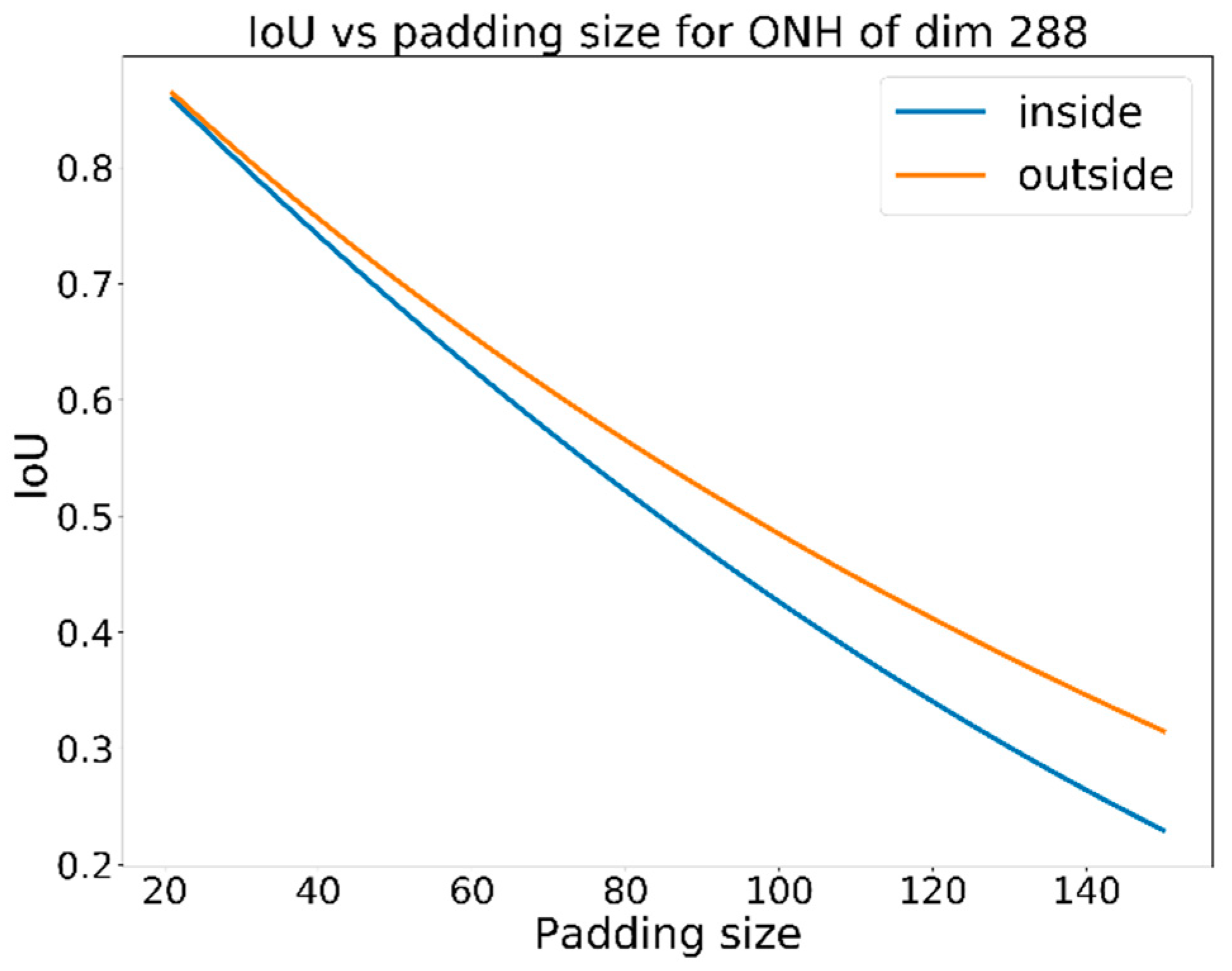Figure 4 shows the required padding vs. IoU for a fixed ground truth bounding box with a dimension of 401 pixels. For a padding size of 100 pixels, an IoU of 0.56 minimum is required, but in our calculations, we will use a larger IoU threshold of 0.60 to determine the success of localization. If the optic disc is not detected, but the optic cup is detected, the same criteria for success localization will be applied. However, when cropping the image, padding of 150 pixels will be used instead of 100 pixels.

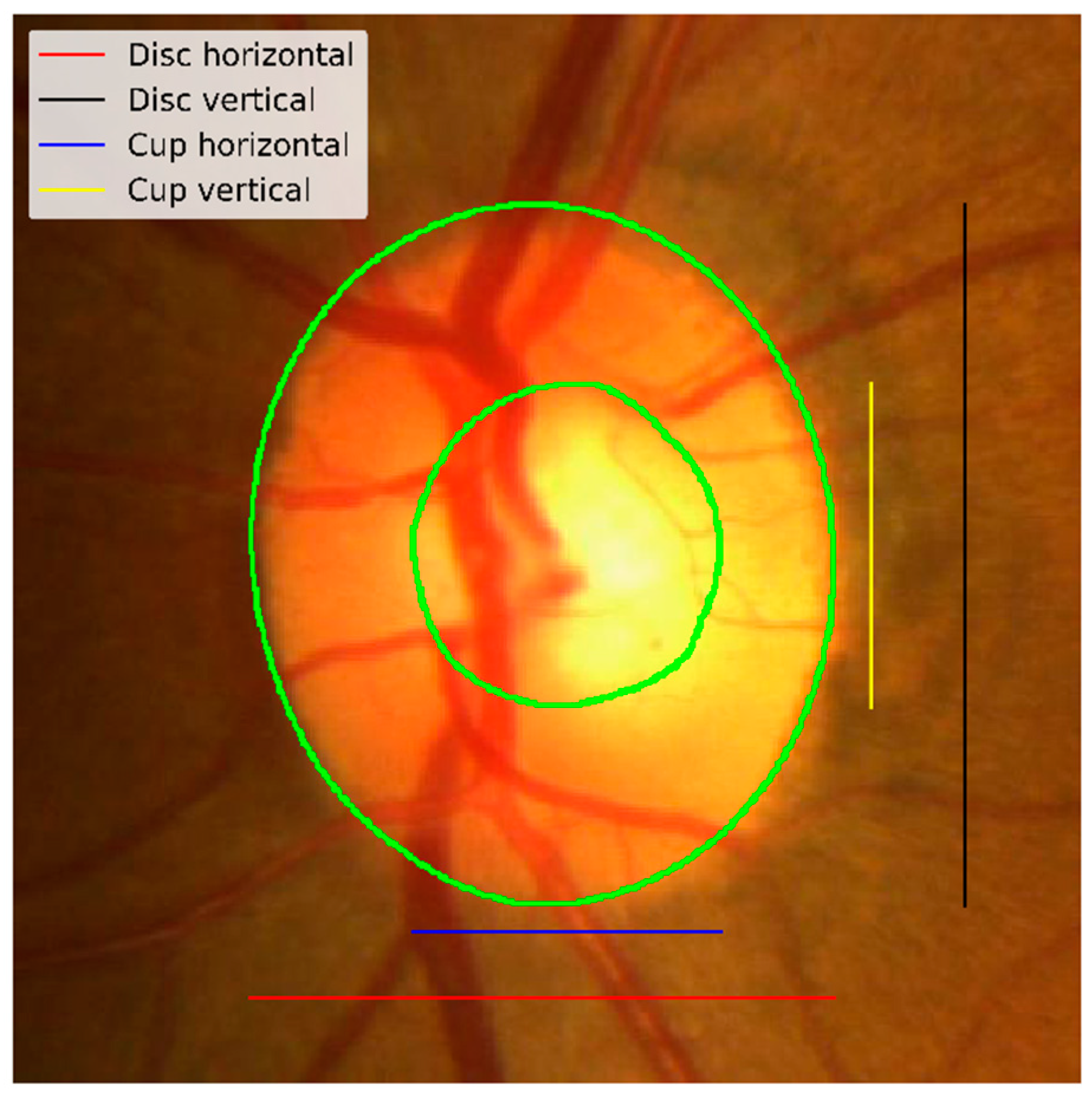
The segmentation accuracy can be measured using five values: the optic disc Dice score (Equation (3)), the optic cup dice score, the cup-to-disc area ratio (CDR), the horizontal cup-to-disc ratio (hCDR), and the vertical cup-to-disc ratio (vCDR). Figure 5 shows an example of vertical/horizontal cup and disc measurements used for hCDR and vCDR calculation. The proposed method will be assessed based on three measures: the optic disc Dice score, the optic cup Dice score, and the absolute error in the vertical cup-to-disc ratio (vCDR) to compare the approach with the reported results in the REFUGE challenge.

3.1.3. Improving Stage 1 Training

The network that we train for stage 1 (ONH detection) will face difficulties when it is used for an out of distribution dataset. Different datasets acquired by different devices will have different resolutions and different visual characteristics; the location and the size of the ONH will be different. When resizing the fundus images to a fixed size for training or inference, the entire retina might be mistaken for the optic disc. We are proposing a new method for training the localization network, as depicted in Figure 6. The proposed training method consists of two stages; the first stage is training a Mask R-CNN on the original image and uses the resultant bounding boxes to crop the training images and their ground truth annotations. The second stage uses a mix of the original and cropped images for training. To accommodate the different sizes of the ONH, the detection network in the second stage utilizes smaller RPN anchor scales [26], and the images are resized to 512 × 512 instead of 1024 × 1024.

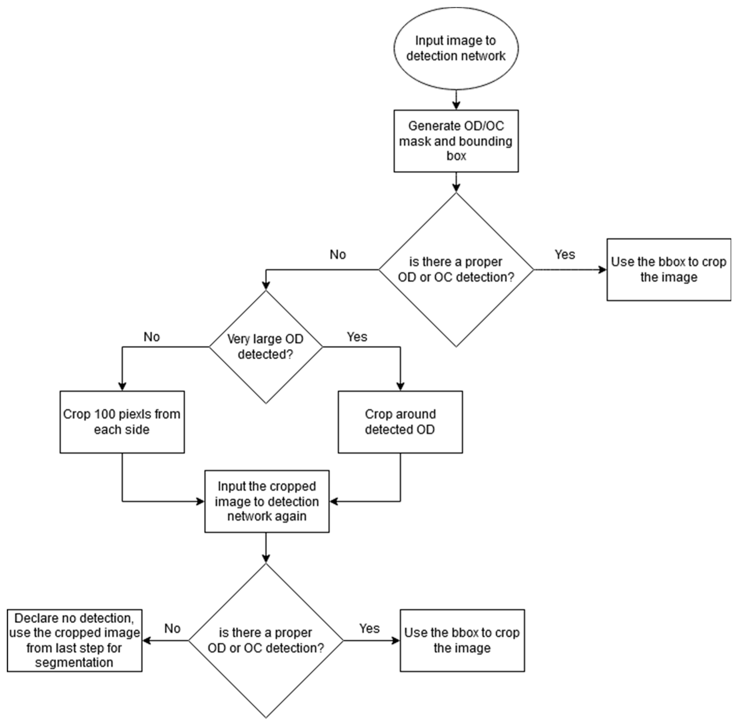
After training the network, the detection network is used following the flow chart in Figure 7. The fundus image is first put through the detection network; if OD or OC is detected, its bounding box is used to localize the ONH and crop the image. If no OD or OC is detected it either means nothing is detected or the whole retinal area is detected as OD (the area of the detected OD is very large compared to the original image size). If nothing is detected, the input image is cropped by 100 pixels in each side and passed again to the detection network. If large OD is detected, the image is cropped around the detected area and passed again to the detection network.

3.2. Datasets and the Mask R-CNN Implementation

Mask R-CNN implementation by Matterport [27] was used to conduct the experiments. The code is implemented using TensorFlow framework (version 1.4) from Google and it was run on an HP OMEN 900-251nx with NVIDIA GeoForce GTX 1080 graphics card. The original implementation of Mask R-CNN used a fixed learning rate of 0.02 that was decreased to 0.002 toward the end of the training; a weight decay of 0.0001 was also used. In Matterport’s implementation, the default learning rate is set to 0.001 with a comment about weights explosion that might be due to optimizer differences. The original paper used a step decrease learning rate with a single step, and the TensorFlow implementation by Matterport did not use any. We noticed that using weight decay only did not help to combat the overfitting problem in our case; hence a learning rate decay was added. The REFUGE training dataset was used to train the networks. The proposed method performance is tested on the REFUGE validation set, REFUGE test set, MISSEDOR, Magrabi Male, and Magrabi Female datasets.

Table 1. Datasets used in training and testing.

Data Set	Number of Images	Acquisition Device	Resolution
REFUGE training	400	Zeiss Visucam 500	2124 × 2056
REFUGE validation	400	Canon CR-2	1634 × 1634
REFUGE testing	400	Canon CR-2	1634 × 1634
MISSEDOR	460	Topcon TRC NW6	2240 × 1488, 1440 × 960
Magrabi Male	47	Topcon TRC 50DX	2743 × 1936
Magrabi Female	47	Topcon TRC 50DX	2743 × 1936

lists the information about the training and testing datasets used in the experiments.

As you can see from Table 1, the datasets were acquired using different cameras and have different resolutions. Magrabi and MESSIDOR dataset contained six ground truth annotations by six different ophthalmologists; the ground truth for these subsets was computed using the average ground truth from the six ophthalmologists.

4. Results

The segmentation task is composed of two stages; the first stage is localizing the ONH and cropping the image and the second stage is the segmentation on the cropped image. Both stages produce bounding boxes and segmentation masks.

4.1. Segmentation Stage 1

In this stage, the original images are used for training and testing, and only one experiment was performed. The output of this stage is a bounding box and segmentation masks for the optic disc and optic cup.

Experiment # 1:

In this experiment, the images were resized to 1024 × 1024 after being padded with 0 to maintain the aspect ratio of the original image. The backbone network used the weights pre-trained on the COCO dataset. The backbone’s first few layers (from input until C3) were frozen during the training; the weights of the rest of the network were updated using the total loss defined in Equation (1), with all weights being equal.

The bounding box output was used to crop the original image and the ground truth masks to be used in stage 2 training and testing. Each bounding box was padded with 100 pixels on each side. The network used resnet101 as a backbone, and the training ran for 500 epochs with an initial learning rate of 0.001, a learning rate decay of 0.0001, and a weight decay of 0.0001. We trained the network using the REFUGE training dataset.

4.2. Segmentation Stage 2

In this stage, the cropped images from stage 1 are used as input to the second Mask R-CNN network. The ground truth is also cropped based on the same bounding box from stage 1 output.

Experiment # 2: Using the same loss weights

This experiment used the same weight (Wx = 1) for the total loss calculation in Equation (1). The cropped images were resized to 512 × 512. The training was run for 500 epochs with an initial learning rate of 0.001, a learning rate decay of 0.0001, and a weight decay of 0.0001. The network was initialized using the weights from a network pre-trained in the COCO dataset. Like stage 1, the first few layers (input to C3 in the backbone) were frozen, and the rest of the network weights were updated during the training.

Experiment # 3: Using different loss weights

This experiment used the same configuration and parameters of experiment 2 except for the weights of different losses in Equation (1). This experiment examined the effect of using different loss-weight for different loss components. Since we emphasized the segmentation rather than localization in this stage, the mask loss weight (W5 in Equation (1)) was set to 2.0, and the bounding box loss (W4) was set to 1.5, and the remaining weights were set to 1.0 (default value).

4.3. Localizaion Network

The new localization network is a Mask R-CNN network that uses the cropped images from stage 1 as well as the original images in the REFUGE training set to train a more sophisticated localization network. Here both original and cropped images are resized to 512 × 512 with 0 padding to preserve the aspect ratio. We use the same network architecture that is used in stages 1, and 2 with the following modification: (1) replace the RPN anchor scales 128 and 512 with 8 and 16 to accommodate for different ONH sizes from original and cropped images. (2) The mask loss weight (W5 in Equation (1)) and the bounding box loss (W4) are set to 2.0, but the remaining weights are set to 1.0. (Equation (3)). All the layers of the network are updated during the training, not just layers below C3 in the backbone.

Table 2. Segmentation accuracy results.

		Stage 1	Stage 2
Dataset	Measure	Exp1	Exp2	Exp3
REFUGE Training	Disc Dice	0.9802	0.9634	0.9705
	Cup Dice	0.9776	0.9237	0.9358
	vCDR error	0.0137	0.0281	0.0263
REFUGE Validation	Disc Dice	0.9425	0.9489	0.9426
	Cup Dice	0.8225	0.8643	0.8531
	vCDR error	0.0815	0.0466	0.0410
REFUGE Test	Disc Dice	0.9504	0.9477	0.9334
	Cup Dice	0.7883	0.8546	0.8302
	vCDR error	0.0979	0.0425	0.0430
MESSIDOR	Disc Dice	0.9001	0.8852	0.8133
	Cup Dice	0.4174	0.7069	0.7195
	vCDR error	0.2819	0.0955	0.0785
Mag. Male	Disc Dice	0.9516	0.9237	0.9139
	Cup Dice	0.7098	0.7373	0.8190
	vCDR error	0.1391	0.0960	0.0685
Mag. Female	Disc Dice	0.8985	0.8695	0.8733
	Cup Dice	0.6673	0.8009	0.8411
	vCDR error	0.1634	0.1042	0.0855

shows the results of the segmentation average accuracy for disc/cup Dice scores and vertical cup-to-disc ratio. Except for the REFUGE validation set, the disc Dice score is higher in stage 1 when the whole image is used for segmentation. This could be due to a broader context for segmentation and the fact that the optic disc is visually different from the background in most of the images, and it is easier to identify from the whole image. We can see from the table also that using the cropped images yielded a better cup Dice scores. Experiment 2, where the loss weights are equal, gave better results in REFUGE validation and test set but did not generalize to the other three datasets, namely MESSIDOR, Magrabi Male, and Magrabi Female. When it comes to the most crucial part for the diagnosis, i.e., vCDR, you can see that experiment 3, where we have different weights for the loss function, yielded the best result across the datasets.

Table 3. Localization network accuracy results.

Dataset	Measure	Stage 1 Network	Proposed Localization Network
REFUGE Training	ONH detection	1.0000	1.0000
REFUGE Validation	ONH detection	0.9950	0.9975
REFUGE Test	ONH detection	0.9975	1.0000
MESSIDOR	ONH detection	0.9522	0.9804
Mag. Male	ONH detection	1.0000	1.0000
Mag. Female	ONH detection	0.9149	1.0000

shows the localization accuracy using the network from stage 1 and the proposed new localization network. The ONH is considered detected according to the criteria discussed in the materials and methods section if the IoU > 0.6, for either the optic disc or optic cup. If both optic disc and optic cup are detected, the optic disc bounding box is used to do the cropping. As shown by the data, the proposed localization network performed better across the datasets. As far as we know, there is no benchmark training on REFUGE and testing on Magrabi and MESSIDOR datasets for segmentation; hence the comparison will be made with the top three performers on the REFUGE challenge [15] on the REFUGE test dataset for the segmentation purpose. For the localization, we will compare it with the localizing method used in [24], which has localization scores for Magrabi and MESSIDOR datasets.

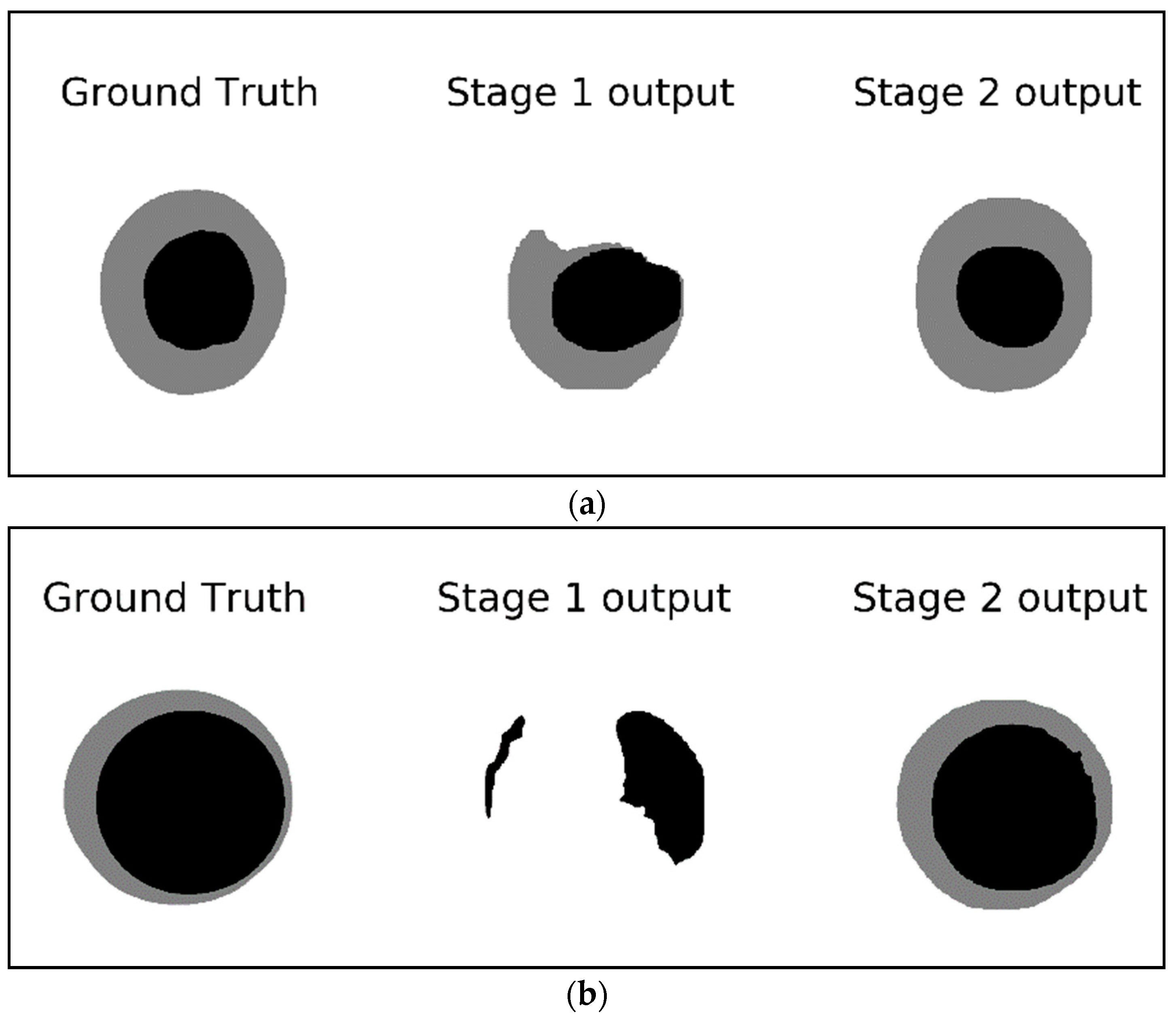
Figure 8 shows examples of the detected masks in stage 1 and stage 2 compared to the ground truth mask. Figure 8a demonstrates how the output of the second stage is closer to the ground truth while the output of the first stage looks deformed and is missing a big chunk of the optic disc. Figure 8b shows an example of missing the entire optic cup and most of the optic disc in the output of the first stage network whereas the second stage output provides a good segmentation result for both the optic cup and the optic disc. These examples signify the improvements gained by using a two-stage network compared to a single Mask-RCNN. The single stage network (stage 1 network) is looking at a small part of the image representing the region of interest for the segmentation; such a tiny RIO is difficult to analyze especially if the original image is resized to a smaller dimension to preserve the computational resources. The second stage, however, is looking at the ROI itself ignoring all the background seen in stage 1. This allows for more features to be extracted from the ROI rather than the background which help in producing more accurate segmentation.

As you can see from

Table 4. Comparing segmentation accuracy.

Method	Optic Cup	Optic Disc	vCDR
Team CUHKMED [15]	0.8826	0.9602	0.0450
Team Masker [15]	0.8837	0.9464	0.0414
Team BUCT [15]	0.8728	0.9525	0.0456
Proposed method (same loss weight)	0.8546	0.9477	0.0425
Proposed method (different loss weight)	0.7182	0.9334	0.0430

, the accuracy of the vCDR, which is used for diagnosis, is approaching the state-of-the-art level with 0.0016 mean absolute error difference. This result is achieved without using an external dataset, augmentation, preprocess, postprocessing, or ensemble method. The best vCDR accuracy in the REFUGE challenge was achieved by team Masker by applying different preprocessing techniques and using an ensemble with three types of networks trained on 14 subset partitions using bagging, totaling 42 networks, which is computationally expensive.

Table 5. Comparing the localization accuracy.

Dataset	Proposed Localization Network	Interval Type-II Fuzzy Entropy Based Thresholding [24]
MESSIDOR	0.9804	0.967
Magrabi	1.0000	0.936

shows that the proposed localization network outperformed what has been reported previously on MESSIDOR and Magrabi.

5. Discussion and Conclusions

In this paper, we proposed a method of localizing the optic nerve head and segmenting the optic disc and optic cup, which are used to calculate the vertical cup to disc ratio for glaucoma diagnosis. The method is based on a two-stage Mask R-CNN. The localization network is trained using the original and cropped fundus images and tested on the task of localizing the ONH in the full image, which gives detection accuracy between 98.04% and 100% on the test datasets which came from different acquisition devices and have different resolutions. The segmentation Mask R-CNN network is trained using different weights for the loss function components which help in improving the performance of the segmentation on different datasets from different acquisition devices and having different distributions. The network was trained in the REFUGE training dataset and tested on REFUGE validation/test sets as well as MESSIDOR and Magrabi. The proposed method achieved a state-of-the-art performance without the computational complexity used to get the state-of-the-art results in the REFUGE challenge. The top-performing team (Masker team) at the REFUGE challenge in terms of vCDR (which is used for the diagnosis) used ORIGA dataset as well as REFUGE training set to train their networks. They first used one Mask-RCNN network for the initial localization. After localization, they used bagging to create 14 subsets, each trained using Mask-RCNN, U-Net, and Mnet [28]. They did not provide details on whether they modified the architecture of these networks, or they used the original architecture. Mask-RCNN backbone can be ResNet50 with 44,668,324 parameters or ResNet101 with 63,738,788 parameters. Since the backbone used is not clear from the description in the paper, we will do the calculation based on the backbone with the least number of parameters, i.e., ResNet50. The original U-Net network has 31,031,685 parameters but with modifications to the network, this number can increase. With few details on their implementation, we will calculate based on the vanilla U-Net, which usually has a smaller number of parameters compared to a modified one. The Mnet network has 8,547,720 parameters. The whole solution by the Masker team consists of 44,668,324 + 14 × (44,668,324 + 31,031,685 + 8,547,720) = 1,224,136,530 parameters in total. That is one Mask-RCNN for localization and 42 networks of Mask-RCNN, U-Net, and Mnet combined (14 of each network). Our solution consists of two Mask-RCNN networks with ResNet101 backbone with a total of 2 × 63,738,788 = 127,477,576 parameters which is far less than the 1,224,136,530 parameters in team Masker’s solution.

The optic cup/disc segmentation and vCDR calculation based on the solution provided in this paper can be used to triage patients to get proper treatment by ophthalmology specialists, especially in places where specialists are scarce. Such systems can be deployed in eye exam centers which most often have technicians but not specialists. For future work, many interesting ideas can be explored such as removing (inpainting) the blood vessels before the training and doing heavy color transformation augmentation to improve the robustness of the solution in all the test datasets.