Article

An LSTM-Based Method Considering History and Real-Time Data for Passenger Flow Prediction

School of Traffic and Transportation, Beijing Jiaotong University, Beijing 100044, China
*
Authors to whom correspondence should be addressed.
Appl. Sci. 2020, 10(11), 3788; https://doi.org/10.3390/app10113788
Submission received: 10 May 2020 / Revised: 27 May 2020 / Accepted: 28 May 2020 / Published: 29 May 2020

Abstract

:
With the development of big data and deep learning, bus passenger flow prediction considering real-time data becomes possible. Real-time traffic flow prediction helps to grasp real-time passenger flow dynamics, provide early warning for a sudden passenger flow and data support for real-time bus plan changes, and improve the stability of urban transportation systems. To solve the problem of passenger flow prediction considering real-time data, this paper proposes a novel passenger flow prediction network model based on long short-term memory (LSTM) networks. The model includes four parts: feature extraction based on Xgboost model, information coding based on historical data, information coding based on real-time data, and decoding based on a multi-layer neural network. In the feature extraction part, the data dimension is increased by fusing bus data and points of interest to improve the number of parameters and model accuracy. In the historical information coding part, we use the date as the index in the LSTM structure to encode historical data and provide relevant information for prediction; in the real-time data coding part, the daily half-hour time interval is used as the index to encode real-time data and provide real-time prediction information; in the decoding part, the passenger flow data for the next two 30 min interval outputs by decoding all the information. To our best knowledge, it is the first time to real-time information has been taken into consideration in passenger flow prediction based on LSTM. The proposed model can achieve better accuracy compared to the LSTM and other baseline methods.

1. Introduction

Public transport (also known as public transportation, public transit, or mass transit) is a system of transport for passengers by group travel systems, typically managed on a schedule, operated on established routes, and that charge a posted fee for each trip. The bus operation system is a major component of public transport and plays an important role. Ways to predict the passenger demand by bus are always the research focuses of scholars. The real-time passenger flow forecasting (observing the passenger flow in a short period time and predicting the passenger number for a next period of time) is also a very important part of the bus operation system. To solve the problem of passenger flow prediction, especially for real-time passenger flow prediction, this paper proposes a passenger flow prediction model based on the history and real-time data (HRPFP).
The HRPFP model mainly contains four parts: the feature extraction part, the history information encoding part, the real-time information encoding part, and the decoding part. In the feature extraction part, we use the Xgboost algorithm to combine the smart card data and the points of interest together. A POI is a specific point location that someone may find useful or interesting. We use the Amap application program interface to obtain the amount of different POIs around a certain bus station. The smart card data and the points of interest can be fused by a radius. We use the Xgboost algorithm to obtain the value of radius because the speed of the Xgboost algorithm is fast. In the history information encoding part, we use the long short-term memory (LSTM) structure to encode the history smart card data collected by AFCs. We arrange the history data with the index of the date to form a time series sequence. The length of the sequence is 7, which means that we use the passenger flow data of a certain period in the previous seven days to predict the passenger number in the same period for a certain day. In the real-time information encoding part, we also use the LSTM structure to encode the real-time smart card data collected by sensors. The index of the real-time data sequence is the time section, and the length of this sequence is 4, which means that we use the passenger flow data of the previous four time periods to predict the passenger number of the next two time periods for a certain day. In the decoding part, we use a four-layer neural network to calculate the passenger number in the next two time periods. Because the output is a single value, we choose a multi-layer neural network instead of the LSTM to speed up our training. Through comparative experiments, the HRPFP model can achieve better accuracy than the existing LSTM neural network and other baseline methods.
The structure of this paper is as follows. Section 1 is a brief introduction of our research purpose and the structure of the HRPFP model. Section 2 is the latest research methods in this area. Section 3 describes the HRPFP model framework and its sub-models. Results of the experiments are provided in Section 4. Conclusions are shown in Section 5.

2. Related Work

In this part, we will mainly introduce three methods used as baselines in our experiment. We will also introduce the achievements researchers made and the shortcomings of these methods. This part also gives the reason why we increase the data dimensions through POI data and use two encoder structures in our model based on LSTM. In recent years, machine learning and deep learning methods have been used in passenger flow prediction. A major method is the time series and Kalman filtering. This method treats the passenger flow on different dates as sequences or signals, and then looks for the regularity behind data by processing sequences or signals. M. Milinkovic et al. [1] used seasonal autoregressive integrated moving average (SARIMA) model to predict railway passenger flow. R. Gummadi et al. [2] chose a time series model to forecast the passenger flow for a certain transit bus station. M. Ni et al. [3] proposed a linear regression and SARIMA model to predict subway passenger flow. C. Li et al. [4] proposed a spatial–temporal correlation prediction model of passenger flow based on non-linear regression and time series data. S. V. Kumar et al. [5] used Kalman filtering to predict the traffic flow. P. Jiao et al. [6] used three revised Kalman filtering models to predict short-term rail transit passenger flow. This method has simple dimensions and high model training efficiency. However, this model may not perform very well in some cases because fewer feature dimensions are considered. In the multi-station passenger flow forecasting for a certain line, this method needs to train a model for each station, which will be very complicated.
Another major method is the support vector machine (SVM). This method can map low-dimensional data to high-dimensional space through the kernel function, and transform non-linear problems into linear problems, so it can effectively consider the influence of multiple factors on a model. M. Tang et al. [7] used linear regression and a wavelet support vector approach to forecast the passenger flow. Y. Sun [8] et al. used wavelet-SVM short-time to predict subway passenger flow in Beijing. R. Liu et al. [9] used wavelet transform and kernel extreme method to predict short-term passenger flow. C. Li et al. [10] chose clustering-based support vector regression to forecast bus passenger flow. They all achieved a lot of good results in passenger flow prediction using the SVM. However, due to the existence of outliers, this method has a large error in some cases.
Neural networks and deep learning are also applied to passenger flow prediction. In a famous machine learning paper, M. Spyros et al. [11] compared different methods in prediction based on stock market data. From his article, we can see that when the data dimension was small, the prediction accuracy of LSTM was the best. LSTM performed better than other basic machine learning methods. J. Guo et al. [12] proposed a combination method using the support vector regression (SVR) and LSTM neural network to predict the abnormal passenger flow. F. Toqué et al. [13] used LSTM neural networks to predict travel demand based on smart card data and proved the effectiveness of the forecasting approaches. S. Sunardi et al. [14] presented a useful way of observing the domestic passenger travel series using LSTM. Y. Liu et al. [15] built a deep learning architecture to make metro passenger flow prediction. H. Zhao et al. [16] tried to obtain the passenger numbers for a certain bus line using LSTM considering the weather information in Guangzhou city to improve the performance of prediction. However, in other cities like Beijing, weather information changes little. Therefore, weather information is not a good feature for all the big cities. Y. Han et al. [17] compared different LSTM gradient calculation methods in passenger number prediction, so we choose the Adam algorithm in our paper, based on Yong Han’s research. J. Zhang et al. [18] described the importance of real-time passenger flow prediction and used a linear method to predict the real-time bus passenger number. K. Pasini et al. and M. Farahani et al. [19,20] used encoder structures based on LSTM to predict passenger number and draw a conclusion that an encoder structure can improve the accuracy. That is the main reason that we use two encoder structures in our model.
To our knowledge, deep learning performs well in image recognition and natural language processing with thousands of feature dimensions. For the passenger flow forecast, the smart card data usually has a large scale, but the dimensions of the smart card data are usually less than 10. Therefore, in our opinion, increasing the dimensions of bus smart card data as much as possible is very important in improving prediction accuracy. A passenger prediction model can learn the passenger number regularity and predict the passenger number for the next few days based on the history data. Besides, a passenger prediction model also needs to predict the passenger number for the next few time periods based on the real-time data. The function of real-time passenger number prediction is an important part in providing early warning for a sudden large passenger flow rush. This is the major motivation for this paper.

3. Materials and Methods

3.1. Basic Methods

We choose the Xgboost algorithm [21] to train the best model for each bus line. Xgboost is a boosting tree model, which means this method tries to form several tree models for prediction. The sum of the predicted values of each tree is the predicted value of the sample. The function can be expressed as [21]:
y ¯ = ϕ x i = t = 1 T f t x i
where f t is the tth tree for prediction.
The Xgboost algorithm uses the following methods to form the tth tree. The loss function at the tth iteration can be expressed as:
L t = i = 1 n l y i , y i t 1 + f t x i + Ω f t
where x i represents sample of data, y i is the true value of x i , y i t 1 is the predicted value of the (t−1)th iteration, and f t x i is the model at the tth iteration. The second term Ω f t penalizes the complexity of the model.
Second-order approximation can be used to quickly optimize the objective in the general setting.
L t i = 1 n [ l ( y i , y ¯ i t 1 ) + g i f t x i + 1 2 h i f t 2 x i ] + Ω f t
where
g i = l ( y i , y ¯ i t 1 ) y ¯ i t 1 ,   h i = 2 l ( y i , y ¯ i t 1 ) y ¯ i t 1 .
We can remove the constant terms to obtain the following simplified objective at step t.
L t = i = 1 n [ g i f t x i + 1 2 h i f t 2 x i ] + Ω f t
Defining I j = { i | x i j } as the instance set of leaf j, we can rewrite Equation (4) by expanding Ω f t as follows:
L t = i = 1 n g i f t x i + 1 2 h i f t 2 x i + γ T + 1 2 λ j = 1 T w j 2 = j = 1 T [ ( i I j g i ) w j + 1 2 ( i I j h i + λ ) w j 2 ] + γ T
For a fixed structure q x , we can compute the optimal weight w j * of leaf j by w j * = G i H i + λ . Then,
L t = 1 2 j = 1 T G i H i + λ + γ T
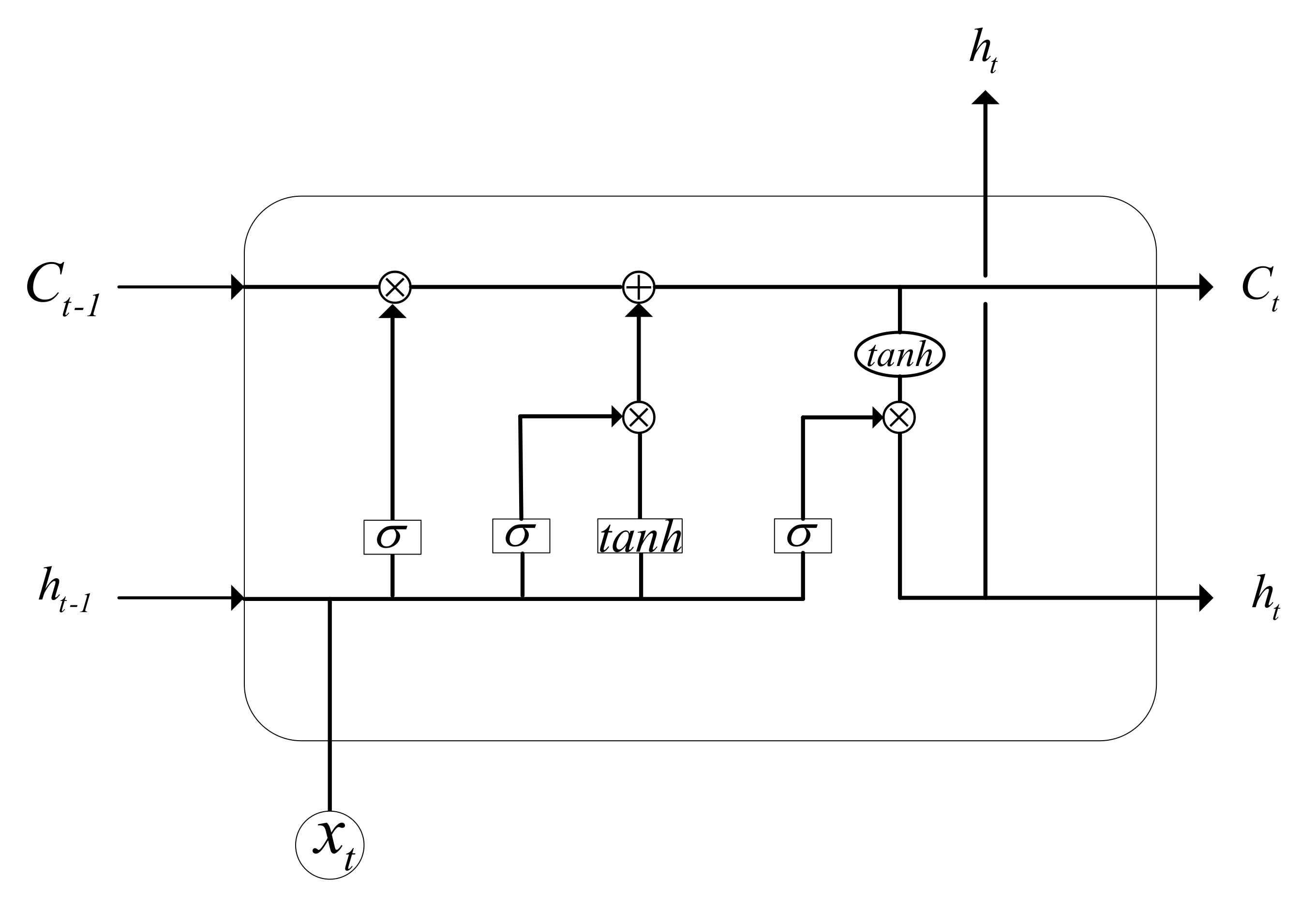
The LSTM [22] is an artificial recurrent neural network (RNN) architecture used in the field of deep learning. Unlike standard feed forward neural networks, the LSTM has a feedback connection. It can not only process a single data point (such as images), but also entire sequences of data (such as speech and video). A common LSTM unit is composed of a cell, an input gate, an output gate, and a forget gate. The cell remembers the values over arbitrary time intervals, and the three gates regulate the flow of the information into and out of the cell. The basic structure of a signal LSTM cell is shown in Figure 1.
The compact forms of the equations for the forward pass of an LSTM unit with a forget gate are:
i t = σ W ix x t + W ih h t 1 + b i
f t = σ W fx x t + W fh h t 1 + b f
o t = σ W ox x t + W oh h t 1 + b o
C t ˜ = tanh W Cx x t + W Ch h t 1 + b C
C t = i t C t ˜ + f t C t 1
h t = o t tanh C t
where t stands for tth timestamp. i t refers to the output of the input gate. f t refers to the output of forget gate, and o t is the output of output gate. x t is the input vector. C t is the state vector, and h t is the hidden vector. h t 1 is the former output of h t , and C t is the input state and output state of memory cell. σ and tanh are activation functions between different layers. is the Hadamard product. Other variables like W ix , W ih , b i are needed to be solved by minimizing the loss function.

3.2. HRPFP Model

3.2.1. The Process of HRPFP Model

This paper proposes the HRPFP model to predict the passenger number for each station at a certain line using the history data and the real-time collected passenger number. Taking one bus station as example, we obtain the history passenger data collected a few days ago, and combine these data with the point of interest (POI) data based on Xgboost to form a new dataset which contains more information. Then, we feed these data into a history data encoding neural network based on the LSTM to produce a vector that contains the history passenger information. Next, we obtain the passenger number of the previous four time periods from automatic fare collections (AFCs) and feed these data into the real-time data encoding neural network to form a vector that contains the real-time information. Then, we use a simple neural network to make the history vector and the real-time vector having the same shape. After that, we add these two vectors and produce an information vector containing both history and real-time information. Then, we encode the information vector using a multi-layer neural network to obtain the predicted passenger number for the next two time periods. The detailed process of the HRPFP model is shown in Figure 2.
In Figure 2, we can see that the HRPFP model has larger data dimensions than other LSTM passenger number prediction models. Besides, the HRPFP model also has an input containing real-time collected information. Larger data dimensions and real-time collected information can help to improve the predicted accuracy. That is why the HRPFP model had a better performance than other models theoretically.
From Figure 2, we can also obtain the forward propagation formula of the model. Let us assume that the final output of the history data encoding structure is S hx , and the output of the real-time data encoding structure is S rx . We use a linear mapping for both S hx and S rx to ensure these two vectors have the same shape. This is the major function for weights W hx and W rx . The Equations (12) and (13) show these projections.
Q h = W hx S hx + b hx
Q r = W rx S rx + b rx
To reduce the deviation caused by a too large value, we use a SoftMax function to project every element in both Q h and Q r into [0,1].
I h = S ( W hx S hx + b hx )
I r = S ( W rx S rx + b rx )
where S is the SoftMax function. Then, we use I h and I r to form an information vector, that is I v = I h + I r . After this, we use a three-layer neural network to decode the information vector I v and obtain the predicted passenger number for a period. Because the length of the output sequence is small, we use this decoding structure instead of the LSTM structure to improve the model speed. The decoding network can be expressed as:
D 1 = W d 1 I v + b d 1
D 2 = σ ( W d 2 D 1 + b d 2 )
P = W d 3 D 2 + b d 3
where σ is the Sigmoid function.
The loss function of this model is the square error between real values and predicted values, so the target is min P V 2 , where P is the predicted values and V is the real values.

3.2.2. Dataset and Data Fusion

The smart card data used in this paper come from Beijing, which is one of the largest cities in the world. In total, 6 million records are collected by AFCs every day in this city. The total dataset contains around 150 million transactions over 7000 bus stops from October 1, 2015 to October 30, 2015. All the fields we extracted from this dataset are as follows:
  • CARDID: the unique smart card ID for each passenger;
  • TRADETIME: the time that passengers got on the bus;
  • MARKTIME: the time that passengers got off the bus;
  • LINEID: the bus line that passengers took;
  • TRADESTATION: the station that passengers got on;
  • MARKSTATION: the station that passengers got off.
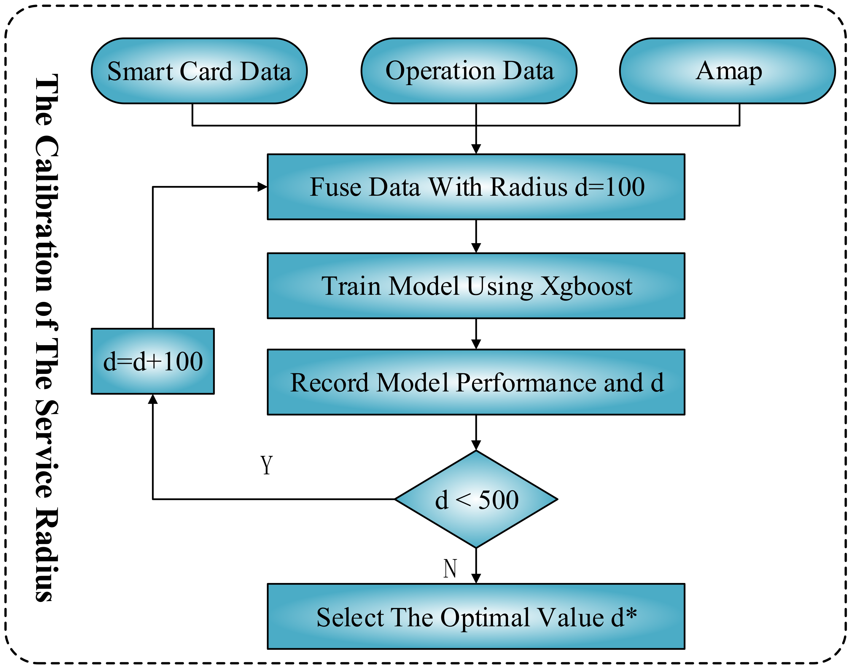
We divide the operation hours of a bus line into periods of 30 min and calculate the passenger flow in different periods based on the TRADESTATION field like Jun Zhang did [18]. The bus station information can be obtained from the bus company. The major fields used in this paper are line ID, station index, station longitude, and station latitude. We use the Amap application program interface to obtain the amount of different POIs around a certain bus station based on the distance between them. Therefore, we need an algorithm to determine the best distance. Considering a dataset D S as a sample space, a machine learning model can be expressed as M x D S y . M is a map from data point x to its real value y . When we take POIs into consideration, a new dataset will be added to the original dataset. The new model can be expressed as D n = f dis D S , D P . In this formula, D n is the new sample space, D P is the dataset of POI data, and f dis is a function based on the distance between bus stations and POIs. We change the distance from 100 to 500 m to form 5 datasets. Then, we train a machine learning model for different datasets to calculate the best service radius d* between bus stations and POI data. At last, with the help of d*, we get the most suitable dataset. The process of finding the best service radius d* is shown in Figure 3.

3.2.3. Inputs and Outputs for Encoding and Decoding Parts

There are 17 major categories of POIs, such as famous scenery, business company, shopping service and so on. After data fusing, we can extract the features feeding into two encoding parts in the HRPFP model. The date is a unique index for history data encoding. The day of the week and time section obtained from the TRADETIME field are 2 features of the time dimension. The station index, the longitude and the latitude obtained from bus operation data are 3 features in the space dimension. The different amounts of different POIs types are the other 17 features in the space dimension. Therefore, a total of 22 features are inputted to the history data encoding part. All these features should be normalized (Min–Max Normalization) before feeding into the LSTM structure. The output of the history data encoding part is a 1 × 50 vector containing a lot of information. In the real-time data encoding part, the basic information of a certain station is already considered in the history data encoding part, so we just take the real-time passenger number as the input. The input becomes a vector through the LSTM structure, then we use Equations (14) and (15) to reshape these two output vectors. Finally, we add them together to form a vector containing the history and the real-time information. The input and output of the encoding parts are shown in Figure 4.
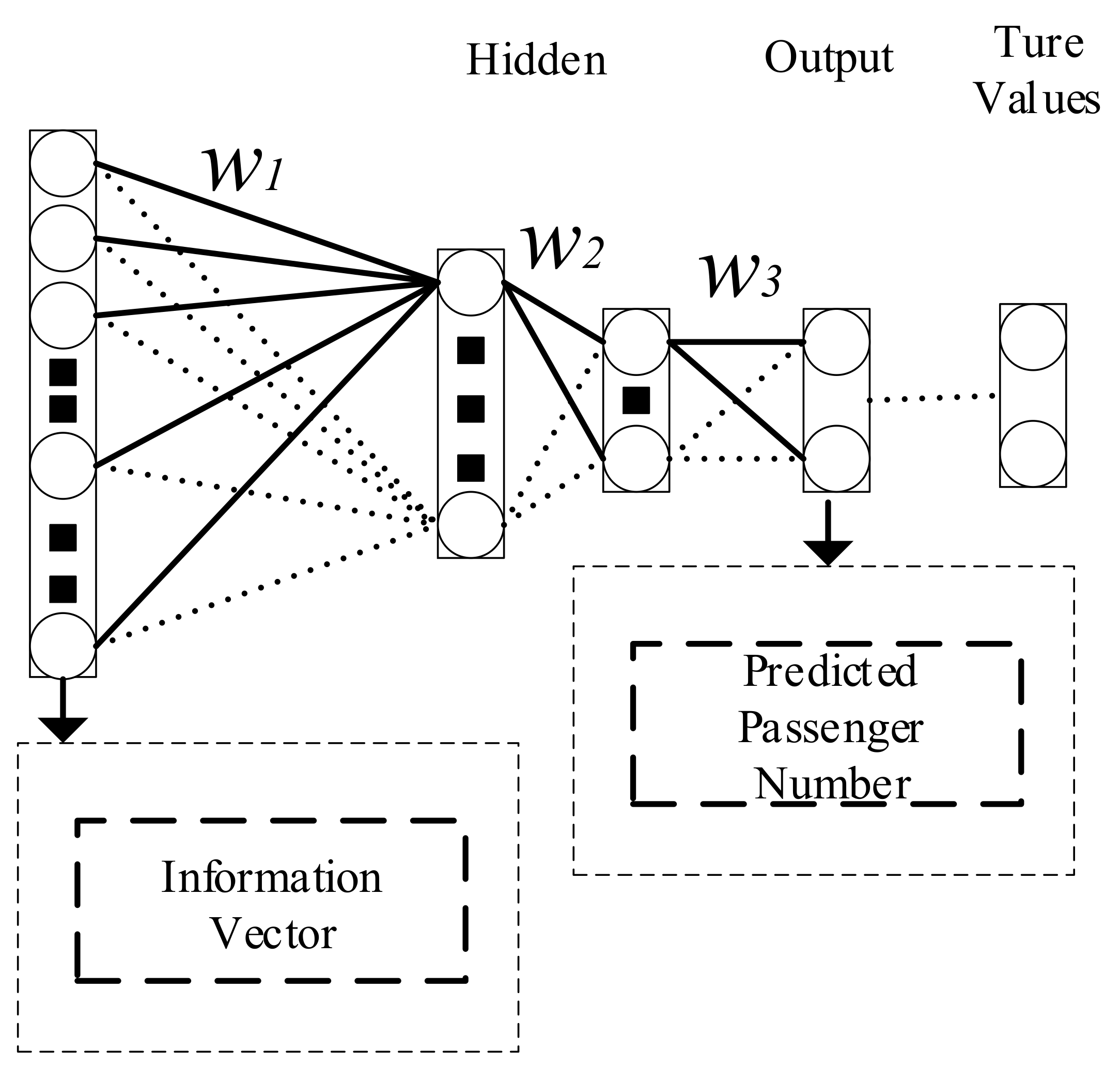
We use a three-layer neural network to decode the information vector. The main function of the first hidden layer is information focusing, namely reducing the input information dimension through a fully connected layer to increase calculation speed. The connection mode of the second hidden layer is also fully connected, and it is activated by the sigmoid function to complete the linear-to-non-linear conversion. The main role of this layer is to find the non-linear relationship between the data. The main function of the third hidden layer is to decode the information from the first two layers and transform the information into a vector which has the same dimension as real values. The process of the decoding part is shown in Figure 5.

4. Results and Discussion

The train dataset used was extracted from October 1, 2015 to October 25, 2015. The test dataset was from October 26, 2015 to October 30, 2015. The two lines were 685 and 56008. Line 56008 has a large passenger volume, because it is a major bus line on the third ring road. Line 685 is a normal line which has a relatively small passenger volume. We chose these two lines to evaluate the performance of the HRPFP model in different scales. These two lines are shown in Figure 6.
Here, we chose the root mean square error (RMSE) as an evaluation for the service radius configuration part. The RMSE can be calculated by Equation (19).
RMSE = 1 M m = 1 M y m y m ^ 2
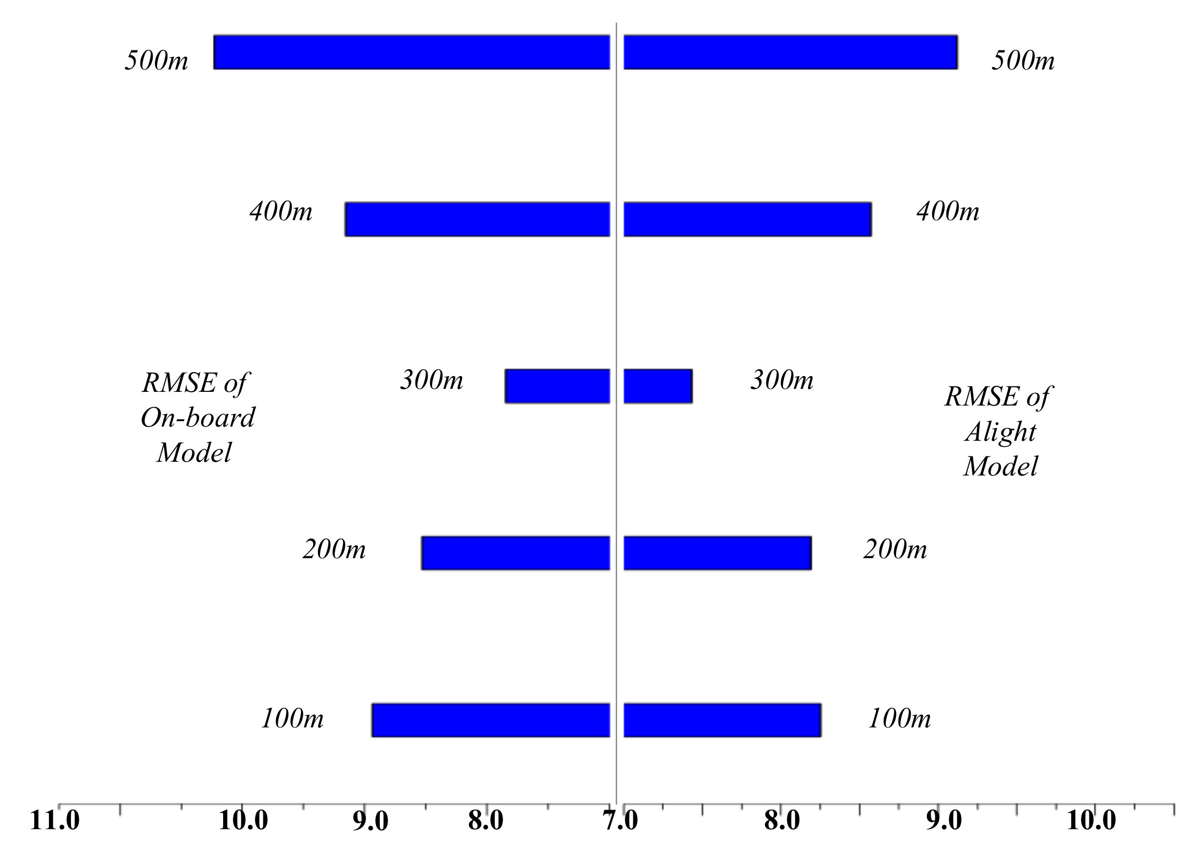
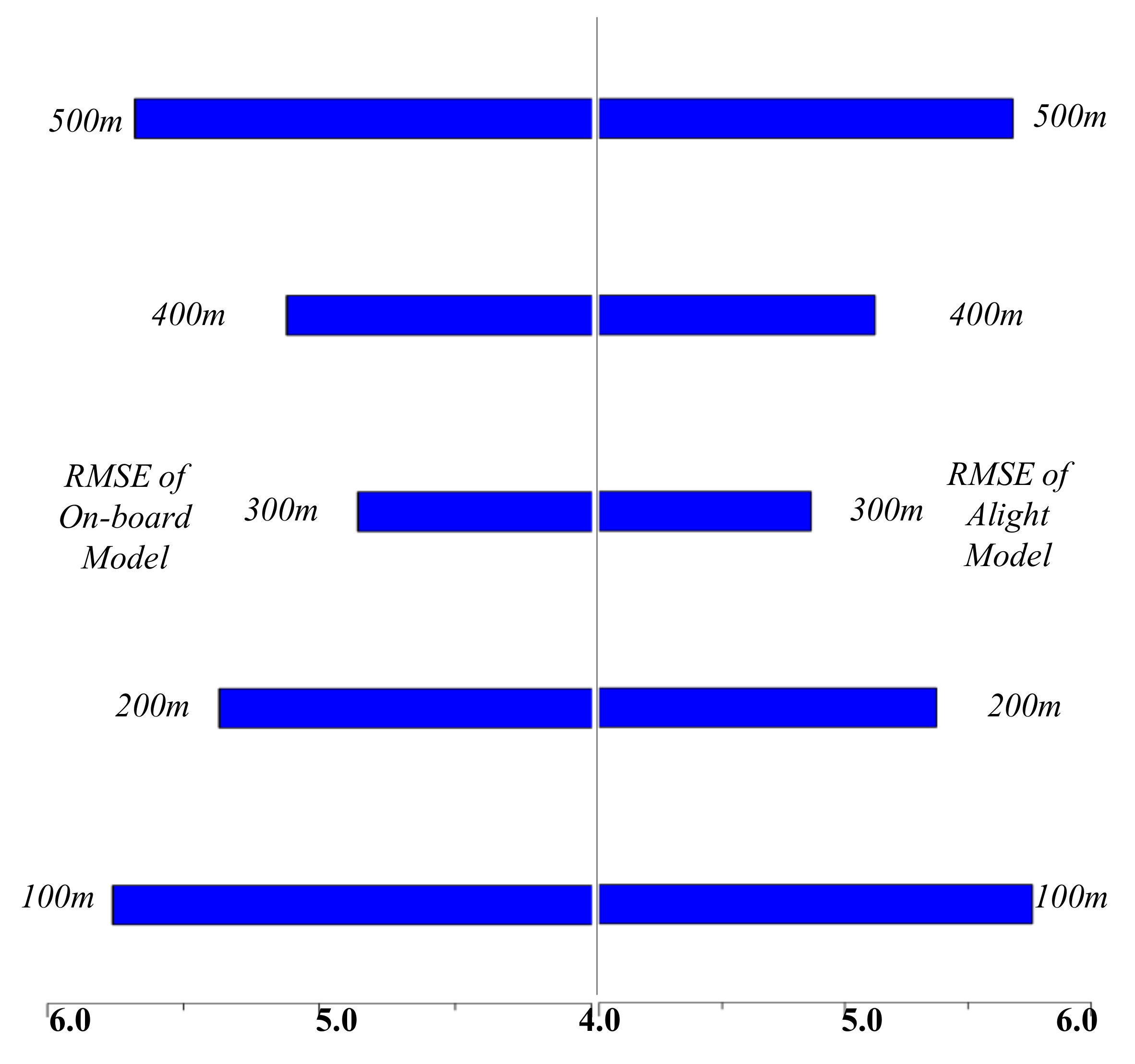
where M is the total number of samples, y m is the true value, and y m ^ is the predicted value. For line 56008, the optimal parameters of the predicted model are as follows: the maximum tree depth was 4 layers, the learning rate was 0.02, the maximum tree size was 1500, and the optimal distance was 300 m. For line 685, the maximum tree depth was 3 layers, the learning rate was 0.01, the maximum size of the tree was 800, and the optimal distance was 300 m. The evaluation of prediction model for line 56008 under different distances is shown in Figure 7. When the distance was 500 m, the RMSE of these models was close to 10, and when the distance was 300 m, the RMSE of the passenger flow prediction models was about 7.7. The evaluation of the prediction model for line 685 under different distances is shown in Figure 8. When the distance was 100 m, the RMSE of these models was the largest which was close to 5.5, and when the distance was 300 m, the RMSE of the passenger flow prediction models was about 4.5.
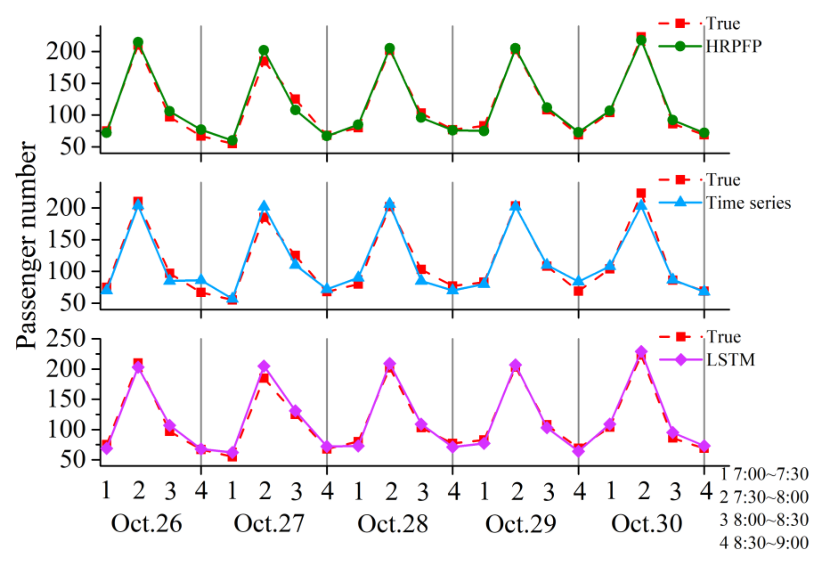
Through analysis, it can be found that if the input of real-time data encoding part was set to a vector 0, the model will be transformed to a LSTM sequence model. In order to verify the performance of the HRPFP model, we selected the time series and the LSTM model as comparison. The two selected stations were the major on-board stations of line 56008 and line 685. The major on-board station of line 56008 was the 8th station. During the test date, the predicted passenger number of different models from 7:00 to 9:00 are shown in Figure 9. We can see that the predicted values of time series model were around the history average value and presented an obvious periodic characteristic. The predicted values of the LSTM model and the HRPFP model varied among different days, which meant that these two models can reflect the daily passenger flow trend. The HRPFP model performed better than the LSTM and time series models in this station.
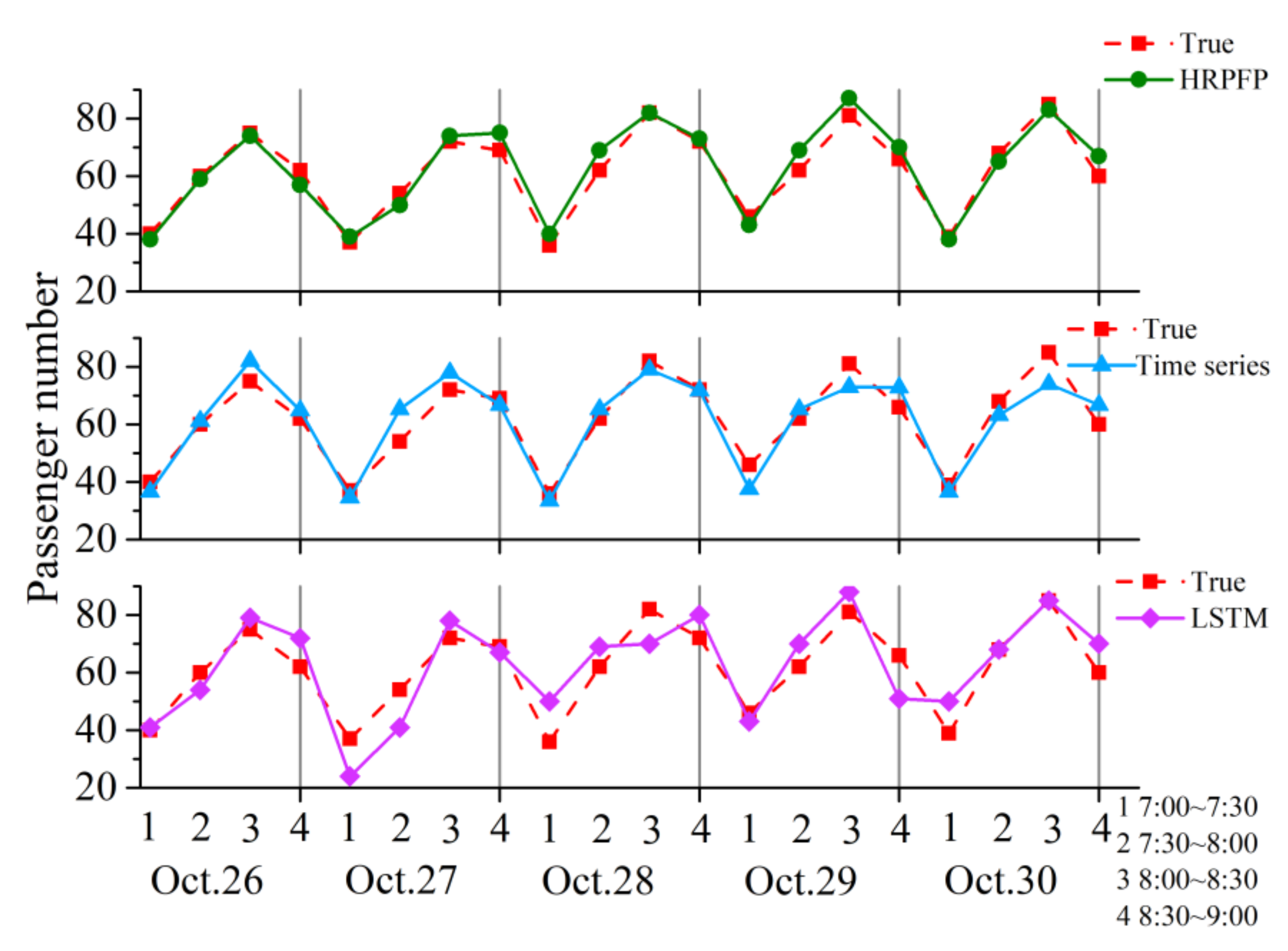
In the same time periods, the predicted passenger number using different models for the major on-board station (the 7th station) of line 685 are shown in Figure 10. Due to the passenger number being small at this station, the passenger data fluctuated strongly. Therefore, the time series model cannot find this regularity effectively. The LSTM model can only find part of this regularity. The HRPFP model was more accurate than the other two models due to the addition of POI features and, especially, the real-time data information.
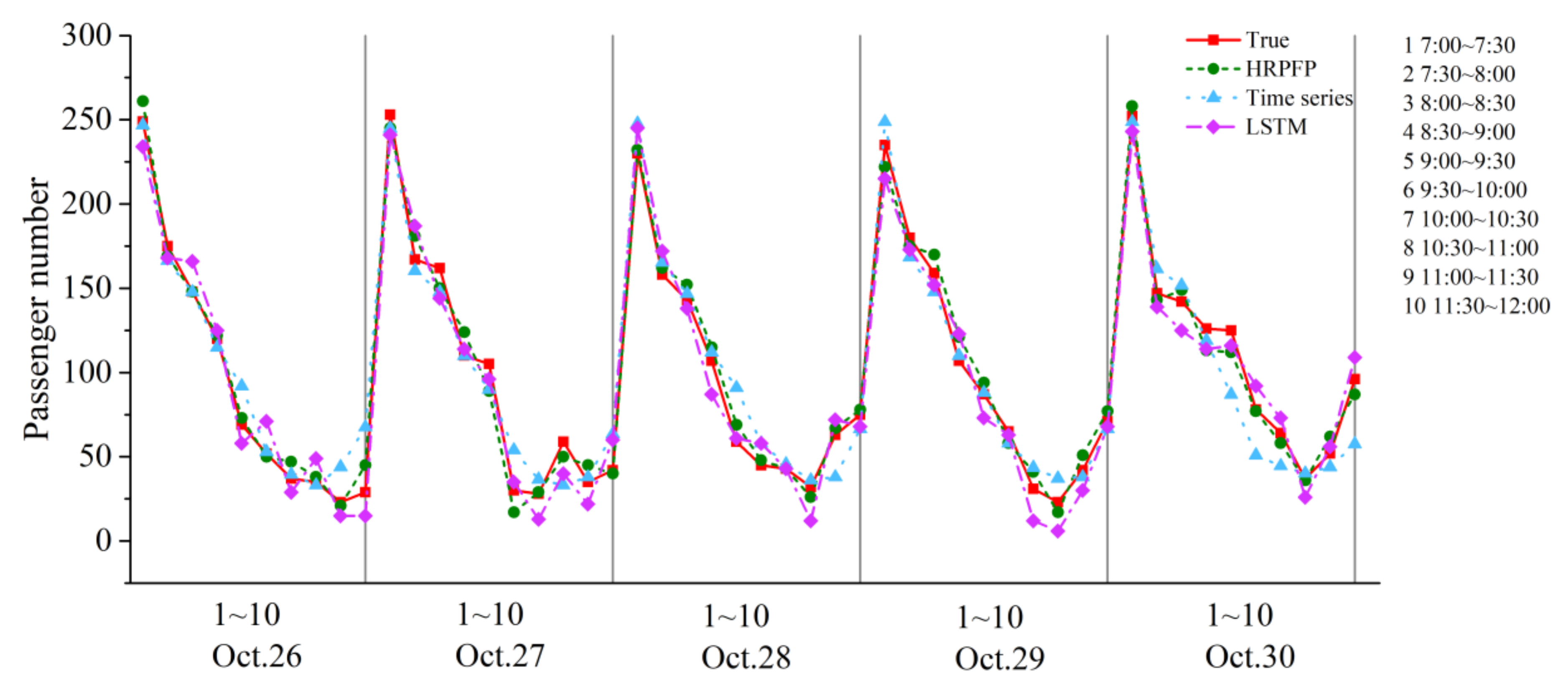
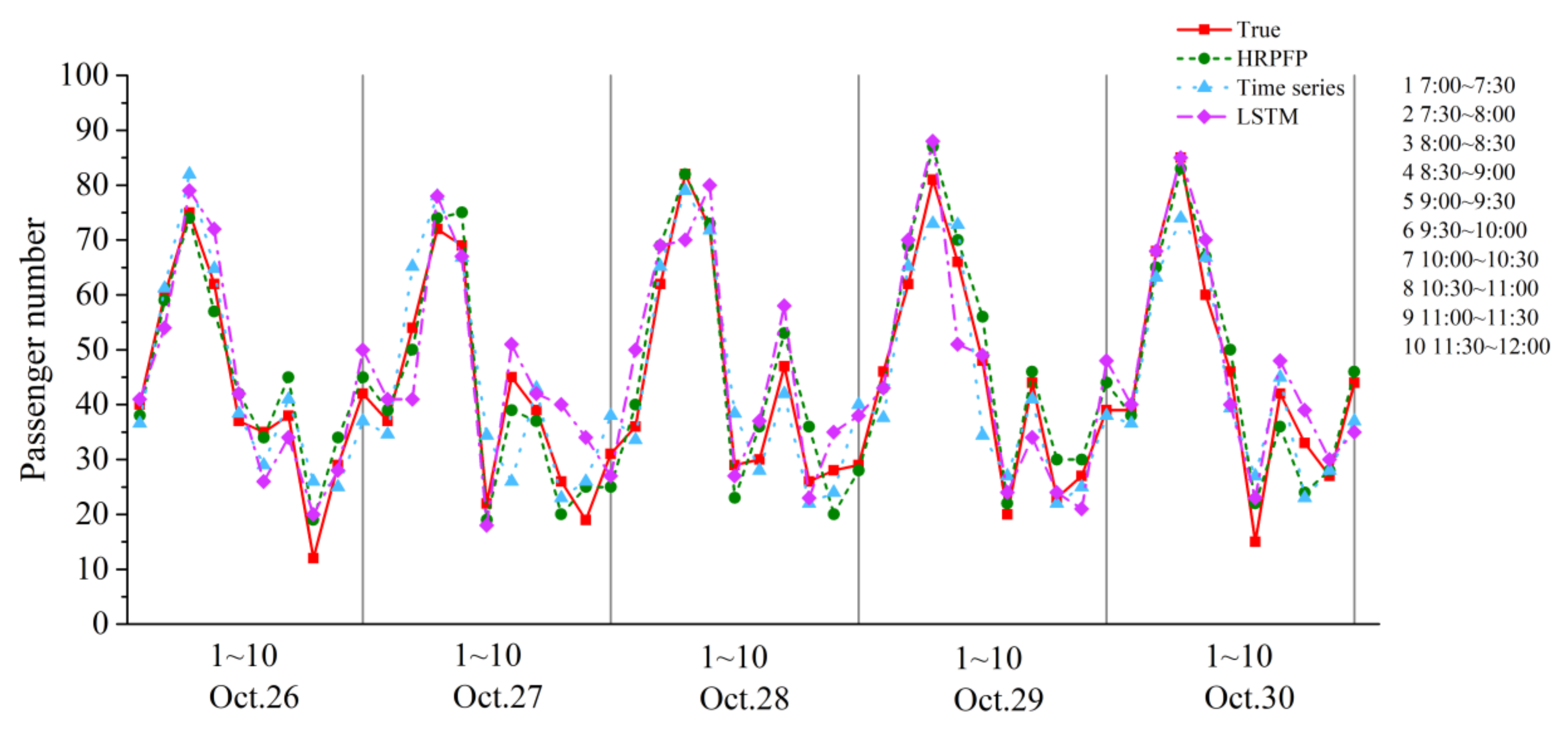
We extended the time period to 7:00~12:00. From Figure 11, we can see that due to the irregular fluctuation of daily passenger flow from 10:00 to 12:00, the performance of the HRPFP model was significantly better than the LSTM model and the time series model at the 8th station in line 56008. The performance of the HRPFP model was also the best at the 7th station in line 685, as shown in Figure 12. However, the time series model performed a bit better than the LSTM model at the 7th station in line 685. We believed the major reason for this phenomenon was that the changing amplitude of the passenger flow at this station was smaller than that at the 8th station in line 56008, and the LSTM model overfitted.
Besides the comparison with these two sequence models at a certain station, we also compared the HRPFP model with the Xgboost model and the SVM model in bus passenger flow prediction for the lines. Using the time series model in passenger number prediction for the lines required establishing a prediction model for each site. The organization process of the time series model was too complicated, so we did not choose the time series model as a baseline in bus passenger flow prediction for the lines. Besides RMSE, we also used MAE and MaxError as the evaluation for different methods. The MAE can be calculated by Equation (20).
MAE = 1 M m = 1 M y m y m ^
MaxError = max y m y m ^   m M
where M is the total number of samples, y m is the true value, and y m ^ is the predicted value. The MaxError can be calculated by Equation (21). We used the MaxError as one of our evaluation standards because usually the SVM model has a greater error in the station with a large passenger number. However, these stations have a great meaning for bus operations, and we cannot ignore this error. From Table 1, we can see that the LSTM and HRPFP had a smaller MaxError than the other two methods. The performance of the HRPFP model was the best for both line 56008 and line 685.
We also analyzed the sensitivity of each model mentioned above. The sensitivity analysis experiment was based on the real data on Oct. 27th, 2015. We assumed that the passenger flow data of the 8th station for line 56008 from 7:00 to 8:00 had changed a little based on the real value, then we can recalculate the predicted passenger number of different models based on this change. The results are shown in Table 2. It can be seen that the LSTM model indexed by the date was the least sensitive on passenger flow prediction, and the predicted value did not change as the real-time data changed. The SVM model and the Xgboost model changed slightly. The predicted value of the HRPFP model will change significantly as the data updated. Therefore, the HRPFP model is more sensitive to real-time data. When passenger number changed at a certain time period suddenly, the HRPFP model will reflect this change, which means that the HRPFP model performs better in real-time passenger flow prediction.

5. Conclusions

Based on the LSTM structure, this paper proposes a new passenger flow prediction model that considers real-time data. This model combines point of interest data with smart card data to improve the dimension of dataset. Then, we use the date as an index of LSTM structure to produce a history information vector. Furthermore, the time section is used as an index of LSTM structure to produce a real-time information vector. With the help of these two information vectors, we can predict bus passenger number more accurately after a decoding process. By comparing with different models, the HRPFP model has a higher accuracy than other models in passenger flow prediction. Due to the addition of the real-time encoding part, the HRPFP model has a better sensitivity to real-time data. Therefore, when a sudden passenger flow change occurs, the HRPFP model can provide an early warning of this phenomenon based on the real-time collected data, provide more accurate data for the adjustment of the bus plan, and make the bus system have a better stability. In the future, we will try to find a more proper sequence length for both the history data encoding part and real-time encoding part to make our research more complete. We hope this research can help bus operations and improve the bus system stability in the future.
Author Contributions

Conceptualization, Q.O.; Methodology, Q.O.; Software, Q.O.; Formal analysis, J.L.; Resources, J.M.; Project administration, Y.L. All authors have read and agree to the published version of the manuscript.

Funding

This research was funded by National Natural Science Foundation of China grant number 61872036 and National key technologies Research & Development program grant number 2017YFC0804900. And the APC was funded by National Natural Science Foundation of China.

Conflicts of Interest

The authors declare no conflict of interest.

References

  1. Milenković, M.; Švadlenka, L.; Melichar, V.; Bojović, N.; Avramović, Z. SARIMA modelling approach for railway passenger flow forecasting. Transport 2018, 33, 1113–1120. [Google Scholar] [CrossRef] [Green Version]
  2. Gummadi, R.; Edara, S.R. Analysis of Passenger Flow Prediction of Transit Buses along a Route Based on Time Series. In Information and Decision Sciences; Springer: Berlin/Heidelberg, Germany, 2018; pp. 31–37. [Google Scholar]
  3. Ni, M.; He, Q.; Gao, J. Forecasting the subway passenger flow under event occurrences with social media. IEEE Trans. Intell. Transp. Syst. 2016, 18, 1623–1632. [Google Scholar] [CrossRef]
  4. Li, C.; Huang, J.; Wang, B.; Zhou, Y.; Bai, Y.; Chen, Y.J.I.A. Spatial-Temporal Correlation Prediction Modeling of Origin-Destination Passenger Flow Under Urban Rail Transit Emergency Conditions. IEEE Access 2019, 7, 162353–162365. [Google Scholar] [CrossRef]
  5. Kumar, S.V. Traffic flow prediction using Kalman filtering technique. Procedia Eng. 2017, 187, 582–587. [Google Scholar] [CrossRef]
  6. Jiao, P.; Li, R.; Sun, T.; Hou, Z.; Ibrahim, A. Three revised Kalman filtering models for short-term rail transit passenger flow prediction. Math. Probl. Eng. 2016, 2016, 9717582. [Google Scholar] [CrossRef] [Green Version]
  7. Tang, M.; Li, Z.; Tian, G. A Data-Driven-Based Wavelet Support Vector Approach for Passenger Flow Forecasting of the Metropolitan Hub. IEEE Access 2019, 7, 7176–7183. [Google Scholar] [CrossRef]
  8. Sun, Y.; Leng, B.; Guan, W. A novel wavelet-SVM short-time passenger flow prediction in Beijing subway system. Neurocomputing 2015, 166, 109–121. [Google Scholar] [CrossRef]
  9. Liu, R.; Wang, Y.; Zhou, H.; Qian, Z. Short-Term Passenger Flow Prediction Based on Wavelet Transform and Kernel Extreme Learning Machine. IEEE Access 2019, 7, 158025–158034. [Google Scholar] [CrossRef]
  10. Li, C.; Wang, X.; Cheng, Z.; Bai, Y. Forecasting Bus Passenger Flows by Using a Clustering-Based Support Vector Regression Approach. IEEE Access 2020, 8, 19717–19725. [Google Scholar] [CrossRef]
  11. Makridakis, S.; Spiliotis, E.; Assimakopoulos, V. Statistical and Machine Learning forecasting methods: Concerns and ways forward. PLoS ONE 2018, 13, e0194889. [Google Scholar] [CrossRef] [PubMed] [Green Version]
  12. Guo, J.; Xie, Z.; Qin, Y.; Jia, L.; Wang, Y. Short-term abnormal passenger flow prediction based on the fusion of SVR and LSTM. IEEE Access 2019, 7, 42946–42955. [Google Scholar] [CrossRef]
  13. Toqué, F.; Khouadjia, M.; Come, E.; Trepanier, M.; Oukhellou, L. Short & long term forecasting of multimodal transport passenger flows with machine learning methods. In Proceedings of the 2017 IEEE 20th International Conference on Intelligent Transportation Systems (ITSC), Yokohama, Japan, 16–19 October 2017; pp. 560–566. [Google Scholar] [CrossRef]
  14. Sunardi, S.; Dwiyanto, D.; Sinambela, M.; Jamaluddin, J.; Manalu, D.R. Prediction of Domestic Passengers at Kualanamu International Airport Using Long Short Term Memory Network. MEANS 2019, 4, 165–168. [Google Scholar]
  15. Liu, Y.; Liu, Z.; Jia, R. DeepPF: A deep learning based architecture for metro passenger flow prediction. Transp. Res. Part C Emerg. Technol. 2019, 101, 18–34. [Google Scholar] [CrossRef]
  16. Huang, Z.; Li, Q.; Li, F.; Xia, J. A Novel Bus-Dispatching Model Based on Passenger Flow and Arrival Time Prediction. IEEE Access 2019, 7, 106453–106465. [Google Scholar] [CrossRef]
  17. Han, Y.; Wang, C.; Ren, Y.; Wang, S.; Zheng, H.; Chen, G. Short-Term Prediction of Bus Passenger Flow Based on a Hybrid Optimized LSTM Network. ISPRS Int. J. Geo-Inf. 2019, 8, 366. [Google Scholar] [CrossRef] [Green Version]
  18. Zhang, J.; Shen, D.; Tu, L.; Zhang, F.; Xu, C.; Wang, Y.; Li, Z. A real-time passenger flow estimation and prediction method for urban bus transit systems. IEEE Trans. Intell. Transp. Syst. 2017, 18, 3168–3178. [Google Scholar] [CrossRef]
  19. Pasini, K.; Khouadjia, M.; Same, A.; Ganansia, F.; Oukhellou, L. LSTM Encoder-Predictor for Short-Term Train Load Forecasting; Springer: Berlin/Heidelberg, Germany, 2019. [Google Scholar]
  20. Farahani, M.; Farahani, M.; Manthouri, M.; Kaynak, O. Short-Term Traffic Flow Prediction Using Variational LSTM Networks. arXiv 2020, arXiv:2002.07922. [Google Scholar]
  21. Chen, T.; Guestrin, C. XGBoost: A Scalable Tree Boosting System. In Proceedings of the ACM SIGKDD International Conference on Knowledge Discovery & Data Mining, San Francisco, CA, USA, 13–17 August 2016. [Google Scholar]
  22. Hochreiter, S.; Schmidhuber, J. Long Short-term Memory. Neural Comput. 1997, 9, 1735–1780. [Google Scholar] [CrossRef] [PubMed]
Figure 1. The basic LSTM cell.
Applsci 10 03788 g001
Figure 2. The structure of the HRPFP model.
Applsci 10 03788 g002
Figure 3. The process of the best service radius configuration.
Applsci 10 03788 g003
Figure 4. The process of the history and real-time data encoding.
Applsci 10 03788 g004
Figure 5. The process of the information decoding.
Applsci 10 03788 g005
Figure 6. The two lines (line 56008 and line 685) used in this research.
Applsci 10 03788 g006
Figure 7. The RMSE and distance of the best service radius configuration part in the HRPFP model for line 56008.
Applsci 10 03788 g007
Figure 8. The RMSE and distance of the best service radius configuration part in the HRPFP model for line 685.
Applsci 10 03788 g008
Figure 9. The comparison of three methods in passenger flow prediction using data from 7:00 to 9:00 for the 8th station in line 56008.
Applsci 10 03788 g009
Figure 10. The comparison of three methods in passenger flow prediction using data from 7:00 to 9:00 for the 7th station in line 685.
Applsci 10 03788 g010
Figure 11. The comparison of three methods in passenger flow prediction using data from 7:00 to 12:00 for the 8th station in line 56008.
Applsci 10 03788 g011
Figure 12. The comparison of three methods in passenger flow prediction using data from 7:00 to 12:00 for 7th station in line 685.
Applsci 10 03788 g012
Table 1. Evaluation values of different models for on-board passenger number prediction.
ModelLine 56008Line 685
RMSEMAEMaxErrorRMSEMAEMaxError
HRPFP7.987.53124.694.248
LSTM8.398.13125.324.468
Xgboost9.168.62205.764.7410
SVM9.869.58436.094.9021
Table 2. A simple case of the 8th station in line 56008 on the sensitivity of different models.
Input ValuesPredicted Values from 8:00 to 8:30
Passenger Number from 7:00 to 7:30Passenger Number from 7:30 to 8:00HRPFPLSTMXGBOOSTSVM
235180170152149145
245190181152150146
255200194152150146
265210195152152148
275220212152153148