Article

Retrieval of Turbidity on a Spatio-Temporal Scale Using Landsat 8 SR: A Case Study of the Ramganga River in the Ganges Basin, India

1
State Environment Protection Key Laboratory of Satellite Remote Sensing, Aerospace Information Research Institute, Chinese Academy of Sciences, Beijing 100101, China
2
Environment & Climate Change Research Institute, National Water Research Center, El-Qanater El-Khairiya 13621/5, Egypt
3
Department of Hydrogeology, King Abdulaziz University, Jeddah 21589, Saudi Arabia
4
Department of Earth Sciences, Indian Institute of Technology Roorkee, Roorkee 247667, India
*
Authors to whom correspondence should be addressed.
Appl. Sci. 2020, 10(11), 3702; https://doi.org/10.3390/app10113702
Submission received: 26 April 2020 / Revised: 19 May 2020 / Accepted: 20 May 2020 / Published: 27 May 2020
(This article belongs to the Special Issue Effects of Mineral Elements on the Environment)

Abstract

:
Nowadays, space-borne imaging spectro-radiometers are exploited for many environmental applications, including water quality monitoring. Turbidity is a standout amongst the essential parameters of water quality that affect productivity. The current study aims to utilize Landsat 8 surface reflectance (L8SR) to retrieve turbidity in the Ramganga River, a tributary of the Ganges River. Samples of river water were collected from 16 different locations on 13 March and 27 November 2014. L8SR images from 6 March and 17 November 2014 were downloaded from the United States Geological Survey (USGS) website. The algorithm to retrieve turbidity is based on the correlation between L8SR reflectance (single and ratio bands) and insitu data. The b2/b4 and b2/b3 bands ratio are proven to be the best predictors of turbidity, with R2 = 0.560 (p < 0.05) and R2 = 0.726 (p < 0.05) for March and November, respectively. Selected models are validated by comparing the concentrations of predicted and measured turbidity. The results showed that L8SR is a promising tool for monitoring surface water from space, even in relatively narrow river channels, such as the Ramganga River.

1. Introduction

Turbidity is animportant parameter for water quality and a surrogate for the transparency of water [1,2,3,4,5]. Turbidity can damage many aquatic organisms and fishes by degrading spawning grounds, reducing feed supplies, and affecting gill function [6]. A decrease or increase in water transparency can adversely affect the organic components of systems that adjustto light-dispersing environments [7,8,9,10,11,12,13,14,15]. In estuarine waters with high turbidity, dissolved oxygen concentrations can significantly decrease due to irregularities in heterotrophic and autotrophic processes, which may contribute to the depletion ofmarine organisms [16,17]. Typically, turbidity is assessed visually using aSecchi disk, or presumably through nephelometry [1,5]. However, these methods only represent the locations from which the sample was collected. Recently, remote sensing of sea color has become a valuable method to retrieve and monitor suspended sediment concentration (SSC) and turbidity in coastal turbid waters on the surface [18,19,20,21]. Traditional water quality sampling is cost-effective and time-consuming, as it involves the collection and analysis of the water. Also, the traditional method of water monitoring does not provide the spatial or temporal view of the entire body of water that is necessary for proper management [22].
The use of remote sensing technology to analyze water quality is concise; it alsocaptures the entire field of study to create consistent surface data and periodically demonstrate the point-by-point spatial variability of water quality [23]. Although research on various remote sensing technologies is devoted to total SSC retrieval, research on retrieving turbidity is limited [21]. Even thoughsatellite remote sensing cannot identify near-bed absorption, it is used to identify spatial and temporal variations in turbidity at the surface.“Near-bed absorption” refers to the bottom of a stream or other body of water. The turbidity of the surface water can influence the reflection of the water body, but not from the bottom of the stream/lake/ocean, because the reflection data are obtained from the top 2 m of surface water [24].
The Ramganga River is an important tributary of the Ganges River. It originates from the lower Himalayas in Uttarakhand, covering the vast Ganga Flood Plains (GFP) of Uttar Pradesh, and then converges with the Ganges River. It is the primary source of water for the Jim Corbett National Park (Tiger Reserve) situated in the Uttarakhand, and is one of the critical water sources for domestic, industrial, and agricultural use in the western Uttar Pradesh [25,26]. The upper reaches of the study area consist of hillocks and streams, while agricultural fields mainly dominate the middle and lower reaches; therefore, when sufficient rainfall increases the contribution of suspended substances, due to weathering and erosion processes in the upper regions and agricultural runoff in the middle and lower regions, the turbidity and total SSC increase considerably [27]. The aquatic life of the Ramganga River is negatively affected by the large amount of turbidity in the water, and harmful bacteria and pollutants may also be associated with the particles that cause turbidity. Estimating turbidity distribution in the Ramganga River with diverse geomorphology and a complex environment requires anunconventional approach. Remote sensing technology provides reliable information for monitoring and understanding the variation of turbidity in time and space, particularly in the substantial zone with limited access, such as Jim Corbett National Park area of the Ramganga River Basin.
Mapping turbidity and other indicators of water quality is routinely performed using information acquired with wide-swath imagingspectro-radiometers designed to measure sea color—for example, Orbview-2/SeaWiFS, ENVISAT/MERIS, and Aqua/MODIS [28]. However, these applications are not suitable for narrow and small regions, due to their low spatial resolution scales, yielding a large number of mixed pixels and resulting in lower accuracy of retrievals [29]. In comparison to these medium resolution images, Landsat 8 surface reflectance (L8SR) images aredelivered on a Polar Stereo (PS) or universal transverse Mercator (UTM) mapped grid with 30 m spatial resolution.
Table 1 shows the important features of the L8SR product. Various surveys of remote detection of ocean color were carried out to retrieve water quality parameters, most of which used three basic strategies: (i) implicit, based on the correlation between water quality parameters, using inherent optical properties (IOPs) and semi-analytical models [30,31,32]; (ii) using experimental models between these parameters and IOPs [33,34]; and (iii) experimental models using water quality parameters and satellite data reflection [35,36,37,38]. The third approach was used in this study, which is based on the correlation between field measurements and reflectance values extracted from L8SR products.

2. Materials and Methods

2.1. Study Area

Ramganga River flows through the Himalayas (Kumaon region) in Uttarakhand and the GFP before joining the Ganges River in Uttar Pradesh. The river has a catchment area of approximately 22,685 km2, with a total stretch of 642 km from its origin (Dudhotali Mountain of the district Chamoli) to the confluence with the Ganges River [39,40,41,42]. The Ramganga River catchment lies between 30°06′02.22″ N to 27°10′42.11″ N and 79°16′59.22″ E to 79°50′16″ E, with a mean elevation of 1530 m above mean sea level. After covering the first 158 km of its stretch in the Kumaon Himalayas and going through the Jim Corbett National Park, the river enters the GFP at Kalagarh town, where the Ramganga Dam has been constructed. In the GFP, the river flows through the hugely populated and highly agricultural and industrialized districts of the Uttar Pradesh, such as Moradabad, Bijnor, Bareilly, Rampur, Hardoi, Shahjahanpur, and Farrukhabad [43].

2.1.1. Climatic Condition and Rainfall

Summer, rainy, and winter arethe three distinct seasons witnessed by the study area. The rainy season begins by the middle of June and continues to September or mid-October. Following a brief spell of autumn starting in mid-October, when the temperature drops drastically, the winter season begins in November. October/November and May/June are considered to be thepost-monsoon and pre-monsoon seasons, respectively. Throughout the winter months, some occasional showers also occur (http://indiawaterportal.org/). The average yearly rainfall receives by the area is around 1000 mm [28]. The relationship between water discharge (Q) and the SSC in the Ramganga River are shown in Figure 1. It is clear from the figure that there is a direct relation between Q and SSC.

2.1.2. Geology

The entire catchment region is comprised oftwo major lithotectonic zones, namely the Sub-Himalayas and Lesser Himalayas. In the Sub-Himalayas, the major components are siltstone, sandstone, clays, and boulders, with molasse sediments of Mid-Miocene to Pleistocene age. Unfossiliferous sequences of low- to high-grade meta-sediments of the Palaeozoic to Mesozoic age are the major components of the Lesser Himalayas. In general, the important lithologies in the Ramganga basin are (1) calcareous shales and siltstones (Blaini/Infrakrol formations); (2) quartzites (Nagthat and Sandra formations); (3) low-grade metamorphics (phyllites, slates, and schists); (4) limestones (Krol and Deoband formations); and (5) high-grade metamorphics (granite gneisses) [44].
The river emerges in the Ganga alluvial plain, also known as the GFP, after covering a distance of about 158 km in the Kumaon Himalayas. The Ganga alluvial plain is a foreland basin closely linked with the extension of the Himalaya orogenic belt, as demonstratedin Figure 2. The Quaternary lithostratigraphic sequence established in descending order is comprised of the (1) Ganga/Ramganga Recent Alluvium; (2) Ganga/Ramganga Terrace Alluvium; and (3) Varanasi Older Alluvium, with two facies, i.e., sandy facies and silt clay facies.The first two, the Recent and Terrace alluviums, constitute the Newer Alluvium [45].

2.2. Sample Collection and Analysis

Figure 2 shows the locations where water samples were collected from the Ramganga River. Sampling process was done on 13 March and 27 November of the year 2014 (Table 2). Sixteen samples of river water from each location were collected in a five-liter bottle, preserved, and transferred to the laboratory as suggested in Standard Methods for the Examination of Water and Wastewater (APHA), 20th edition [46].
The sample bottles were rinsed with 2% nitric acid in the laboratory, and rinsed twice with water of the river at the time of sampling to avoid contamination. Turbidimeter (HACH instruments) was used to measure the turbidity in NTU of each water sample.

2.3. Satellite Images

It was observed that all the sampling locations occurred in three images (path 145 and rows 139, 140, and 141). The three images cover an area of approximately 180 km east–west to 540 km north–south. There could be significant variability in the atmospheric conditions over such an area, which affects the relationship between the top of the atmospheric reflectance retrieved from the satellite data and the insitu water turbidity. This problem is mitigated by using a single image where 13 of the 16 sampling sites were located. The reflected electromagnetic solar radiation is the basis for the spectral examination of satellite imagery, issued to measure turbidity. Unique signatures and curves are generated, depending on the reflection and absorption at different wavelengths [47,48]. The major errors in the reflected electromagnetic solar radiation remained when retrieving water properties from satellite images. The thirteen samples (RG2–RG14) included in the analysisare located on the image, with path 145 and row 40. Nine samples wereused to retrieve the turbidity model. To validate this model, the measured and predicted turbidity was compared. The four samples that were not included in the model retrieving were used for further validation of the model.

2.4. Statistical Summary of Ramganga River In Situ Measurements

Insitu concentrations of turbidity were measured in both March and November 2014. The distribution of data of turbidity was generally skewed, with low values and without any outliers or very high values (Table 3). Turbidity concentrations ranged between 20.6 and 112.0 NTU with a mean value of 62.467 NTU during March 2014, and between 2.3 and 15.4 NTU with mean value of 7.267 NTU during November 2014.
In general, turbidity concentrations were higher in March than in November (Figure 3 and Figure 4). The SSC depends on the location and time of the year. When matched to the pre-monsoon and post-monsoon data, the SSC values weremuch higher during the monsoon months. Thisis caused by high Q, leading to high rates of weathering and erosion from the catchment and the river channel itself. Pre-monsoon concentrations (March 2014) are consistently higher than the corresponding post-monsoon concentrations (November 2014). Thiscan be attributed to a considerable difference in elevation levels of 530 m (RG4) to 259 m (RG5) from the mean sea level. This elevation difference leads to a decrease in potential energy and an increase in the kinetic energy of the river, thereby increasing the sediment-carrying capacity of the river [16].

2.5. Image Acquisition

In this study, two L8SR images from 6 March and 17 November 2014 were used to retrieve turbidity in the Ramganga River. The selected images, with path 145 and row 40, were downloaded from the United States Geological Survey (USGS) websites (http://earthexplorer.usgs.gov/). Each downloaded image was in a compressed folder containing TIFF images of each band.

2.6. Methodology

2.6.1. Rescaling

Rescaling of original L8SR bands wasapplied, as the range of the data wasfrom −2000–16,000. The valid range of reflectance is between 0–1. The minimum fraction of irradiance to be reflected from any surface should be 0.0 if it is a fully absorbed material, while the maximum fraction is 1.0 if it is a fully reflective material. The data were rescaled for the valid ranges, according to the information (Table 1) by multiplying each band by the scale factor of 0.001.

2.6.2. Masking

Only the river water body should be retained, and the rest needs to be masked. Masking of the water body was difficult, as the river is very narrow and it has many bridges. In addition, some areas of water in the river have been isolated in the form ofoxbow lakesthat appear after a broad meander from the main channel of the river is cut off, creating a free-standing body of water. Imagery masking was performed using version 10.2.2 of ArcGIS software. The river wasidentified by thresholding the images of the spectral reflectance.

2.7. Regression Models

The relationship between the L8SR reflectance and insitu measurements was developed by exploiting a simple linear backward elimination method. The backward elimination method begins with all the variables observed in the model. At each step, the least significant variable is removed. This process continues until there are no more insignificant variables. The user defines the level of significance at which the variables can be removed from the model [49]. In this study, IBM SPSS programming statistics v. 23.0 (Armonk, NY, USA), was used. Figure 5 shows the outline of the methodology applied in the present study. A regression model between the measured turbidity and the surface reflectance was applied. The output model has been validated, and the final results werethematic maps. For March, the regression was determined between the insitu turbidity on 13 March 2014 and the surface reflectance on 6 March 2014, while for November, the regression was between the insitu turbidity on 21 November 2014 and the surface reflectance on 17 November 2014.
Water quality indicators, such as turbidity, chlorophyll, and temperature, as well as suspended matter, have been retrieved from remote sensing, according to [22]. The following four types of expressions have been used to show the general forms of these experimental equations:
Y = A + BX
Y = ABX
Y = A + B lnX
lnY = A + BX
where X is the measurement from remote sensing (i.e., radiance, reflectance, and energy); Y representswater quality parameters; A and B are empirically derived factors; and X could be energy, reflectance, orradiance in a single or two-band ratio. This concept has been adopted by many researchers in the past to retrieve the parameters of water quality; therefore in the present study, we followed the same concept, constructing an algorithm for turbidity retrieval that is dependent on the relationship between L8SR and insitu observation.

3. Results

3.1. Retrieval of Turbidity

Statistical techniques for the derivation of chlorophyll- a (Chl-a) concentration and turbidity have been a common approach, based on the correlation between insitu data and spectral band values. The derived algorithms can provide an adequate estimate of Chl-a concentration [50] and turbidity [51]. These techniques were also adopted in the Ramganga River, in order to combine in situ data with satellite data to retrieve turbidity. The correlation was pursued between the insitu turbidity data and L8SR (single and ratio bands) for March and November 2014. After testing more than 20 band combinations in this correlation analysis, all single bands showed very poor correlation coefficients. Similar results appeared with different band ratios, except for b2/b3 and b2/b4, which produced higher coefficients of determination. The most significant results are presented in Table 4. Our results agree well with the findings of [52,53], who used b2/b3 and b2/b4 for the retrieval of turbidity from surface reflectance.
Using backward linear regression for the March data, all insignificant bands were removed, and the predictive model results were 0.75 and 0.56 for correlation coefficient (R) and R2 values, respectively—whereas, for November, the value of R and R2 were 0.852 and 0.726, respectively. However, the absence of autocorrelation in the residuals was indicated by Durbin–Watson’s statistic (Tables S1 and S2). The description and summary of the final models of water quality parameters are shown in Table 5.

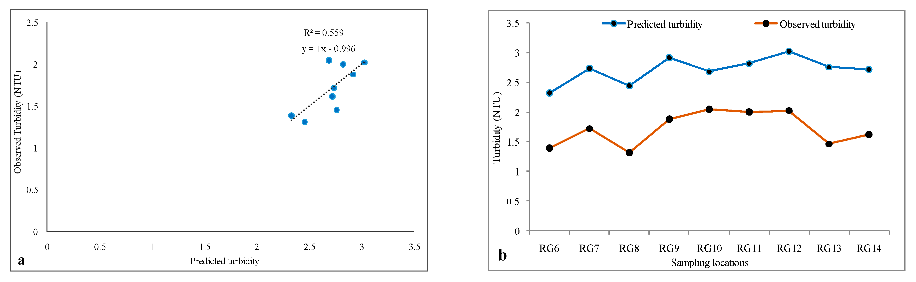
3.2. Algorithm Validation

Comparisons between the measured and predicted turbidity for the nine samples that were used to determine the turbidity model are shown in Figure 6 and Figure 7 and Table S3, along with squared residual and root mean square error (RMSE). Moderate correlation factors(R2) of 0.56 and 0.726, with RMSE 1.013 and 0.178, wereobtained for March and November, respectively. For March, the predicted turbidity ranged from 2.329 to 3.023 NTU in relation to the measured turbidity, which ranged from 1.31 to 2.049 NTU (Figure 6). For November, the predicted turbidity varied from 0.337 to 1.33 NTU, compared with 0.362 to 1.18 NTU for the measured values (Figure 7).

3.3. Additional Validation for the Retrieved Model

For more precision inthe model, the four samples (RG2–RG5), which werenot included in the analysis, wereused to validate the model (Table 6). The first value in March and the last value in November weretoo high, because we tried to collect water samples where the water condition was rather uniform. However, it is still possible that the water samples capture locally high turbidity, while the reflectance of the satellite is on average about 900 m2.
The final turbidity maps, after applying the generated models, are presented in Figure 8 and Figure 9, Figures S1a–c and S2a–c. For March, the estimated concentrations ranged from 2.329 to 3.023 NTU (Figure 8 and Figure S1a–c) in relation to the in situ concentration turbidity, which ranged from 1.31 to 2.049 NTU. For November, the estimated concentrations ranged from 0.337 to 1.33 NTU, compared to 0.362 to 1.18 NTU for the measured values (Figure 9 and Figure S2a–c).

4. Discussion

The main objective of this study was to construct an algorithm to retrieve turbidity in the Ramganga River using L8SR. Statistical techniques [54,55] have been applied to determine the relationship between surface reflectance and measured turbidity. Bands from b1–b5 showed weak correlations for March and November. Different band ratios were utilized—for example, b2/b5, b3/b4, b3/b5, and b4/b5. The b2/b4 ratio was observed to be the most proficient for the estimation of turbidity for March, whereas b2/b3 was the most effective ratio for the estimation of turbidity in November for the Ramganga River. That was because vegetation indices (VIS) (b1, b2, and b3) and near infrared (NIR) (b5) are the most sensitive bands to SSC changes in water surface [56].
Such a monitoring system by remote sensing could be used as an early forewarning system for turbidity exceedance, which could help to make timely decisions about allowed emissions into the river water. Thus, simple and less expensive regular monitoring can be applied at a considerably larger spatial scale than continuous conventional sampling methods. However, errors related to satellite data, which reduce the accuracy of the resulting maps, are as follows:
  • The samples collected may not be representative in relation to the total area of the water body;
  • Water contains many soluble substances that hinder the process ofobtaining the precise signature of the studied parameters;
  • The difference in date between the acquisition of the satellite data and the insitu data;
  • The relatively low spatial resolution of satellite images may affect their accuracy;
  • The uncertainty of the locations of the pixels and insitu samples;
  • The small number of samples affects the regression model, as well as the validation process.
A major problem with medium-resolution satellite data like Landsat 8 is that the Ramganga River is irregular in shape, generally narrow (about 100 m wide), and includes small islands. The reflected radiation from the shore and the vegetation near the shore is generally stronger than the radiation from the water. Therefore, the retrieval water quality parameters might not be possible if even a small portion of a pixel is covered with land. Also, the distinguished turbidity models are probably not relevant for different streams, and are along these site-specific lines. In all cases, testson freshwater bodies with comparable attributes should be undertaken to access the suitability of the models.

5. Conclusions

To retrieve surface turbidity from the L8SR product, a regional algorithm was developed and used in the Ramganga River. This investigation suggests that satellite information can be a ground-breaking device to foresee the concentration of turbidity in stream waters, and particularly in the Ramganga River. However, the distinguished models would be efficient only in the Ramganga River or rivers with comparable water quality and morphological characteristics. Nevertheless, even with the existence of a lot of ground information similar to the case in our examination, a quantitatively accurate estimation of water quality components in inland waters is a great challenge. Using the data acquired byvarious other sensors, such as Sentinel 2, Moderate Resolution Imaging Spectroradiometer (MODIS), and Gaofen-3 (GF-3),can help improve our ability to correctly estimate surface water characteristics from space.

Supplementary Materials

The following are available online at https://www.mdpi.com/2076-3417/10/11/3702/s1, Figure S1a: Turbidity map of Ramganga River in 6 March 2014, Figure S1b: Turbidity map of Ramganga River in 6 March 2014, Figure S1c: Turbidity map of Ramganga River in 6 March 2014, Figure S2a: Turbidity map of Ramganga River in 11 November 2014, Figure S2b: Turbidity map of Ramganga River in 11 November 2014, Figure S2c: Turbidity map of Ramganga River in 11 November 2014, Table S1: Models’ summary and regression analysis statistics among turbidity concentrations and surface reflectance values for March and November 2014 (dependent variable), Table S2: Variables entered/removed from turbidity predictive models relying upon the regression method utilized for March and November 2014, Table S3: Comparison of satellites retrieved and in-situ observed turbidities values at 9 sampling sites of Ramganga River in March and November 2014 with statistical analysis for squared residual, root mean square (RMSE).

Author Contributions

Software: M.A. and M.Y.A.K.; Writing M.A. and M.Y.A.K.; revision and final editing: M.A., Q.M. and M.Y.A.K.; remote sensing and GIS data analysis: M.A. and Q.M.; In-situ data collection and analysis: M.Y.A.K. All authors have read and agreed to the published version of the manuscript.

Funding

This research was funded by the Council for Scientific and Industrial Research (CSIR), New Delhi, grant number 19-06/2011 (i) EU-IV.

Acknowledgments

The authors are also thankful to the National Key Research and Development Program, “Spatial information service and application demonstration of comprehensive monitoring of urban and rural ecological environment” (project number: 2017YFB0503900, 2017YFB0503905); the Major Projects of High Resolution Earth Observation Systems of National Science and Technology (05-Y30B01-9001-19/20-1); and the Science and Technology Cooperation Project of Sanya Municipal Institute, “Non-Point Source Pollution Risk Identification and Quantitative Assessment for Surface Water Source Using Remote sensing” (project number: 2018YD10), for their technical support in this study. The authors are also thankful to Council for Scientific and Industrial Research (CSIR), New Delhi, and IIT Roorkee, India for giving a research fellowship (ref. no: 19-06/2011 (i) EU-IV). The authors gratefully acknowledge the comments of the reviewers and the editor, which enormously improved the presentation of the manuscript.

Conflicts of Interest

The authors declare no conflict of interest.

References

  1. Zheng, G.J. Hydrodynamics and Water Quality: Modeling Rivers, Lakes, and Estuary; John Wiley & Sons, Inc.: Hoboken, NJ, USA, 2007; pp. 130–134. [Google Scholar]
  2. Güttler, F.N.; Niculescu, S.; Gohin, F. Turbidity retrieval and monitoring of Danube Delta waters using multisensor optical remote sensing data: An integrated view from the delta plain lakes to the western–northwestern Black Sea coastal zone. Remote Sens. Environ. 2013, 132, 86–101. [Google Scholar] [CrossRef] [Green Version]
  3. Zablotskii, V.R.; Le, T.G.; Dinh, T.T.H.; Le, T.T.; Trinh, T.T.; Nguyen, T.T.N. Estimation of suspended sediment concentration using vnredsat–1A multispectral data, a case study in red river, hanoi, vietnam. Geogr. Environ. Sustain. 2018, 11, 49–60. [Google Scholar]
  4. Chalov, S.; Golosov, V.; Tsyplenkov, A.; Theuring, P.; Zakerinejad, R.; Märker, M.; Samokhin, M. A toolbox for sediment budget research in small catchments. Geogr. Environ. Sustain. 2017, 10, 43–68. [Google Scholar] [CrossRef] [Green Version]
  5. Chen, S.; Fang, L.; Zhang, L.; Huang, W. Remote sensing of turbidity in seawater intrusion reaches of Pearl River Estuary–A case study in Modaomen water way, China. Estuar. Coast. Shelf Sci. 2009, 82, 119–127. [Google Scholar] [CrossRef]
  6. Minnesota Pollution Control Agency. Turbidity: Description, Impact on Water Quality, Sources, Measures—A General Overview, USA. 2008. Available online: https://www.pca.state.mn.us/sites/default/files/wq-iw3-21.pdf (accessed on 25 June 2019).
  7. Kumar, A.; MMS, C.P.; Chaturvedi, A.K.; Shabnam, A.A.; Subrahmanyam, G.; Mondal, R.; Yadav, K.K. Lead Toxicity: Health Hazards, Influence on Food Chain, and Sustainable Remediation Approaches. Int. J. Environ. Res. Public Health 2020, 17, 2179. [Google Scholar] [CrossRef] [PubMed] [Green Version]
  8. Mishra, S.; Kumar, A. Estimation of physicochemical characteristics and associated metal contamination risk in river Narmada, India. Environ. Eng. Res. 2020, 26, 190521. [Google Scholar] [CrossRef]
  9. Kumar, A.; Sharma, M.P.; Yang, T. Estimation of carbon stock for greenhouse gas emissions from hydropower reservoirs. Stoch. Environ. Res. Risk Assess. 2018, 32, 3183–3193. [Google Scholar] [CrossRef]
  10. Aksnes, D.L.; Dupont, N.; Staby, A.; Fiksen, Ø.; Kaartvedt, S.; Aure, J. Coastal water darkening and implications for mesopelagic regime shifts in Norwegian fjords. Mar. Ecol. Prog. Ser. 2009, 387, 39–49. [Google Scholar] [CrossRef]
  11. Carson, A.B.; Benjamin, M.J.; Krista, K.B.; Daniel, B.Y.; Christian, E.Z. Reconstructing turbidity in a glacially influenced lake using the Landsat TM and ETM+ surface reflectance climate data record archive, Lake Clark, Alaska. Remote Sens. 2015, 7, 13692–13710. [Google Scholar]
  12. Khan, M.Y.A.; Gani, K.M.; Chakrapani, G.J. Assessment of surface water quality and its spatial variation. A case study of Ramganga River, Ganga Basin, India. Arab. J. Geosci. 2016, 9, 28. [Google Scholar]
  13. Khan, M.Y.A.; Khan, B.; Chakrapani, G.J. Assessment of spatial variations in water quality of Garra River at Shahjahanpur, Ganga Basin, India. Arab. J. Geosci. 2016, 9, 516. [Google Scholar] [CrossRef]
  14. Khan, M.Y.A.; Gani, K.M.; Chakrapani, G.J. Spatial and temporal variations of physicochemical and heavy metal pollution in Ramganga River—A tributary of River Ganges, India. Environ. Earth Sci. 2017, 76, 231. [Google Scholar] [CrossRef]
  15. Khan, M.Y.; Hu, H.; Tian, F.; Wen, J. Monitoring the spatio-temporal impact of small tributaries on the hydrochemical characteristics of Ramganga River, Ganges Basin, India. Int. J. River Basin Manag. 2019, 18, 231–241. [Google Scholar] [CrossRef]
  16. Gernez, P.; Barille, L.; Lerouxel, A.; Mazeran, C.; Lucas, A.; Doxaran, D. Remote sensing of suspended particulate matter in turbid oyster farming ecosystems. J. Geophys. Res. Oceans 2014, 119, 7277–7294. [Google Scholar] [CrossRef]
  17. Khan, M.Y.A.; Tian, F. Understanding the potential sources and environmental impacts of dissolved and suspended organic carbon in the diversified Ramganga River, Ganges Basin, India. Proc. Int. Assoc. Hydrol. Sci. 2018, 379, 61–66. [Google Scholar] [CrossRef] [Green Version]
  18. Kumar, A.; Yang, T.; Sharma, M.P. Greenhouse gas measurement from Chinese freshwater bodies: A review. J. Clean. Prod. 2019, 233, 368–378. [Google Scholar] [CrossRef]
  19. Kumar, A.; Sharma, M.P.; Taxak, A.K. Analysis of water environment changing trend in Bhagirathi tributary of Ganges in India. Desal. Water Treat. 2017, 63, 55–62. [Google Scholar] [CrossRef]
  20. Kumar, A.; Sharmab, M.P.; Raic, S.P. A novel approach for river health assessment of Chambal using fuzzy modeling, India. Desal. Water Treat. 2017, 58, 72–79. [Google Scholar] [CrossRef]
  21. Dogliotti, A.I.; Ruddick, K.G.; Nechad, B.; Doxaran, D.; Knaeps, E. A single algorithm to retrieve turbidity from remotely-sensed data in all coastal and estuarine waters. Remote Sens. Environ. 2015, 156, 157–168. [Google Scholar] [CrossRef] [Green Version]
  22. Ritchie, C.J.; Zimba, V.P.; Everitt, H.J. Remote sensing techniques to assess water quality. Photogramm. Eng. Remote Sens. 2003, 69, 695–704. [Google Scholar] [CrossRef] [Green Version]
  23. Allan, M.G.; Hamilton, D.P.; Hicks, B.J.; Brabyn, L. Landsat remote sensing of chlorophyll a concentrations in central North Island lakes of New Zealand. Int. J. Remote Sens. 2011, 32, 2037–2055. [Google Scholar] [CrossRef]
  24. Tassan, S. A procedure to determine the particulate content of shallow water from Thematic Mapper data. Int. J. Remote Sens. 1998, 19, 557–562. [Google Scholar] [CrossRef]
  25. Khan, M.Y.A.; Chakrapani, G.J. Particle size characteristics of Ramganga catchment area of Ganga River. In Geostatistical and Geospatial Approaches for the Characterization of Natural Resources in the Environment; Janardhana, R.N., Ed.; Springer: Cham, Switzerland, 2016; pp. 307–312. [Google Scholar]
  26. Khan, M.Y.A. Spatial variation in the grain size characteristics of sediments in Ramganga River, Ganga Basin, India. In Handbook of Environmental Materials Management; Hussain, C.M., Ed.; Springer: Berlin, Germany, 2018. [Google Scholar]
  27. Khan, M.Y.A.; Daityari, S.; Chakrapani, G.J. Factors responsible for temporal and spatial variations in water and sediment discharge in Ramganga River, Ganga Basin, India. Environ. Earth Sci. 2016, 75, 283. [Google Scholar] [CrossRef]
  28. Vanhellemont, Q.; Ruddick, K. Turbid wakes associated with offshore wind turbines observed with Landsat 8. J. Remote Sens. Environ. 2014, 145, 105–115. [Google Scholar] [CrossRef] [Green Version]
  29. Choodarathnakara, A.L.; Kumar, T.A.; Koliwad, S.; Patil, C.G. Mixed pixels: A challenge in remote sensing data classification for improving performance. Int. J. Adv. Res. Comput. Eng. Technol. (IJARCET) 2012, 1, 261. [Google Scholar]
  30. Kishino, M.; Tanaka, A.; Joji, I. Retrieval of Chlorophyll a, suspended solids, and colored dissolved organic matter in Tokyo Bay using ASTER data. Remote Sens. Environ. 2005, 99, 66–74. [Google Scholar] [CrossRef]
  31. Lim, H.S.; MatJafri, M.Z.; Abdullah, K.; Asadpour, R. A Two-Band algorithm for total suspended solid concentration mapping using theos data. J. Coast. Res. 2012, 29, 624–630. [Google Scholar]
  32. Tebbs, E.J.; Remedios, J.J.; Harper, D.M. Remote sensing of chlorophyll-a as a measure of cyanobacterial biomass in Lake Bogoria, a hypertrophic, saline–alkaline, flamingo lake, using Landsat ETM+. Remote Sens. Environ. 2013, 135, 92–106. [Google Scholar] [CrossRef]
  33. Doxaran, D.; Froidefond, J.M.; Castaing, P.; Babin, M. Dynamics of the turbidity maximum zone in a macrotidal estuary (the Gironde, France): Observations from field and MODIS satellite data. Estuar. Coast. Shelf Sci. 2009, 81, 321–332. [Google Scholar] [CrossRef]
  34. Petus, C.; Chust, G.; Gohin, F.; Doxaran, D.; Froidefond, J.M.; Sagarminaga, Y. Estimating turbidity and total suspended matter in the Adour River plume (South Bay of Biscay) using MODIS 250-m imagery. Cont. Shelf Res. 2010, 30, 379–392. [Google Scholar] [CrossRef] [Green Version]
  35. Ouillon, S.; Douillet, P.; Petrenko, A.; Neveux, J.; Dupouy, C.; Froidefond, J.M.; Andréfouët, S.; Caravaca, A.M. Optical algorithms at satellite wavelengths for Total Suspended Matter in tropical coastal waters. Sensor 2008, 8, 4165–4185. [Google Scholar] [CrossRef]
  36. Tong, P.H.S.; Truong, M.C.; Hoang, C.T. Detecting chlorophyll-a concentration and bloom patterns at upwelling area in South central Vietnam by high resolution multi-satellite data. J. Environ. Sci. Eng. A 2015, 4, 215–224. [Google Scholar]
  37. Ali, P.Y.; Jie, D.; Sravanthi, N. Remote sensing of chlorophyll-a as a measure of red tide in Tokyo Bay using hotspot analysis. J. Remote Sens. Appl. Soc. Environ. 2015, 2, 11–25. [Google Scholar]
  38. Zhang, Y.; Zhang, Y.; Shi, K.; Zha, Y.; Zhou, Y.; Liu, M. A Landsat 8 OLI-Based, semianalytical model for estimating the total suspended matter concentration in the slightly turbid Xin’anjiang reservoir (China). IEEE J. Sel. Top. Appl. Earth Obs. Remote Sens. 2016, 9, 398–413. [Google Scholar] [CrossRef]
  39. Daityari, S.; Khan, M.Y. Temporal and spatial variations in the engineering properties of the sediments in Ramganga River, Ganga Basin, India. Arab. J. Geosci. 2017, 10, 134. [Google Scholar] [CrossRef]
  40. Khan, M.Y.A.; Hasan, F.; Panwar, S.; Chakrapani, G.J. Neural network model for discharge and water-level prediction for Ramganga River catchment of Ganga Basin, India. Hydrol. Sci. J. 2016, 61, 2084–2095. [Google Scholar] [CrossRef] [Green Version]
  41. Khan, M.Y.A.; Hasan, F.; Tian, F. Estimation of suspended sediment load using three neural network algorithms in Ramganga River catchment of Ganga Basin, India. Sustain. Water Resour. Manag. 2019, 5, 1115–1131. [Google Scholar] [CrossRef]
  42. Khan, M.Y.A.; Tian, F.; Hasan, F.; Chakrapani, G.J. Artificial neural network simulation for prediction of suspended sediment concentration in the River Ramganga, Ganges Basin, India. Int. J. Sediment Res. 2019, 34, 95–107. [Google Scholar] [CrossRef]
  43. CWC. Environmental Evaluation Study of Ramganga Major Irrigation Project; Central Water Commission: Uttar Pradesh, India, 2012; Volume 1, p. 16.
  44. Gupta, R.P.; Joshi, B.C. Landslide hazard zoning using the GIS approach—A case study from the Ramganga catchment, Himalayas. Eng. Geol. 1990, 28, 119–131. [Google Scholar] [CrossRef]
  45. Khan, A.U.; Rawat, B.P. Quaternary Geology and Geomorphology of a Part of Ganga Basin in Parts of Bareilly, Badaun, Shahjahanpur and Pilibhit District, Uttar Pradesh; Geological Survey of India (GSI): Kolkata, India, 1992.
  46. American Public Health Association (APHA). Standard Methods for the Examination of Water and Wastewater, 20th ed.; American Public Health Association: Washington, DC, USA, 1998. [Google Scholar]
  47. Islam, M.R.; Yamaguchi, Y.; Ogawa, K. Suspended sediment in the Ganges and Brahmaputra Rivers in Bangladesh: Observation from TM and AVHRR data. Hydrol. Process. 2001, 15, 493–509. [Google Scholar] [CrossRef]
  48. Kaliraj, S.; Chandrasekar, N.; Mages, N.S. Multispectral image analysis of suspended sediment concentration along the Southern coast of Kanyakumari, Tamil Nadu, India. J. Coast. Sci. 2014, 1, 63–71. [Google Scholar]
  49. Borboudakis, G.; Tsamardinos, I. Forward-backward selection with early dropping. J. Mach. Learn. Res. 2019, 20, 276–314. [Google Scholar]
  50. Mayo, M.; Gitelson, A.; Yacobi, Y.Z.; Ben-Avraham, Z. Chlorophyll distribution in lakeKinneret determined from Landsat thematic mapper data. Int. J. Remote Sens. 1995, 16, 175–182. [Google Scholar] [CrossRef]
  51. Fraser, R.N. Hyperspectral remote sensing of turbidity and chlorophyll a among Nebraska Sand Hills lakes. Int. J. Remote Sens. 1998, 19, 1579–1589. [Google Scholar] [CrossRef]
  52. Bande, P.; Adam, E.; Elbasit, M.A.A.; Adelabu, S. Comparing landsat 8 and sentinel-2 in mapping water quality at vaal dam. In Proceedings of the International Geoscience and Remote Sensing Symposium (IGARSS), Valencia, Spain, 22–27 July 2018. [Google Scholar]
  53. Markogianni, V.; Dimitriou, E.; Tzortziou, M. Monitoring of chlorophyll-a and turbidity in Evros River (Greece) using Landsat imagery. In Proceedings of the First International Conference on Remote Sensing and Geoinformation of the Environment (RSCy2013) International Society for Optics and Photonics, Paphos, Cyprus, 8–10 April 2013; Volume 8795, p. 87950R. [Google Scholar]
  54. Lathrop, R.G.; Lillesand, T.M. Use of thematic mapper data to assess water quality in Green Bay and central Lake Michigan. Photogramm. Eng. Remote Sens. 1986, 52, 671–680. [Google Scholar]
  55. Baban, S.M.J. Detecting water quality parameters in the Norfolk Broads, U.K. using Landsat imagery. Int. J. Remote Sens. 1993, 14, 1247–1267. [Google Scholar] [CrossRef]
  56. Yepez, S.; Laraque, A.; Martinez, J.M.; De Sa, J.; Carrera, J.M.; Castellanos, B.; Lopez, J.L. Retrieval of suspended sediment concentrations using Landsat-8 OLI satellite images in the Orinoco River (Venezuela). Comptes Rendus Geosci. 2018, 350, 20–30. [Google Scholar] [CrossRef]
Figure 1. Plot showing relationship between sediment concentration and water discharge in the Ramganga River.
Applsci 10 03702 g001
Figure 2. Map showing the Ramganga River and the locations of samples.
Applsci 10 03702 g002
Figure 3. Frequency graphs showing the turbidity distribution on 13 March (left) and 27 November 2014 (right).
Applsci 10 03702 g003
Figure 4. Box plots showing the spatial variability in turbidity on 13 March and 27 November 2014.
Applsci 10 03702 g004
Figure 5. Flow chart summarizing the approaches followed.
Applsci 10 03702 g005
Figure 6. (a) Scatter plots and (b) line graphs show the comparison of observed and satellite-retrieved turbidity values at nine sampling sites from the Ramganga River in March 2014.
Applsci 10 03702 g006
Figure 7. (a) Scatter plots and (b) line graphs shows the comparison of observed and satellite-retrieved turbidity values at nine sampling sites from the Ramganga River in November 2014.
Applsci 10 03702 g007
Figure 8. Turbidity map of the Ramganga River on 11 March 2014.
Applsci 10 03702 g008
Figure 9. Turbidity map of the Ramganga River on 11 November 2014.
Applsci 10 03702 g009
Table 1. Significant features of Landsat 8 surface reflectance (L8SR) data product.
Band DesignationBand NameData TypeUnitsRangeValid RangeFill ValueSaturate ValueScale Factor
ProductID_sr_band1Band1INT16Reflectance−2000–16,0000–10,000−999920,0000.0001
ProductID_sr_band1Band2INT16Reflectance−2000–16,0000–10,000−999920,0000.0001
ProductID_sr_band2Band3INT16Reflectance−2000–16,0000–10,000−999920,0000.0001
ProductID_sr_band3Band4INT16Reflectance−2000–16,0000–10,000−999920,0000.0001
ProductID_sr_band4Band5INT16Reflectance−2000–16,0000–10,000−999920,0000.0001
ProductID_sr_band5Band6INT16Reflectance−2000–16,0000–10,000−999920,0000.0001
ProductID_sr_band6Band7INT16Reflectance−2000–16,0000–10,000−999920,0000.0001
Table 2. Sampling sites description with insitu concentration of turbidity.
Sample ID LongitudeLatitudeTurbidity (NTU)-March Turbidity (NTU)-November
RG179.32158129.9840174.3100.6
RG279.25543629.7322335.6001.2
RG379.26115329.6967922.8200.5
RG479.09361129.6060470.8880.6
RG578.76116729.4966395.2703.5
RG678.63610829.31443324.60014.2
RG778.64933629.24334752.6008.9
RG878.67908129.12716120.60013.3
RG978.69839429.06813675.90015.4
RG1078.74411128.890639112.0002.5
RG1178.91203128.66856499.9002.3
RG1279.22952828.449917106.0002.9
RG1379.36802828.29472228.9003.2
RG1479.51386128.09422241.7002.7
RG1579.62330827.68198964.5002.1
RG1679.69754427.49798342.5002.4
Table 3. Descriptive statistics values of turbidity in March and November 2014.
ParametersMarch 2014November 2014
Number of Samples99
Mean62.477.27
Standard Error of the Mean12.231.89
Standard Deviation36.705.67
Variance1346.5532.14
Skewness0.270.55
Standard Error of Skewness0.720.72
Kurtosis−1.88−1.92
Standard Error of Kurtosis1.41.4
Range91.413.1
Minimum20.62.3
Maximum112.015.4
Table 4. Correlation between bands and reflectance for March and November 2014.
BandsMarchNovember
b20.051−0.39
b3−0.1410.196
b4−0.2090.069
b5−0.416−0.155
logb20.045−0.402
logb3−0.1530.187
b2b30.581−0.852 **
b2b40.748 *−0.756 *
b2b50.4240.101
b3b40.5230.391
b3b50.3720.360
log(b3/b5)0.3890.280
b4/b3−0.530−0.38
b4/b50.3480.331
b5b4−0.363−0.126
log(b5/b3)−0.389−0.28
log(b5/b4)−0.360−0.236
logb20.045−0.402
logb3−0.1530.187
logb4−0.2110.045
** Correlation is significant at the 0.01 level. * Correlation is significant at the 0.05 level.
Table 5. Statistical summary and description of the final turbidity model that was computed for March and November 2014.
Model RR2Std.Error of the EstimateR2 ChangeDurbin–Waston
March 2014−1.1 + 5.8 (b2/b4)0.750.560.2−0.081.36
November 20143.896 – 4.186 (b2/b3)0.8520.6870.202−0.0021.972
Table 6. Validation of the retrieved model in March and November 2014.
Observed (NTU)Predicted (NTU)Square ResidualRMSE
March 20145.6002.2880310.9692.2
2.8202.144870.456
0.8881.450880.317
5.2705.459010.036
November 20141.22.2041.0081.39044
0.50.8540.125
0.61.3310.535
3.51.36414.562

