Abstract
The whale optimization algorithm (WOA) is a new swarm intelligence (SI) optimization algorithm, which has the superiorities of fewer parameters and stronger searching ability. However, previous studies have indicated that there are shortages in maintaining diversity and avoiding local optimal solutions. This paper proposes a multi-strategy ensemble whale optimization algorithm (MSWOA) to alleviate these deficiencies. First, the chaotic initialization strategy is performed to enhance the quality of the initial population. Then, an improved random searching mechanism is designed to reduce blindness in the exploration phase and speed up the convergence. In addition, the original spiral updating position is modified by the Levy flight strategy, which leads to a better tradeoff between local and global search. Finally, an enhanced position revising mechanism is utilized to improve the exploration further. To testify the superiorities of the proposed MSWOA algorithm, a series of comparative experiments are carried out. On the one hand, the numerical optimization experimental results, which are conducted under nineteen widely used benchmark functions, indicate that the performance of MSWOA stands out compared with the standard WOA and six other well-designed SI algorithms. On the other hand, MSWOA is utilized to tune the parameters of the support vector machine (SVM), which is applied to the fault diagnosis of analog circuits. Experimental results confirm that the proposed method has higher diagnosis accuracy than other competitors. Therefore, the MSWOA is successfully applied as a novel and efficient optimization algorithm.
1. Introduction
Swarm intelligence optimization algorithms (SIOAs) have consistently been one of the popular investigation fields in computer science, artificial intelligence, and machine learning [1,2]. They are many complex and challenging optimization problems existing in these research fields, and the traditional mathematical methods find it difficult to deal with these problems because of non-linearity and multimodality, while SIOAs make use of the stochastic components and are considerably efficient in resolving such issues [3,4], which has caused the research and application boom of SIOAs. Recent years have witnessed a group of SIOAs for mimicking the behaviors of animal groups in nature, such as the artificial fish-swarm algorithm (AFSA, 2002) [5], artificial bee colony algorithm (ABC, 2006) [6], firefly algorithm (FA, 2009) [7], krill herd algorithm (KH, 2012) [8], Drosophila food-search optimization algorithm (DFO, 2014) [9], grey wolf optimizer (GWO, 2014) [10], moth-flame optimization algorithm (MFO, 2015) [11] and so on. These SIOAs have exhibited great potential to address engineering problems, with no exception to the field of analog circuit fault diagnosis.
As electronic systems have found their way into military, medical, aerospace, and other fields, individuals put forward stricter requirements on electronic systems in terms of stability, safety, and maintainability [12,13,14,15]. Research on fault diagnosis methods of circuit systems is an effective way to increase their reliability. When an electronic system fails, it should be able to immediately and effectively identify faults to avoid more severe situations. Therefore, circuit fault diagnosis evaluation has become the focus of intense research in the field of circuit design [16,17]. Recently, numerous circuit diagnosis methods have been proposed. Among them, support vector machine (SVM) is an excellent method on account of its small sample learning ability and short training time [18,19,20]. Thus, SVM is frequently applied to analog circuit fault diagnosis. However, an emerging problem is how to select the parameters of SVM, which have high impacts on classification performance. Against this background, many researchers turned their eyes to SIOAs.
In [21], a new mutation enhanced binary particle swarm optimizer (PSO)was proposed to find the optimal SVM parameters. In [22], to improve the prediction accuracy, the ABC technique was employed to optimize the internal parameters of SVM. In [23], Li et al. applied GWO to adjust the kernel parameter and regularization parameter of SVM. In [24], a novel chaos embedded gravitational search algorithm (GSA) with SVM hybrid method was introduced, which hybridized the chaotic search and GSA with SVM. In [25], the cuckoo search (CS)algorithm was adopted to tune the key parameters of SVM. Despite the success of the above-mentioned SIOAs, they still struggle in escaping from local minimums when the optimization task becomes more challenging, which makes it worth exploring new approaches.
The well-designed metaheuristic algorithm—whale optimization algorithm (WOA) [26]—was proposed by Mirjalili and Lewis in 2016. Advantages abound, one of which is its strong optimization performance [27,28]. Therefore, WOA has been extensively applied to various fields, including optimal control problem [29], feature selection [30,31], image segmentation [32], reactive power scheduling problem [33], parameter extraction of solar photovoltaic models [34], etc. Petrović et al. [35] presented a new approach for optimal single mobile robot scheduling based on WOA. Peng et al. [36] described a new task scheduling optimization method for mobile equipment using WOA, which has high-grade performance on both efficiency and operational cost. Li et al. [37] employed WOA to tune the parameters of extreme learning machines, which were applied to evaluate the aging degree of an electronic component.
Although WOA has been successfully adopted in numerous areas, several works figured out that it has the drawbacks of premature convergence and local optima stagnation [38,39]. For this consideration, many scholars have taken actions to enhance the performance of WOA. As an example, Ling et al. [40] utilized Lévy Flight to promote WOA and obtained a better tradeoff between global and local search. Sun et al. [41] put forward a cosine-based dynamic parameter updating method, which facilitated the performances of WOA. Yousri et al. [42] introduced some chaotic variants where the parameters of the standard WOA were integrated with chaos maps. In [43], a novel hybrid algorithm that integrated the Tabu search with WOA was developed to improve the convergence speed and local searchability. In fact, many WOA variants can facilitate the performance of the original WOA to a certain extent. But, deficiencies still remain as most of them only improve the ability of a single aspect, e.g., exploration, or maintain diversity, etc. This motivates us to provide novel modifications for enhancing the general performance of WOA.
In this paper, a multi-strategy ensemble whale optimization algorithm (MSWOA) is proposed to compensate for the shortcomings of WOA, and it mainly contains four highlights. First, whales are initialized by chaos theory so that they are more evenly distributed in the search domain, and the possibility of obtaining the global optimum is increased. Second, the random search strategy results in a poor convergence rate and stability since whales are searching around a random individual. Thus, an improved random searching strategy was developed to resolve the inefficiency of the previous scheme. Third, WOA has a chronic deficiency in losing diversity, because the original spiral updating position strategy drives the whole whale swarm to the current global best individual, and the search diversity would be hampered, especially in the early stage. Hence, the Lévy flight strategy was adopted to make a good balance between global and local search. Finally, the enhanced position revising mechanism was employed in MSWOA to strengthen exploration further.
Extensive comparative experiments were conducted to investigate the effectiveness of the proposed algorithm. For a start, numerical optimization experiments were carried out on nineteen widely applied benchmark functions (seven unimodal functions, six multimodal functions, and six fixed-dimensional multimodal functions), and the proposed MSWOA was compared with one promising GWO variants and five other types of well-designed SI algorithms. Experimental results revealed that for most functions, our proposal had considerable advantages in both search accuracy and convergence speed. Moreover, we applied MSWOA to tune the penalty parameter C and the kernel parameter γ of SVM, which was adopted for the fault diagnosis of analog circuits. Comparison studies showed that, with the comparison to the PSO and WOA methods, SVM optimized by MSWOA got an extraordinary average diagnostic accuracy. Namely, MSWOA has better practicability in circuit fault diagnosis.
This paper is organized as follows: Section 2 introduces the WOA algorithm briefly; Section 3 describes the proposed MSWOA algorithm in detail; Section 4 illustrates the experimental setup of the benchmark functions and the comparison results, which prove that the proposed MSWOA has better search performance; Section 5 applies the MSWOA to two diagnostic instances and performs a detailed analysis of results; finally, Section 6 provides conclusions and future works.
2. Whale Optimization Algorithm
In 2016, Dr. Mirjalili et al. [26] proposed the well-known whale optimization algorithm (WOA) by imitating the swarm group hunting behavior of humpback whales. According to that, the WOA algorithm abstracts three procedures, including encircling prey, random searching, and spiral position updating.
2.1. Encircling Prey
In the WOA algorithm, the hunting behavior of whales is directed by the coefficient vector A. The larger the value of ( stands for calculating the 2-norm), the greater the step size of the whale’s movement, and whales will have different predation manners. When the coefficient vector , whales will approach the current best whale in small step size to encircle prey and exploit better solutions. The position update formula of the whale is defined by Equation (1).
where i is the current number of iterations, is the position vector with best results obtained so far, D is the dimension of vector, is the current position vector, and on behave of the approaching step size. The coefficient vectors A and C are defined as follows:
where rand1 and rand2 are random numbers inside [0,1], a means a convergence factor decreasing from 2 to 0 linearly, and is the maximum number of iterations:
2.2. Random Searching (Exploration Phase)
When the coefficient vector , the whale swarm will search around a random individual with a lager step size, and explore the whole search space. Its mathematical model is described by Equation (5).
where is a randomly selected whale individual position vector.
2.3. Spiral Position Updating (Exploitation Phase)
Whales will move toward optimal individuals along a logarithmic spiral path. Its location update formula is defined as follows:
where and it denotes the distance between the current whale and the global optimal individual. b is a constant term determining the shape of the logarithmic spiral, and l is a random number in the range [−1, 1]. During the optimization process, the probability of the spiral position updating and another two behaviors is both 0.5. The mathematical model of WOA can be described as:
where p is generated in [0,1] randomly. The pseudo-code of the conventional WOA is presented in Algorithm 1.
| Algorithm 1 The pseudo-code of conventional WOA |
| 1. Initialize the parameters (N, D, and b) |
| 2. Initialize the whale population (j=1, 2, …, N) |
| 3. Calculate the fitness of whales |
| 4. = the best search agent |
| 5. whileiter< (maximum number of iterations) |
| 6. for1j=1: N (population size) |
| 7. Update a, A, C, p, and l |
| 8. if1(0.5) |
| 9. if2() |
| 10. Update the current whale’s position by Equation (1) |
| 11. else if2() |
| 12. Update the current whale’s position by Equation (5) |
| 13. end if2 |
| 14. else if1(0.5) |
| 15. Update the current whale’s position by Equation (6) |
| 16. end if1 |
| 17. end for1 |
| 18. Check if any whale goes beyond the search space and amend it |
| 19. for2j=1: N |
| 20. if3 f() <f() |
| 21. |
| 22. end if3 |
| 23. end for2 |
| 24. iter=iter+1 |
| 25. end while |
3. Multi-Strategy Ensemble Whale Optimization Algorithm
Since the advent of the WOA algorithm in 2016, it has been considered a competitive algorithm with comparison to some metaheuristics. However, when it comes to complex optimization problems, it still has some drawbacks as the most population-based methods, such as premature convergence and prone to stagnation in local optimal solutions. Therefore, the multi-strategy ensemble whale optimization algorithm is proposed to overcome these shortcomings, namely MSWOA. In MSWOA, four modifications are introduced.
3.1. Chaotic Initialization Strategy
In the optimization field, it is conventionally known that the initialization of the population-based algorithm affects their search performance. Since no prior information is available, the whales in WOA are usually generated by random initialization. This strategy is useful in a sense. However, sometimes the whales are not evenly distributed in the search domain, which may make whale swarm far from the global optimal solution and result in a low convergence rate. Chaos is characterized by ergodicity, randomness, and regularity, and is a common phenomenon in nonlinear systems. Several successful attempts have been made to embed Chaos with metaheuristics [44,45,46]. Therefore, Chaos was employed to guarantee the quality of initialization, considering that most of the one-dimensional chaotic maps have a deficiency of generating sequences in poor dispersion. In this paper, a composite mapping that combines Chebyshev mapping and Logistic mapping was adopted, which has a more complex, chaotic characteristic and has the potential to generate sequences more evenly. The mathematical formula can be defined as follows:
where m and n are the control variables. When m = 2, n = 4, the composite mapping is entirely chaotic.
Figure 1 presents the initial distribution of 100 search agents produced by random initialization, logistic mapping, and composite mapping in 100 × 100 area, respectively. It can be observed that the initialization based on the proposed composite mapping achieved a better distribution effect.
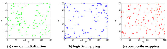
Figure 1.
One Hundred search agents generated by three methods.
3.2. Improved Random Searching Strategy
The random searching strategy enables whales to explore the search domain, and it plays a vital role in maintaining the diversity of whales. However, the whole swarm is attracted to a random whale individual during the search process. As a result of such strong randomness, the convergence rate and stability would be decreased. To address this, an improved random searching strategy that introduces the best individual as a reference target for whale position updating was proposed, and the blindness of the original approach was reduced to some extent. The model can be expressed by the following equation:
where rand3 and rand4 are random numbers inside [0,1], and K is a correction factor equals to 2. The main motivation that introduces random components was to enable WOA to show more random behaviors, which can make a noticeable difference to the exploration ability.
3.3. Modified Spiral Updating Position Strategy
The primary issue of the metaheuristic algorithms is that most of the searching agents prone to stagnation in local optimums owing to the defect in maintaining population diversity, and the conventional WOA algorithm is no exception. In the original spiral updating position strategy, the global optimal whale is taken as the target prey, and the other whales attempt to update their positions according to this optimal whale. However, if the present optimal whale traps into local optimal solution, the possibility of the whale swarm getting into local optimum will increase [28]. In the previous studies, the Lévy flight strategy has been widely adopted by metaheuristic algorithms because of its efficient global searchability. Therefore, we introduced the modified spiral updating position strategy based on Lévy flight to make up for the above drawback, and it will help the whales maintain diversity for longer and get rid of stagnation.
The random step generates by the Lévy flight strategy obeys the Lévy distribution. The levy distribution is a type of fat-tailed distribution, and its tail is wider than Gaussian distribution. Figure 2 shows 100 consecutive steps based on Lévy distribution and Gaussian distribution. It can be seen that Lévy flights can generate a large step occasionally, which means a stronger disturbance effect. However, with respect to Gaussian distribution, its steps are always small.
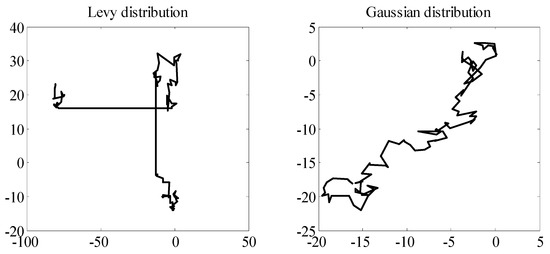
Figure 2.
Trajectories based on Lévy distribution and Gaussian distribution (starting from the origin).
The Lévy distribution is described as follows:
where s is the step size of Lévy flight, and it can also express as Levy(β). Generally, the algorithm proposed by Mantegna [47] was adopted to generate random steps, which have the same behavior as Levy flights. Thus, s can be calculated by the Equations (11) and (12):
where N denotes the Gaussian distribution, and the number of β is 1.5. The modified spiral updating position strategy is designed as follows: when the coefficient vector |A| ≥ 1, as aforementioned, it is in the exploration phase, whales are supposed to explore around themselves instead of the global optimal individual. The Lévy flight strategy was employed to generate a new movement when the position of the current whale individual is updated, and it performed the long-distance step occasionally so that the exploration ability was improved. The mathematical model can be expressed as follows:
When the coefficient vector |A| <1, the tendency of the searching process will turn to exploitation. Whales are expected to exploit within the encirclement centered on the current global optimal individual. This strategy also has a positive impact on achieving a better tradeoff between exploitation and exploration. It is defined by:
3.4. Modified Spiral Updating Position Strategy
In the original WOA algorithm, when a new position is beyond the search bounds, it usually replaces it by the bound. The proposed variant will change it by a random movement towards the search bound, which generally contributes to exploration. The new positions of whales are modified in accordance with the Equation (15).
where UB and LB are the upper bound and the lower bound, respectively; rand5 and rand6 are random numbers in [0,1].
3.5. Whole Framework for MSWOA
The main framework of the proposed MSWOA method is illustrated in Figure 3. First, the whale swarm was initialized by the chaotic initialization strategy. Thus, the initial whales could be evenly distributed in the search domain. Then, an improved random searching strategy and a modified spiral updating position strategy were introduced to make up the drawbacks of WOA and balance exploitation and exploration. Additionally, the enhanced position revising mechanism was adopted to make the whale population further explore the search space and yields a better MSWOA.
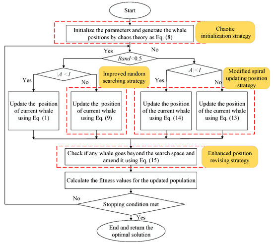
Figure 3.
Framework of the multi-strategy ensemble whale optimization algorithm (MSWOA).
4. Numerical Optimization Experiments
In this section, to testify the superiority of MSWOA, the proposed algorithm was compared with six well-designed algorithms base on nineteen benchmark functions. These algorithms include WOA [26], MFO [11], hybrid particle swarm optimization with spiral-shaped mechanism (HPSO-SSM) [48], GWO [10], PSO-GWO [49], and Lévy flight trajectory-based whale optimization algorithm (LWOA) [40]. The detailed information about benchmark functions, experimental settings, and simulation results are illustrated in the remaining part of this section.
4.1. Benchmark Functions
The parameter settings for the nineteen numerical benchmark functions, which are extensively used to verify the effectiveness of metaheuristics by many researchers [50,51,52], are presented in Table 1, where Dim, S, and fmin represent the dimension, the range of the solution domain, and the global optimum for each benchmark function, respectively. As shown in Table 1, there are three kinds of benchmark functions: The first group is seven unimodal benchmarks, which are usually utilized to test the exploitation ability. The second group includes six multimodal benchmarks, and Figure A1 presents the landscapes of four of the multimodal functions. It can be observed that there are many local optimal solutions near the global optimum, and the number of them will increase exponentially with dimension. The existence of these local optimal solutions increases the difficulty of finding the global optimal solution, which is a test for the exploration performance of the metaheuristics. The third group contains six fixed-dimension multimodal functions.

Table 1.
Benchmark functions.
4.2. Experimental Settings
All simulation experiments in this paper were performed on a PC independently, which had the following configuration: operating system, 64-bit Windows 10; CPU, Intel Core i5-8300 2.30 GHz, and simulation software, MATLAB R2012a. The specific information and parameter settings of the examined method are presented in Table 2. In this paper, 30 simulation experiments were carried out for each benchmark function with different dimensions, as listed in Table 1, and the average values (Mean), as well as the standard deviations (S.D.), are shown in Table 3. Meanwhile, all algorithms were sorted in accordance with its mean, and the rank results are presented in Table 3. Moreover, the population size and the maximum iteration numbers of all numerical optimization experiments were set to 40 and 500, respectively.
Table 2.
Parameters settings of examined algorithms.
Table 3.
Numerical optimization simulation results of WOA, MFO, HPSO-SSM, GWO, PSO-GWO, LWOA, and MSWOA.
4.3. Simulation Results Analysis
In this subsection, comparative numerical optimization experiments were conducted among the WOA [26], MFO [11], HPSO-SSM [48], GWO [10], PSO-GWO [49], LWOA [40], and MSWOA. Table 3 presents the mean and S.D. of the algorithms. Moreover, from Figure 4, Figure 5, Figure 6, Figure 7, Figure 8, Figure 9, Figure 10, Figure 11, Figure 12 and Figure 13, we can see the convergence curves for these seven metaheuristic swarm optimization algorithms.
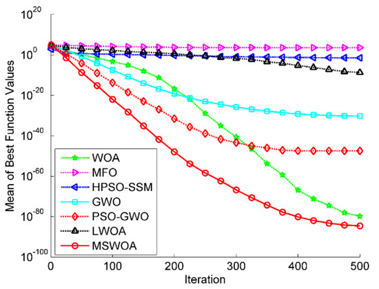
Figure 4.
Optimization results for F1 (Dim = 30).
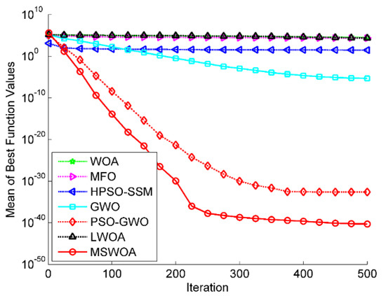
Figure 5.
Optimization results for F3 (Dim = 30).
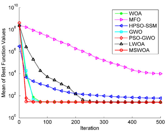
Figure 6.
Optimization results for F5 (Dim = 30).
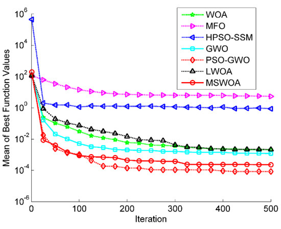
Figure 7.
Optimization results for F7 (Dim = 30).
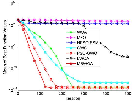
Figure 8.
Optimization results for F10 (Dim = 30).
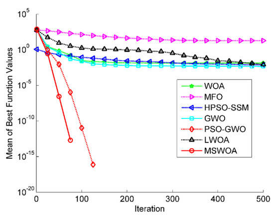
Figure 9.
Optimization results for F11 (Dim = 30).
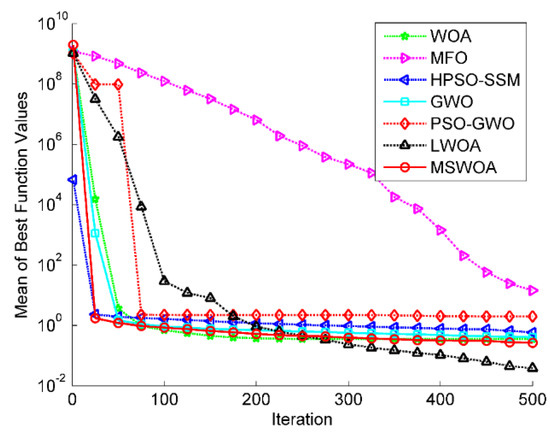
Figure 10.
Optimization results for F13 (Dim = 30).
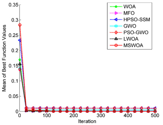
Figure 11.
Optimization results for F15 (Dim = 4).
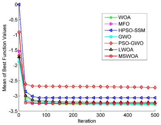
Figure 12.
Optimization results for F18 (Dim = 6).
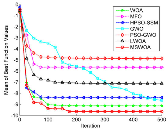
Figure 13.
Optimization results for F19 (Dim = 4).
4.3.1. Unimodal Function (F1–F7)
From Table 3, it can be indicated that the MSWOA method obtained a better performance compared with the other six optimization algorithms for most unimodal functions (F1, F2, F3, F4, and F5). Particularly, for functions F3 and F4, the average value and the standard deviation of MSWOA were significantly improved when compared with the standard WOA. This finding supports that the modified spiral updating position strategy was beneficial for MSWOA to balance the exploitation and exploration process, which cause the algorithm to have better search performance. In addition, LWOA showed strong competitiveness on function F6, and MSWOA did not perform as well as LWOA in this function but better than the standard WOA. Note that both MSWOA and LWOA adopted Lévy flight in designing their search mechanism. Regarding function F7, the PSO-GWO could achieved the best value, while MSWOA came in second place.
Figure 4, Figure 5, Figure 6 and Figure 7 illustrate the convergence curves of the average values of 30 runs for part of the unimodal benchmark functions (F1, F3, F5, and F7). Figure 4 shows that the MSWOA algorithm had the best search accuracy and the fastest convergence speed. Figure 5 indicates that MSWOA overtook the other six algorithms in terms of search results and convergence rate, while PSO-GWO ranked second. Figure 6 demonstrates that WOA, GWO, PSO-GWO, LWOA, and MSWOA had very close search accuracy, but the convergence speed of the proposed MSWOA was super to that of the other four algorithms. From Figure 7, it can be seen that MSWOA converged faster in the initial stage of the searching process, yet PSO-GWO obtained slightly higher search precision in the latter period.
4.3.2. Multimodal Functions (F8–F13):
As for the multimodal functions, several observations can be obtained based on Table 3: MSWOA cold locate the theoretically global optimum for functions F9 and F11. As a result of integrating the improved random searching strategy, as well as the enhanced position updating strategy, the exploration ability of MSWOA was strengthened. In addition, MSWOA outperformed the other six optimization methods on function F10, and its mean value had slight advantages when compared with WOA and PSO-GWO. On function F12 and F13, LWOA gained the best results, while the proposed MSWOA also exhibited strong competitiveness on these two multimodal functions. Moreover, WOA, LWOA, and MSWOA achieved similar mean values on function F8, which were better than the results of the other metaheuristics, but LWOA stood out among those three algorithms.
Figure 8, Figure 9 and Figure 10 are the convergence curves of partial multimodal functions (F10, F11, and F13). As shown in Figure 8, the MSWOA obtained a faster convergence speed and better search accuracy, and the WOA and PSO-GWO also displayed outstanding optimization results. Figure 9 demonstrates that MSWOA and PSO-GWO outperformed other methods as both of them could reach the global optimal value, but the convergence rate of MSWOA was higher. Figure 10 illustrates that all the tested algorithms, except MFO, obtained very close performances in the early stage; however, LWOA showed a promising final search accuracy.
4.3.3. Fixed-Dimension Multimodal Functions (F14–F19):
MSWOA generally overtook the other six algorithms. More precisely, MSWOA could nearly reach the best solution on functions F15, F16, and F19, and it also exhibited great advantages on stability. With respect to function F14, LWOA was superior to the other competitors. On function F17, MFO, HPSO-SSM, GWO, and MSWOA showed little difference in search accuracy, but HPSO-SSM was more stable. In addition, GWO got a high-quality mean solution on function F18.
Figure 11, Figure 12 and Figure 13 display the convergence graphs of three selected fixed-dimension multimodal functions (F15, F18, and F19). From Figure 11, we can see that the search results of all the algorithms were roughly the same. However, MSWOA owned the fastest convergence speed. Figure 12 presents that GWO had a better performance in search accuracy and convergence rate in the final stage. The plot in Figure 13 reveals that MSWOA possessed excellent capability in jumping out of the local optimums and converged towards the global optimum closely and quickly, while MFO and PSO-GWO reached the stagnation state prematurely, which led to poor search results.
Therefore, from the above descriptions and discussions of the simulation results of numerical optimization experiments, it can be seen that compared with other six SI algorithms, the proposed MSWOA method had better optimization accuracy and convergence speed for the majority of the nineteen classical benchmark problems, which indicates that the proposed strategies are practical and successful.
To further testify the effectiveness of the proposed variant, we applied MSWOA to analog circuits fault diagnosis, and the detailed information is presented in the next section.
5. Application of MSWOA in Fault Diagnosis of Analog Circuits
In this section, we utilized the Multisim14 software to simulate two well-known filter circuits, namely the Sallen–Key band pass filter circuit and the four-op-amp biquad high-pass filter circuit. For a start, we set the maximum deviation of components to be 40% for the soft faults. In each experiment, only one component was selected as the fault component at a time, and the parameters of other components were within the tolerance. Then, the Monte Carlo simulation analysis was conducted on each state of the test circuit. We extracted the features using a wavelet packet and then randomly divided those data into the training set and testing set. After that, the kernel parameter γ and the penalty parameter C of SVM were optimized by the proposed MSWOA method, while the diagnosis accuracy was defined as the fitness function of the MSWOA during the optimization process. Finally, we applied the trained SVM to the fault diagnosis of analog circuits.
We conducted a total of two sets of diagnosis experiments in this literature. Two different optimization methods, namely, PSO and WOA, were compared with the proposed MSWOA in each group of tests. The overall process of fault diagnosis of analog circuits based on SVM and MSWOA is illustrated in Figure 14.
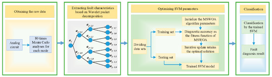
Figure 14.
The overall process of analog circuits fault diagnosis.
5.1. Fault Diagnosis of Sallen–Key Bandpass Filter Circuit
5.1.1. Simulation Settings
The Sallen–Key bandpass filter circuit is presented in Figure 15. Parameters of the circuit were set as follows: the resistor tolerance was rated to 5%, and the capacitance tolerance value was 10%. We applied a sinusoidal excitation signal to the circuit (amplitude 5 Vrms, period 10 kHz), and the voltage signals of the output node were collected.
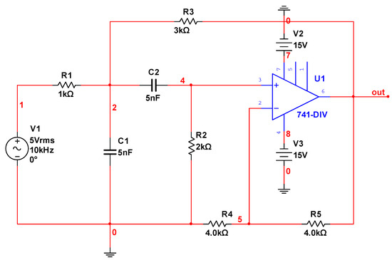
Figure 15.
Sallen–Key bandpass filter circuit.
As mention above, the maximum fault deviation rate was 40%, and the parameter settings of different fault categories are exhibited in Table 4, where ↑ represents the actual value was higher than the normal state, and ↓ represents the actual value was lower than the normal state. Table 4 indicates that the Sallen–Key band pass filter circuit had nine kinds of different running states, including one normal state and eight soft fault sates.
Table 4.
Fault types of the Sallen–Key bandpass filter circuit.
5.1.2. Feature Extraction
Feature extraction is a key step for many pattern recognition problems. In this paper, we used wavelet packet to extract features from the raw data sampled from the output node of the circuits. Part of the normalized fault features are shown in Figure 16. A total of eighty sets of data were gathered for each state. We randomly selected half of them as the training set, and the others as the testing set.
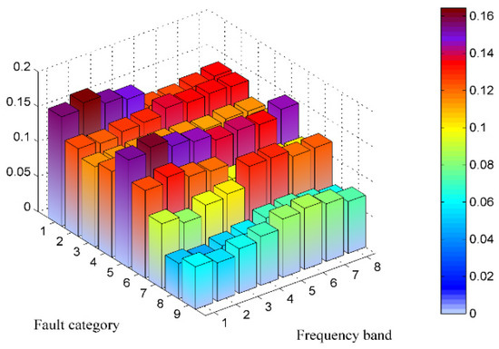
Figure 16.
Normalized fault features.
5.1.3. Experimental Results and Analyses
In this subsection, MSWOA was compared with two other SI algorithms (PSO and WOA) by optimizing the SVM parameters for fault diagnosis. These three algorithms adopted the same initialization parameters in the experiments: The population size and the maximum number of iterations were set to 20 and 100, respectively. For a fair comparison, each of the three algorithms was executed 20 times independently to eliminate the contingency of one experimental result. The statistical results are demonstrated in Figure 17, where the B.V., W.V., and A.V. mean the best value, the worst value, and the average value of the 20 experimental results, respectively.
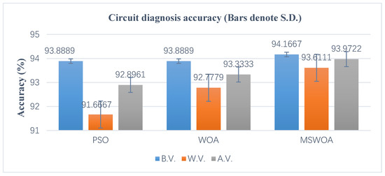
Figure 17.
Diagnosis results of the Sallen–Key band pass filter circuit.
As we can see from Figure 17, due to the strong searchability of MSWOA, the optimal value of the diagnosis result of SVM optimized by MSWOA was the greatest. Regarding the worst value, the result obtained by the MSWOA-SVM method was increased about 1.94% and 0.83% compared to that of PSO-SVM and WOA-SVM. And when it comes to the average value, the result of MSWOA-SVM was 1.07% and 0.64% higher than that of PSO-SVM and WOA-SVM, which indicates that the MSWOA algorithm improved its capacity of escaping the local optimal solution. In addition, Figure A2 presents the box plots, which include the median value, the upper and lower edges, and the 3/4 and 1/4 values in 20 results. It can be observed that the whole distribution of MSWOA was more concentrated than its competitors, which means MSWOA has stronger stability and robustness.
Figure 18 shows the diagnostic accuracy curves of SVM optimized by PSO, WOA, and MSWOA, respectively. In each of those three figures, the mean fitness curve and the best fitness curve were obtained by the whole population in one optimization process (100 iterations). From those figures, we can conclude that the SVM optimized by the proposed MSWOA had the best performances in accuracy and speed.
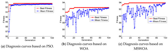
Figure 18.
Fault diagnosis accuracy curves of the three methods optimized support vector machine (SVM).
5.2. Fault Diagnosis of Four-Op-Amp Biquad High-Pass Filter Circuit
5.2.1. Simulation Settings
The second group of fault diagnosis experiments was conducted on the four-op-amp biquad high-pass filter circuit, as shown in Figure 19. The parameters of which were set as follows: the value of resistor tolerance in the circuit was 5%, while the capacitance tolerance was rated to 10%. In addition, we applied a sinusoidal excitation signal (amplitude 10 Vrms, frequency 2 kHz) to this circuit, and collect the voltage signal outputs from the out node.
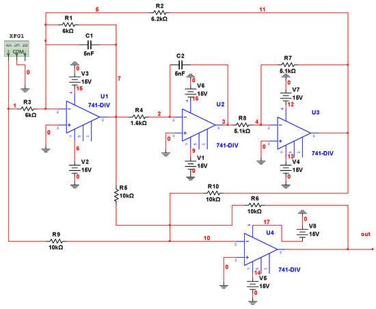
Figure 19.
Four-op-amp biquad high-pass filter circuit.
The maximum fault deviation rate was set to 40%, and the parameter settings of different fault types are exhibited in Table 5, where ↑ represents the actual value is higher than the normal state, and ↓ represents the actual value is lower than the normal state. It can be concluded from Table 5, there were seven kinds of different running states, including one normal state and six soft fault sates, for the four-op-amp biquad high-pass filter circuit.
Table 5.
Fault types of four-op-amp biquad high-pass filter circuit.
5.2.2. Experimental Results and Analyses
Similar to the first group of analog circuit fault diagnosis experiment described in the previous subsection, in this part, the MSWOA algorithm was compared with PSO and WOA by optimizing the SVM parameters for fault diagnosis. The initialization parameters settings for the three metaheuristic optimization algorithms were identical to the first group, i.e., the swarm size was 20, and the maximum steps of iterations were 100. To avoid the contingency of one experimental result, we performed 20 executions of each algorithm, and the statistics are presented in Figure 20, where the B.V., W.V., and A.V. mean the best value, the worst value, and the average value of the twenty experimental results, respectively.
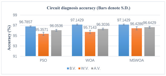
Figure 20.
Diagnosis results of four-op-amp biquad high-pass filter circuit.
As shown in Figure 20, the proposed MSWOA method did better than the other two algorithms, which means that the proposed strategies effectively facilitate the performances of the original WOA algorithm. Besides, Figure A3 illustrates the box plots achieved by the 20 diagnosis results. It can be noticed that the MSWOA method obtained a more concentrated distribution, which indicates a lower standard deviation. Additionally, the red curves and the blue curves shown in Figure 21 are the best fitness values and the mean fitness values obtained by the whole population in one optimization process (100 iterations) of PSO, WOA, and MSWOA, respectively. From this figure, we can conclude that the classifiers optimized by the proposed MSWOA and WOA had better performances in accuracy. In general, SVM optimized by the MSWOA algorithm was more practical and efficient in circuit fault diagnosis.
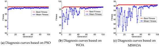
Figure 21.
Fault diagnosis accuracy curves of the three methods optimized SVM.
6. Conclusions
Faced with complex optimization problems, the original WOA algorithm may drive the search to premature convergence or be stuck at the local optimal solutions, etc. To overcome those disadvantages, a multi-strategy ensemble whale optimization algorithm (MSWOA) was developed in this paper. The proposed MSWOA first adopted the chaotic initialization strategy so that the whale swarm could be evenly distributed in the search area. Then, two strategies of the conventional WOA was modified to facilitate its search performance. More precisely, by introducing the best search agent as a reference target, the random searching strategy was enhanced to reduce blindness and accelerate the convergence during optimization. Furthermore, the spiral updating position strategy was improved by the Levy flight, which has a high ability to balance exploration and exploitation. Finally, the enhanced position revising mechanism was designed to strengthen exploration ability further and yields a better MSWOA.
A large number of comparative experiments were conducted to validate the effectiveness of the MSWOA algorithm. For a start, we performed extensive numerical optimization simulation experiments based on nineteen classical benchmark problems, which were extensively used to test the performance of metaheuristics. Moreover, MSWOA was thoroughly compared with six well-established optimization methods. Comparison results indicated that the proposed MSWOA could achieve good results for the majority of the nineteen benchmark problems. Additionally, to further testify the performances of the MSWOA algorithm, we applied the MSWOA to the fault diagnosis of analog circuits. Empirical studies indicated that the diagnostic accuracy of the SVM optimized by the proposed MSWOA was the highest, which reflects that MSWOA possesses excellent practicability in the circuit fault diagnosis field. Therefore, the proposed MSWOA can be considered as a novel and efficient tool for addressing the numerical optimization problems and analog circuit fault diagnosis tasks.
However, for a few fixed-dimension multimodal functions, MSWOA had no obvious superiorities compared with other algorithms. Therefore, how to facilitate the MSWOA accuracy and speed for fixed-dimension multimodal functions still deserves further study.
Author Contributions
Conceptualization, X.Y. and Z.M.; Investigation, Z.M. and Z.Y.; Methodology, X.Y., Z.M. and Z.L.; Software, Z.M. and Z.L.; Supervision, X.Y. and F.Z.; Validation, Z.L. and Z.Y.; Writing—original draft, X.Y. and Z.M. All authors have read and agreed to the published version of the manuscript.
Funding
This work is supported by the National Natural Science Foundation of China (Grant No. 61803227, 61973184, 61773242, 61603214), The National Key R & D Program of China (Grant No.2017YFB1302400), Key Research and Development Program of Shandong Province (Grant No. 2018GGX101039), Independent Innovation Foundation of Shandong University (Grant No. 2082018ZQXM005).
Acknowledgments
We would like to thank the editors and the anonymous reviewers for their insightful comments and constructive suggestions.
Conflicts of Interest
The authors declare that there is no conflict of interest regarding the publication of this paper.
Appendix A

Figure A1.
2-Dimensional forms of the multimodal functions.


Figure A2.
Box plots of fault diagnosis results of the Sallen–Key band pass filter circuit.


Figure A3.
Box plots of fault diagnosis results of four-op-amp biquad high-pass filter circuit.

References
- Elaziz, M.A.; Mirjalili, S.A. Hyper-heuristic for improving the initial population of whale optimization algorithm. Knowl. Based Syst. 2019, 172, 42–63. [Google Scholar] [CrossRef]
- Castillo-Martinez, A.; Almagro, J.R.; Gutierrez-Escolar, A.; Corte, A.D.; Castillo-Sequera, J.L.; Gómez-Pulido, J.M.; Gutiérrez-Martínez, J.M. Particle swarm optimization for outdoor lighting design. Energies 2017, 10, 141. [Google Scholar] [CrossRef]
- Tu, Q.; Chen, X.; Liu, X. Multi-strategy ensemble grey wolf optimizer and its application to feature selection. Appl. Soft Comput. 2019, 76, 16–30. [Google Scholar] [CrossRef]
- Wang, G.; Cai, X.; Cui, Z. High performance computing for cyber physical social systems by using evolutionary multi-objective optimization algorithm. IEEE Trans. Emerg. Top. Comput. 2020, 8, 20–30. [Google Scholar] [CrossRef]
- Li, X.; Shao, Z.; Qian, J. An optimizing method based on autonomous animate: Fish-swarm algorithm. Syst. Eng. Theory Pract. 2002, 11, 32–38. [Google Scholar]
- Basturk, B.; Karaboga, D. An artificial bee colony (ABC) algorithm for numeric function optimization. In Proceedings of the IEEE Swarm Intelligence Symposium, Indianapolis, IN, USA, 12–14 May 2006; pp. 181–184. [Google Scholar]
- Yang, X.S. Firefly algorithms for multimodal optimization. In Proceedings of the International Symposium on Stochastic Algorithms, Sapporo, Japan, 26–28 October 2009; pp. 169–178. [Google Scholar]
- Gandomi, A.H.; Alavi, A.H. Krill herd: A new bio-inspired optimization algorithm. Commun. Nonlinear Sci. Numer. Simul. 2012, 17, 4831–4845. [Google Scholar] [CrossRef]
- Das, K.N.; Singh, T.K. Drosophila food-search optimization. Appl. Math. Comput. 2014, 231, 566–580. [Google Scholar] [CrossRef]
- Mirjalili, S.; Mirjalili, S.M.; Lewis, A. Grey wolf optimizer. Adv. Eng. Softw. 2014, 69, 46–61. [Google Scholar] [CrossRef]
- Mirjalili, S. Moth-flame optimization algorithm: A novel nature-inspired heuristic paradigm. Know. Based Syst. 2015, 89, 228–249. [Google Scholar] [CrossRef]
- Zhang, C.; He, Y.; Yuan, L. Analog circuit incipient fault diagnosis method using DBN based features extraction. IEEE Access 2018, 6, 23053–23064. [Google Scholar] [CrossRef]
- Binu, D.; Kariyappa, B.S. RideNN: A New Rider Optimization Algorithm-Based Neural Network for Fault Diagnosis in Analog Circuits. IEEE Trans. Instrum. Meas. 2018, 68, 1–25. [Google Scholar] [CrossRef]
- Hu, X.; Moura, S.; Murgovski, N. Integrated optimization of battery sizing, charging, and power management in plug-in hybrid electric vehicles. IEEE Trans. Control Syst. Technol. 2015, 24, 1036–1043. [Google Scholar] [CrossRef]
- Arias-Guzman, S.; Ruiz-Guzmán, O.; Garcia-Arías, L. Analysis of voltage sag severity case study in an industrial circuit. IEEE Trans. Ind. Appl. 2016, 53, 15–21. [Google Scholar] [CrossRef]
- Zhang, A.; Chen, C.; Jiang, B. Analog circuit fault diagnosis based UCISVM. Neurocomputing 2016, 173, 1752–1760. [Google Scholar] [CrossRef]
- Vasan, A.; Pecht, M. Electronic circuit health estimation through kernel learning. IEEE Trans. Ind. Electron. 2017, 65, 1585–1594. [Google Scholar] [CrossRef]
- Chen, P.; Yuan, L.; He, Y. An improved SVM classifier based on double chains quantum genetic algorithm and its application in analogue circuit diagnosis. Neurocomputing 2016, 211, 202–211. [Google Scholar] [CrossRef]
- Wang, T.; Qi, J.; Xu, H. Fault diagnosis method based on FFT-RPCA-SVM for cascaded-multilevel inverter. ISA Trans. 2016, 60, 156–163. [Google Scholar] [CrossRef]
- Long, B.; Xian, W.; Li, M. Improved diagnostics for the incipient faults in analog circuits using LSSVM based on PSO algorithm with Mahalanobis distance. Neurocomputing 2014, 133, 237–248. [Google Scholar] [CrossRef]
- Wei, J.; Zhang, R.; Yu, Z. A BPSO-SVM algorithm based on memory renewal and enhanced mutation mechanisms for feature selection. Appl. Soft Comput. 2017, 58, 176–192. [Google Scholar] [CrossRef]
- Lu, J.; Liao, X.; Li, S. An Effective ABC-SVM Approach for surface roughness prediction in manufacturing processes. Complexity 2019, 3094670, 1–13. [Google Scholar] [CrossRef]
- Li, K.; Cheng, G.; Sun, X. A nonlinear flux linkage model for bearingless induction motor based on GWO-LSSVM. IEEE Access 2019, 7, 36558–36567. [Google Scholar] [CrossRef]
- Li, C.; An, X.; Li, R. A chaos embedded GSA-SVM hybrid system for classification. Neural Comput. Appl. 2015, 26, 713–721. [Google Scholar] [CrossRef]
- Jiang, M.; Luo, J.; Jiang, D. A cuckoo search-support vector machine model for predicting dynamic measurement errors of sensors. IEEE Access 2016, 4, 5030–5037. [Google Scholar] [CrossRef]
- Mirjalili, S.; Lewis, A. The whale optimization algorithm. Adv. Eng. Softw. 2016, 95, 51–67. [Google Scholar] [CrossRef]
- Gharehchopogh, F.; Gholizadeh, H. A comprehensive survey: Whale Optimization Algorithm and its applications. Swarm Evol. Comput. 2019, 48, 1–24. [Google Scholar] [CrossRef]
- Zhang, Q.; Liu, L. Whale optimization algorithm based on lamarckian learning for global optimization problems. IEEE Access 2019, 7, 36642–36666. [Google Scholar] [CrossRef]
- Mehne, H.; Mirjalili, S. A parallel numerical method for solving optimal control problems based on whale optimization algorithm. Knowl. Based Syst. 2018, 151, 114–123. [Google Scholar] [CrossRef]
- Mafarja, M.M.; Mirjalili, S. Hybrid Whale Optimization Algorithm with simulated annealing for feature selection. Neurocomputing 2017, 260, 302–312. [Google Scholar] [CrossRef]
- Mafarja, M.; Mirjalili, S. Whale optimization approaches for wrapper feature selection. Appl. Soft Comput. 2018, 62, 441–453. [Google Scholar] [CrossRef]
- Aziz, M.A.; Ewees, A.A.; Hassanien, A.E. Whale optimization algorithm and moth-flame optimization for multilevel thresholding image segmentation. Expert Syst. Appl. 2017, 83, 242–256. [Google Scholar] [CrossRef]
- Medani, K.; Sayah, S.; Bekrar, A. Whale optimization algorithm based optimal reactive power dispatch: A case study of the Algerian power system. Electr. Power Syst. Res. 2018, 163, 696–705. [Google Scholar] [CrossRef]
- Xiong, G.; Zhang, J.; Yuan, X. Parameter extraction of solar photovoltaic models by means of a hybrid differential evolution with whale optimization algorithm. Solar Energy 2018, 176, 742–761. [Google Scholar] [CrossRef]
- Petrović, M.; Miljković, Z.; Jokić, A. A novel methodology for optimal single mobile robot scheduling using whale optimization algorithm. Appl. Soft Comput. 2019, 81, 1–25. [Google Scholar] [CrossRef]
- Peng, H.; Wen, W.; Tseng, M.; Li, L. Joint optimization method for task scheduling time and energy consumption in mobile cloud computing environment. Appl. Soft Comput. 2019, 80, 534–545. [Google Scholar] [CrossRef]
- Li, L.; Sun, J.; Tseng, M.; Li, Z. Extreme learning machine optimized by whale optimization algorithm using insulated gate bipolar transistor module aging degree evaluation. Expert Syst. Appl. 2019, 127, 58–67. [Google Scholar] [CrossRef]
- Chen, H.; Xu, Y.; Wang, M. A balanced whale optimization algorithm for constrained engineering design problems. Appl. Math. Model. 2019, 71, 45–59. [Google Scholar] [CrossRef]
- Li, Y.; Han, T.; Zhao, H. An Adaptive whale optimization algorithm using Gaussian distribution strategies and its application in heterogeneous UCAVs task allocation. IEEE Access 2019, 7, 110138–110158. [Google Scholar] [CrossRef]
- Ling, Y.; Zhou, Y.; Luo, Q. Lévy flight trajectory-based whale optimization algorithm for global optimization. IEEE Access 2017, 5, 6168–6186. [Google Scholar] [CrossRef]
- Sun, Y.; Wang, X.; Chen, Y. A modified whale optimization algorithm for large-scale global optimization problems. Expert Syst. Appl. 2018, 114, 563–577. [Google Scholar] [CrossRef]
- Yousri, D.; Allam, D.; Eteiba, M. Chaotic whale optimizer variants for parameters estimation of the chaotic behavior in Permanent Magnet Synchronous Motor. Appl. Soft Comput. 2019, 74, 479–503. [Google Scholar] [CrossRef]
- Abdel-Basset, M.; Manogaran, G.; El-Shahat, D. Integrating the whale algorithm with Tabu search for quadratic assignment problem: A new approach for locating hospital departments. Appl. Soft Comput. 2018, 73, 530–546. [Google Scholar] [CrossRef]
- Tian, D.; Zhao, X.; Shi, Z. Chaotic particle swarm optimization with sigmoid-based acceleration coefficients for numerical function optimization. Swarm Evol. Comput. 2019, 51, 1–16. [Google Scholar] [CrossRef]
- García-Ródenas, R.; Linares, L.; López-Gómez, J. A Memetic Chaotic Gravitational Search Algorithm for unconstrained global optimization problems. Appl. Soft Comput. 2019, 79, 14–29. [Google Scholar] [CrossRef]
- Rizk-Allah, R.; Hassanien, A.; Bhattacharyya, S. Chaotic crow search algorithm for fractional optimization problems. Appl. Soft Comput. 2018, 71, 1161–1175. [Google Scholar] [CrossRef]
- Mantegna, R.N. Fast. Accurate algorithm for numerical simulation of Levy stable stochastic processes. Phys. Rev. E 1994, 49, 4677–4683. [Google Scholar] [CrossRef]
- Chen, K.; Zhou, F.; Yuan, X. Hybrid particle swarm optimization with spiral-shaped mechanism for feature selection. Expert Syst. Appl. 2019, 128, 140–156. [Google Scholar] [CrossRef]
- Teng, Z.; Lv, J.; Guo, L. An improved hybrid grey wolf optimization algorithm. Soft Comput. 2019, 23, 6617–6631. [Google Scholar] [CrossRef]
- Al-Betar, M.; Awadallah, M.; Faris, H. Natural selection methods for grey wolf optimizer. Expert Syst. Appl. 2018, 113, 481–498. [Google Scholar] [CrossRef]
- Lu, C.; Gao, L.; Yi, J. Grey wolf optimizer with cellular topological structure. Expert Syst. Appl. 2018, 107, 89–114. [Google Scholar] [CrossRef]
- Liu, X.; Tian, Y.; Lei, X. An improved self-adaptive grey wolf optimizer for the daily optimal operation of cascade pumping stations. Appl. Soft Comput. 2019, 75, 473–493. [Google Scholar] [CrossRef]


© 2020 by the authors. Licensee MDPI, Basel, Switzerland. This article is an open access article distributed under the terms and conditions of the Creative Commons Attribution (CC BY) license (http://creativecommons.org/licenses/by/4.0/).