1. Introduction
The actual application of structural analysis deals with complex constructions subjected to randomly variable loads. Generally, the load intensity bounds are prescribed by standards and authorities and are evaluated by starting from probabilistic and statistical considerations. It is almost impossible, in practical cases, to know actual load history and their distribution all over the structure, considering that only their intensity range is estimated.
Under these hypotheses, evaluating structural safety is a matter of overall consideration rather than the specific pointwise calculation of the response.
Under the above-quoted circumstances, the main strategy for structural safety assessment is the calculation of load collapse limit, both under proportionally and randomly variable cases [
1,
2].
The former case cited above concerns the evaluation of the usual collapse limit, whereas the latter, besides the collapse limit, requires the calculation of the shakedown limit. Under variable loads, whenever the load reaches the collapse limit, the structure can undergo a sudden collapse. Moreover, it is possible that although at no time collapse occurs, the structure is invested by plastic deformation that during load path increases in time. Now three phenomena can present on the structure: first, the displacement increases in time indefinitely and the structure fails at the end for excessive strain (ratcheting); second, the plastic strain changes sign indefinitely during load path hence, although no excessive displacement occurs the structure fails for plastic fatigue; third, the plastic strain produces self-equilibrated stress that prevents the structure from accumulating further plastic strain, and it starts to definitely behave as elastic. This latter case is called shakedown. The shakedown limit is the load level that the structure shakes down, whilst over it, the structure suffers ratcheting or plastic fatigue [
2]. In this situation, some specification should be done about the velocity of the phenomenon to distinguish between elastic and plastic shakedown propagation, but here only statics will be considered [
3,
4,
5].
Generally, the knowledge of the structural limit load is pursued using step by step or limit analyses. This latter method is based on the two approaches coming from the upper bound and of the lower bound theorems [
1,
6]. These theorems are based on kinematic and static approaches, respectively. The first is aimed at calculating the limit load as the maximum among any statically admissible loads and the second as the minimum among any kinematically admissible loads. Both calculations are independent of the actual load histories, and although this is useful in the real-life analysis where the loads are known only in terms of their intensity bounds, it constitutes a limitation for the use of the method since it cannot evaluate the dissipation during ultra-elastic deformation. It is possible, therefore, that the permanent deformation, required for the ultra-elastic load path to develop, attains its limit before the collapse. Such an eventuality causes the limit analysis to fail since the collapse occurs before the complete permanent deformation develops. This happens at an actual load level lower than the theoretical limit.
This disadvantage is only apparently overcome by the step-by-step analysis since this approach is linked to the knowledge of the actual load history and gives results that cannot be generalized.
In the modern application of structural engineering, the numerical formulation of the limit analysis allows the application of the methods to a wide range of structures. In particular, the finite element method (FEM) has wide application to two- and three-dimensional structures. In [
7,
8], shakedown analysis for elastic-perfect plastic frames is discussed, and an incremental-iterative solution is proposed. A general procedure dealing with finite element application for lower bound determination of collapse and ratcheting load is in [
9]. As stated before, one of the most important weaknesses of limit analysis is that no direct information is given by the theoretical fundamentals of the analysis about the dissipation during the deformation process. It must be stressed that one of the hypotheses at the basis of the limit design is that the strain can develop completely until the load reaches its limit, namely, the permanent strain must be limited within the admissible amount. Only the knowledge of the load history allows precisely evaluating the amount of dissipated energy until the limit is attained.
Hence, many works estimate the ultimate dissipation and displacements during plastic loading of structures at the incoming plastic collapse or to ratcheting [
10,
11,
12], starting from Ponter that proposes a limit on the dissipated work and residual displacement [
13,
14]. In the present work, a procedure has been presented through Melan’s theorem [
6] of the shakedown. The procedure has used the “strain-based residual” stress that constitutes a basis of the vector space of the self-equilibrated stresses. Such residual stress fulfills Melan’s lower bound theorem and has been used to calculate upper bounds of the global and local dissipated work at the ultimate load level and pointwise permanent strain as well.
The method has proposed, in the framework of discontinuous FEM, a linear optimization strategy that gives an upper bound of local dissipation and, finally, an estimate of local permanent displacement. In the paper, the numerical procedure has been applied to an academic example of a one-dimensional structure. Concerning a one-dimensional example, the numerical procedure was also compared to the experimental results obtained by the authors in previous work [
15]. The experiment has concerned an aluminum beam over three supports, loaded by randomly variable one-point forces applied at the middle of each span. The structure has been loaded up to the shakedown limit and subsequently to ratcheting. The displacement has been measured during the loading process. The experimental results have been compared with the calculated ones, and a good agreement has been shown between theoretical and experimental approaches.
2. Fundamentals of Limit Analysis
A structure collapses if the dissipation due to permanent deformation increases in time indefinitely. The dissipation increment can be produced by proportionally increasing loads, hence, proper proportional collapse occurs. With no difference, the dissipation can increase in time alternating periods when no dissipation occurs and periods when dissipation gets further increase. In this latter case, it is possible that either the displacement becomes excessive for functionality and safety, or the total dissipation reaches a limit that produces the material failure. The first is the ratcheting phenomenon, the second the plastic fatigue rupture (also known as low cycle number fatigue) [
16].
To evaluate the load collapse multiplier, the static collapse theorem states that if under actual loads, there exists any equilibrated stress that definitely belongs to the elastic domain, the permanent strain rate vanishes whenever time increasing, hence collapse does not occur [
1]. In other words, the structure does stabilize, i.e., the structure behaves as to be elastic after that a certain amount of permanent strain has been accumulated. Moreover, a limiting equation exists that gives an upper bound of the dissipated energy until stabilization occurs [
14,
17].
The present work has described a numerical procedure that implemented the Melan theorem. For the sake of completeness, the Melan theorem has been reported hereafter briefly.
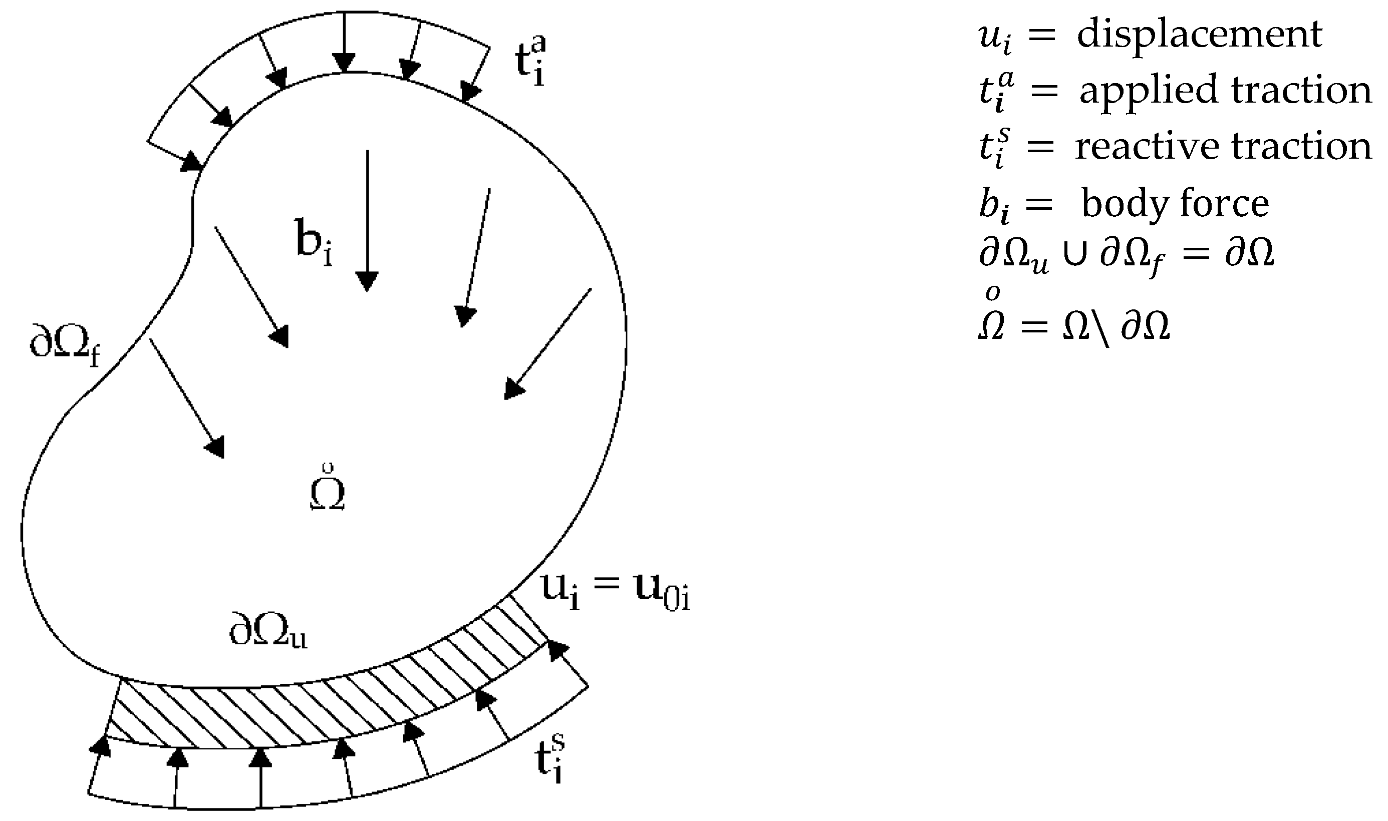
Let us consider a structure that occupies a domain
with the boundary
(
Figure 1). The structure is in equilibrium under prescribed body forces,
, in the interior of the solid,
, and prescribed tractions,
, on the part of the boundary
; both forces vary in time within the prescribed limit with absolutely random time law. On the part of the boundary,
, where the symbol \ denotes the complement of the manifold
with respect to
, the displacement is prescribed [
18]. Due to the applied loads and displacements, the solid presents the stress,
and the strain,
, in the interior and reactive tractions,
, on the boundary
. In the following, indicial notation is adopted hence a subscript ()
i have denoted the
ith component of a vector in the reference frame, two subscripts have referred to the two components of a second-order tensor and so on; moreover, subscripts following the comma indicate partial derivatives with respect to the coordinate directions.
Self-equilibrated stress,
, is a stress field that satisfies the homogeneous balance equations and the corresponding homogeneous natural boundary conditions on the loaded boundary
. Only on the constrained boundary
tractions can be non-null:
where in Equation (1),
are the components of the outward normal unit vector to
.
The material constituting the structure is elastic-perfectly plastic, so the stress–strain law is
where
is the fourth-order elastic tensor.
The permanent strain,
, results from the integration during the load process of the permanent strain rate,
, that is related to the stress through the constitutively associated flow rule:
where
is the compatibility condition on stress, equality holds for yielding,
is the gradient of the yield surface with respect to
and
is the plastic multiplier that accounts for the magnitude of the plastic strain rate,
.
During the loading process, the stress results by the superimposition of the one calculated on the structure supposed to be indefinitely elastic,
, and self-equilibrated stress,
, obtained by Equation (1), here called “eigenstress” [
19], can also be recognized to be the actual residual stress one finds in the structures, whether it is unloaded during the load path so that it can also be called “actual residual stress”:
The actual strain field results from the following additive decomposition that can be interpreted through the decomposition (4) yielding to the equation:
where
is the elastic compliance tensor, the inverse of
. Equation (5) has the following mechanical interpretation:
, is the sum of the strain in the structure supposed to be indefinitely elastic,
, the strain corresponding to the eigenstress,
and the permanent strain,
. The permanent strain
is the discontinuous part of the strain. It is possible to recognize the kinematical compatibility of the strain, namely:
is compatible since it is the elastic solution under the applied loads; the sum
is compatible as the strain
is the elastic response to the discontinuity
, acting as an applied dislocation, to ensure its compatibility [
2].
The stress
is self-equilibrated stress by definition. To verify the statement, the equilibrium equation of the interior points of the solid body is recalled:
By using Equations (4) and (5), the equilibrium of internal points become
The elastic stress is the stress in equilibrium in
, when the constitutive equation is assumed to be indefinitely elastic, subjected to the same loads than the actual structure. Consequently, the elastic stress,
, is in equilibrium with the applied forces so that the following equation holds:
Comparing Equation (7) with Equation (8), the following equation is obtained, confirming that the elastic-plastic stress is self-equilibrated in the interior of the structure.
Moreover, the self-equilibrated stress satisfies the homogeneous boundary condition on the free boundary, , of the structure. Finally, the equilibrium equation involving the stress reduces to Equation (1).
The above reasoning can be summarized as follows: the actual elastic–plastic stress solution, resulting from an applied body and boundary loads, differs from the pure elastic stress by self-equilibrated stress. This self-equilibrated stress is due to elastic strain
that results from the compatibility equation concerning the permanent discontinuous strain
acting as Volterra’s dislocation. Dislocations are the kinematical effect equivalent to discontinuities of strain within the structure. A dislocation causes stress in the absence of loads. The stress produced by dislocation is hence an eigenstress and satisfy Equations (1) and (10). The stress
, that depends on
, through Equation (9), emerges on the constrained boundary in terms of self-equilibrated traction,
.
3. Lower Bound Limit Analysis
The shakedown is the phenomenon where under randomly repeated loads, the structure undergoes elastic behavior definitely for increasing time. In other words, the permanent strain rate approaches zero for t→∞, hence the permanent strain is bounded in time. In the present formulation, the time is solely the measure of the evolution of the phenomenon, because of the rate of the quantities involved must be considered as their increment, no dynamics effects are considered.
The shakedown is ruled by Melan’s theorem. The theorem is formulated in term of self-equilibrated stress of the form .
The line of reasoning of Melan’s theorem is suitable as well for the application to the monotone load-induced collapse analysis.
In the following formulation the is obtained from the as the resulting stress from the application of the as Volterra’s dislocation.
It is possible to solve the elastic problem of the structure subjected by Volterra’s dislocation,
at a point
x and calculate, at any point
y, the resulting stress
. The linearity of the elastic problem allows writing the
in terms of the linear operator
. In numerical application a discrete approximation of the operator
can be obtained using the boundary integral equation method [
20]
Finally, the relationship between
and
can be written as follows:
The condition of shakedown is stated by Melan’s theorem in the following form: stabilization occurs under a load multiplier
k if and only if there exists a self-equilibrated stress
, time-independent eigenstress, such that:
at any time where
is the actual stress under the applied loads when the structure was supposed indefinitely elastic.
By considering Equation (11), Melan’s theorem can be rewritten in terms of permanent strain
such that
The optimization program that searches for the load limit multiplier,
sc, is summarized in
Program (14) is a constrained optimization program that can be solved using a standard linear programming routine, namely, the simplex method, if the constraints are a set of linear inequalities. This occurs when von Mises or Drucker–Prager limit-domains describe the material behavior.
The solution of the program (14) is the limit collapse multiplier that is either the proportional collapse multiplier, , or the shakedown limit, , provided the elastic stress corresponds to monotone or variable loads. Moreover, the program furnishes a set of permanent time-independent strain satisfying the theorem.
As a corollary of Melan’s theorem, see Koiter and Köning [
1,
16,
21], an upper bound on total dissipated energy until stabilization is obtained as a function of the elastic strain energy corresponding to Melan’s residual strain,
.
where the term on the left-hand side of Equation (15) is a lower bound of the total dissipation up to the load level, having the safety factor
with respect to the limit at the incoming collapse.
The inequality at the leftmost side of Equation (16) holds if the material of the structures follows von Mises or Drucker-Prager associate constitutive law. The integral on the third side of Equation (16) underestimates the case when the permanent strain reverses its sign and cancels. In the latter case, the time integration summed the work the stress did for increasing strain and that for the opposite strain. Conversely, the integral at the third side neglected this contribution.
Moreover, the right-hand side of Equation (15) is the elastic strain energy of Melan’s residuals,
Finally, in (15) the safety coefficient,
m, of the actual load multiplier for the considered collapse is introduced:
Equation (16) constitutes a constraint where the actual permanent strain
must satisfy during the loading process up to the load multiplier
. It is, then, possible to define a second optimization program by remembering Equation (11):
that can be used to calculate residual displacement upper-bound at a specific point,
x, of the structure. In Equation (19), the objective function can be any linear combination of the permanent strain; hence, any displacement can be calculated using (19) even if it is not a variable of the inequalities provided linear relationship holds between displacements and dislocations.
4. Numerical Example
The described method has been applied to structures made of one-dimensional beams. The beams are plane and are subjected to flexural loads. Shear effects are negligible so that only bending moment has been considered. The compatibility condition has reduced to the simple limitation of the bending moment, namely,
In Equation (20),
[
] represents the negative (positive) limit bending moment of the beam cross-section, respectively.
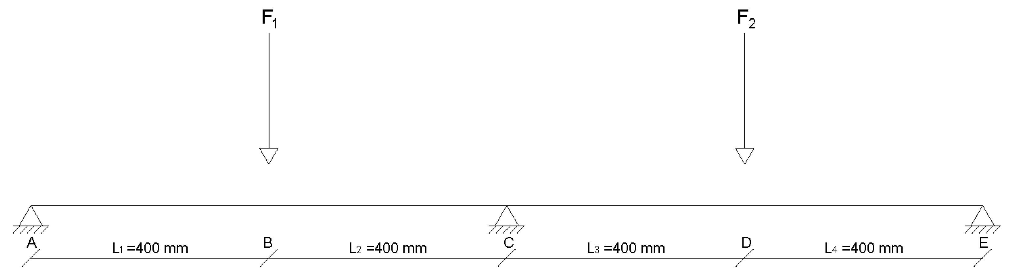
The results have been compared with the experimental ones presented in [
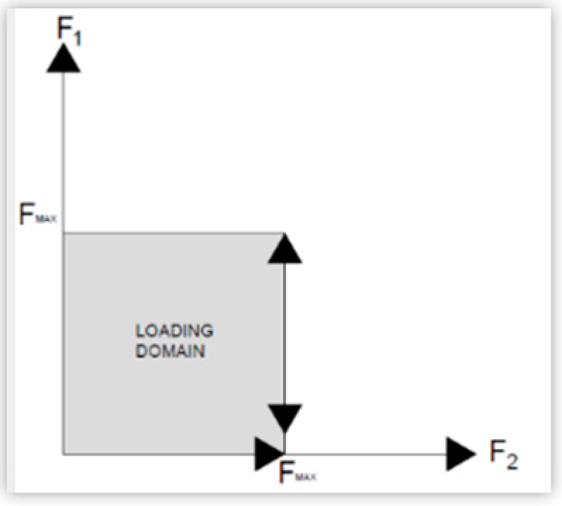
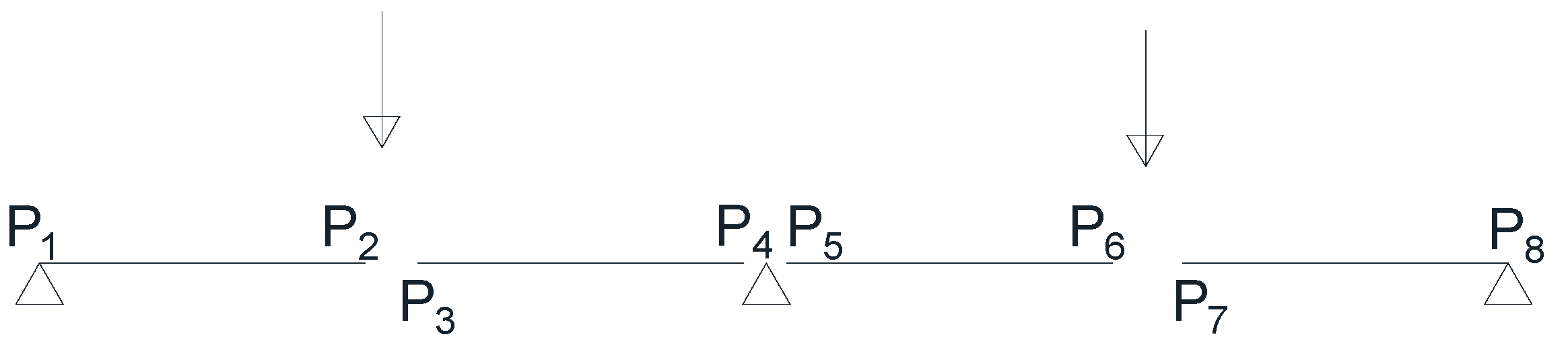
15]. The experimental set up has been briefly recalled in the following. The tested structure was an aluminum beam, over three supports. The supports were equally spaced; the beam was loaded by one-point forces applied at the middle of each span. The forces, F
1 and F
2 (see
Figure 2), have varied accordingly with the load program whose diagram has been drawn in
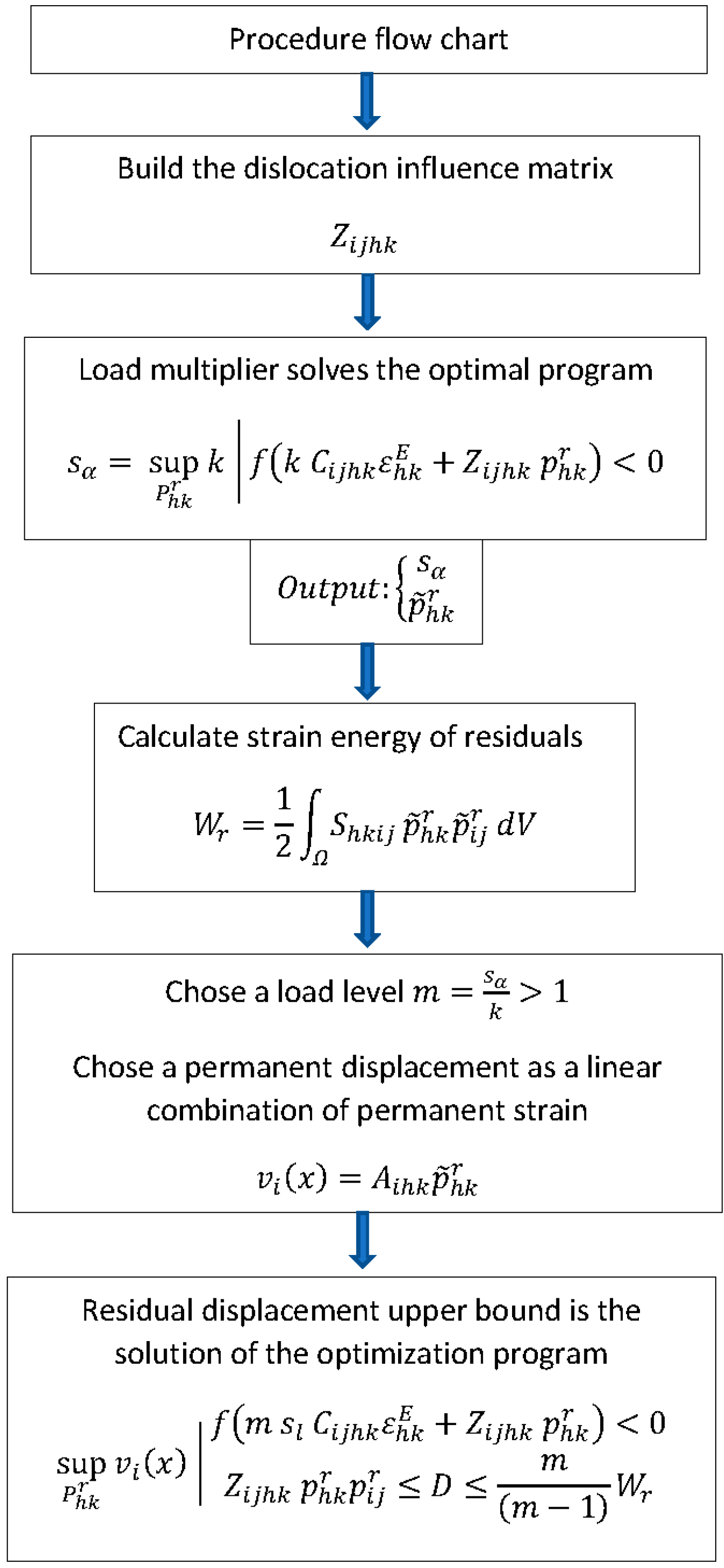
Figure 3. In
Figure 4, a flow-chart explains the numerical procedure used in the paper.
The structural scheme of the specimen is depicted in
Figure 4, where the half span length was
l = 400 mm. The mechanical constitutive constants of the specimen were reported in
Table 1, where it is illustrated only the average of the parameters.
The experimental report has furnished the relevant parameters of the material constituting the beam, and the limit bending moment has been calculated from small specimens and one span bending tests previously developed. It has to be considered that some buckling of the cross-section of the beam occurs, but the effects have been neglected in the present work [
22,
23].
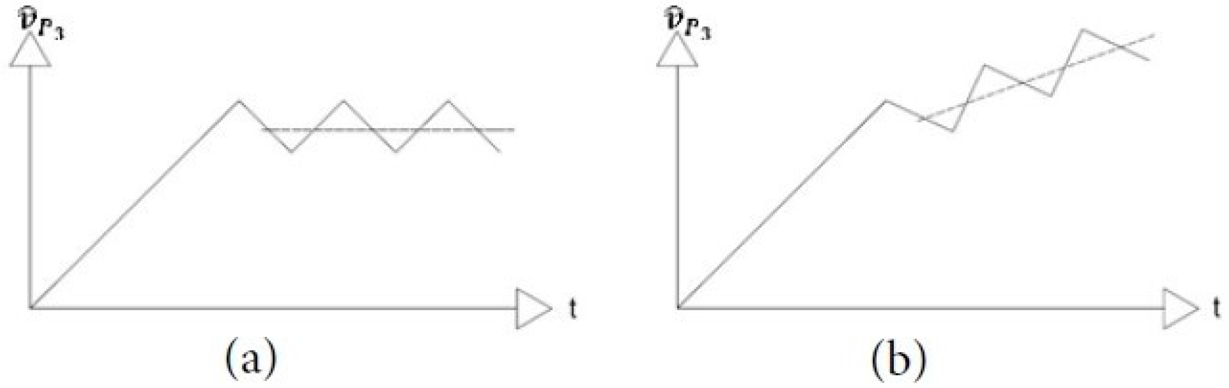
The upper bound of the load programs, , has been progressively increased from the theoretical predicted elastic limit to ratcheting. During the test, the displacement was recorded at any load step. It was possible, consequently, to record the loads for the displacement stabilized after a few cycles and ascribe it to be less than the shakedown limit. When the displacement average was increased in time indefinitely, the load bound was comprised between the shakedown and the collapse limits; however, the test was concluded when no meaningful reduction of displacement increase occurred up to 10 cycles. Finally, when the load equated to the collapse limit, the structure failed suddenly at first load application.
The cross-section of the beam was box-shaped, as reported in [
15] and in
Table 1 too, where the meaningful parameters have been highlighted.
4.1. Numerical Results
The aluminum beam described in the previous section was analyzed numerically with the proposed method.
For the calculation of the structure, the formulation reported in the previous sections must be particularized to generalized stress and strain in bending beams.
The generalized strain should be intended as the curvature of the beam’s axis and the stress the bending moment, . The bending moment is decomposed into the pure elastic moment, and the equivalent to , , residual bending moment. Finally, the permanent discontinuous strain, , is the localized rotation discontinuity, .
The first step to perform is the calculation of the Z matrix. It is pursued calculating the bending moment on the structure due to applied concentrated rotation at any point of it.
To get numerical results, at first, one must choose a discrete set of points where apply the rotation and where read the moments. To get the discrete set of points, some reasoning must be done about the variability of the response of the structure, namely:
In the proposed example, the moment varies linearly along with the structure, having discontinuous slope at the points where active or reactive forces act. Consequently, at these points, the moment is expected to have its local minimum or maximum. Those points, moreover, are a candidate to develop concentrated rotation and must be chosen as control points where one should enforce the constraints and where the dislocations must be applied. The control points are indicated with A, B, C, and D (
Figure 4). The structure is divided into four elements at points A, B, C, D, as depicted in
Figure 5. For the computational reason the calculation of all the relevant quantities involved in the routine, have been calculated at any endpoint of the elements
, as well, concentrated rotations,
, have been applied on. Moreover, the constraints of optimization Program (14) have been collocated on
, too.
The maximum elastic moment discrete values for any point have been collected in a vector and the minimum in the vector ; in the case of one monotonically increasing load pattern, .
In the same manner, the rotations
have been collected into a vector
, so that the Equation (14) transforms in a matrix form.
In Equation (21), is the negative limit bending moment vector ordered as point , and is the positive one.
The choice of the control points is dependent on the prediction of the local extrema of the internal stress. It is essential to consider that if the stress violates the compatibility equation at points not comprised in the control set, then the results overestimate the load multiplier. Consequently, one must consider setting up the procedure that converges from below in the domain of self-equilibrated stress but converges from above with the increase of the control points. In the proposed example, the position of the control points ensured that the compatibility was fulfilled everywhere in the structure.
The mechanical parameters and the geometry of the beam have been introduced into the calculation of the operator Z. Since the formulation in terms of generalized vectors of rotations and bending moments, the operator assumes the form of a square matrix here called the influence matrix. The influence matrix can be calculated directly in the case of one-dimensional structures applying the definition given in Equation (11).
The particularization of Equation (11) to the case of beams in bending gives the following representation of the residual bending moment in terms of
Z:
where the element
Zij of
Z is of the bending moment at
due to the rotation
at
.
The optimization program (21) has been solved with the data of the reported example. As a result, together with the load multiplier
, a set of rotation
is furnished, this represents the Melan residual:
Through the known Melan residual, the upper bound of the dissipation in Equation (15) is calculated as
To calculate an upper bound of the residual displacements on the structure at shakedown, the program Equation (19) has been rewritten accordingly to Positions (20) and (21).
The dissipation, in the actual case of bending, can be calculated as the sum of the partial dissipation due to the positive and negative parts of the rotations
, namely
. The objective function of the second optimization program can be assumed to be one of the desired permanent displacement in the form of a linear combination of dislocations through a constant parameters vector
.
From this position, a lower bound of the dissipated energy,
, assumes the form
For the proposed example, the resulting
Z, obtained using the assigned data, was calculated and is
| Z = | 0 | 0 | 0 | 0 | 0 | 0 | 0 | 0 |
| 0 | −4.18 × 10⁵ | −4.18 × 10⁵ | −8.36 × 10⁵ | −8.36 × 10⁵ | −4.18 × 10⁵ | −4.18 × 10⁵ | 0 |
| 0 | −4.18 × 10⁵ | −4.18 × 10⁵ | −8.36 × 10⁵ | −8.36 × 10⁵ | −4.18 × 10⁵ | −4.18 × 10⁵ | 0 |
| 0 | −8.36 × 10⁵ | −8.36 × 10⁵ | −1.67 × 10⁶ | −1.67 × 10⁶ | −8.36 × 10⁵ | −8.36 × 10⁵ | 0 |
| 0 | −8.36 × 10⁵ | −8.36 × 10⁵ | −1.67 × 10⁶ | −1.67 × 10⁶ | −8.36 × 10⁵ | −8.36 × 10⁵ | 0 |
| 0 | −4.18 × 10⁵ | −4.18 × 10⁵ | −8.36 × 10⁵ | −8.36 × 10⁵ | −4.18 × 10⁵ | −4.18 × 10⁵ | 0 |
| 0 | −4.18 × 10⁵ | −4.18 × 10⁵ | −8.36 × 10⁵ | −8.36 × 10⁵ | −4.18 × 10⁵ | −4.18 × 10⁵ | 0 |
| 0 | 0 | 0 | 0 | 0 | 0 | 0 | 0 |
The structure has been calculated for three load conditions, as reported in
Table 2.
The bending moments calculated from the load conditions are reported in
Table 3.
The collapse load multipliers for each load condition (
Table 4) are calculated by the optimization program and the shakedown multiplier as well.
Finally, the resulting Melan’s rotations are shown in
Table 5.
The second optimization program, Equation (27) is implemented to calculate the upper bound of the vertical displacement,
of point P
3. The correlation between permanent rotation and displacement is obtained by solving the structure under applied dislocation in P
3:
The result of optimization depending on
m has been reported in the following
Table 6:
As a first comparison, step by step calculation following the actual load program has given the results in terms of actual residual displacement at P
3, rotation, and dissipated energy reported in
Table 7:
4.2. Experimental Results
The experimental analysis [
15] shows the displacement record during the load path. The results have been reported here for the sake of clarity: in
Table 8, the maximum applied load, and the corresponding residual displacement of the point P
3 have been reported. The measures have been recorded when, after some cycles of loading, the displacement did cease increasing, and the load was removed,
. The measure has been repeated when the displacement,
, reduced, completing its a recovery. Finally, under the loads indicated by the (*), the displacement did not stabilize. In this case, the experiment finished after many cycles, and the residual displacement has been recorded. Even in this case, a new measure has been recorded after time to keep the memory of the recovering effect.
Table 8 contains the experimental results, as reported in [
15].
The experimental results denote that the actual residual displacements are greater than the calculated through step by step procedure. Indeed, in the analysis, the average limit bending moment has been used, the experimental report describes that the qualification tests to evaluate the mechanical properties of the specimens, produced non-uniform results and the average reported value, as shown in
Figure 6, is affected by a meaningful standard deviation.
In conclusion, during the experiment, the structure underwent to ratcheting for loads greater than 2.099 kN. The recorded displacement rate did not vanish, and the measured values refer to the end of the experiment. For loading less to 2.099, the permanent displacement increment vanishes definitely, i.e., it tends to remain constant in time after two or three cycles; hence, the shakedown has occurred. The proposed method has been applied to the structure; the program Equation (21) has been used to calculate the shakedown multiplier and the residual rotations.
Moreover, the resulting Melan’s residuals have been introduced to formulate the program Equation (27), where the displacement in the middle of the right span has been calculated in terms of the residual rotation. The upper bound of the displacement has been calculated for two different values of the factor
m.
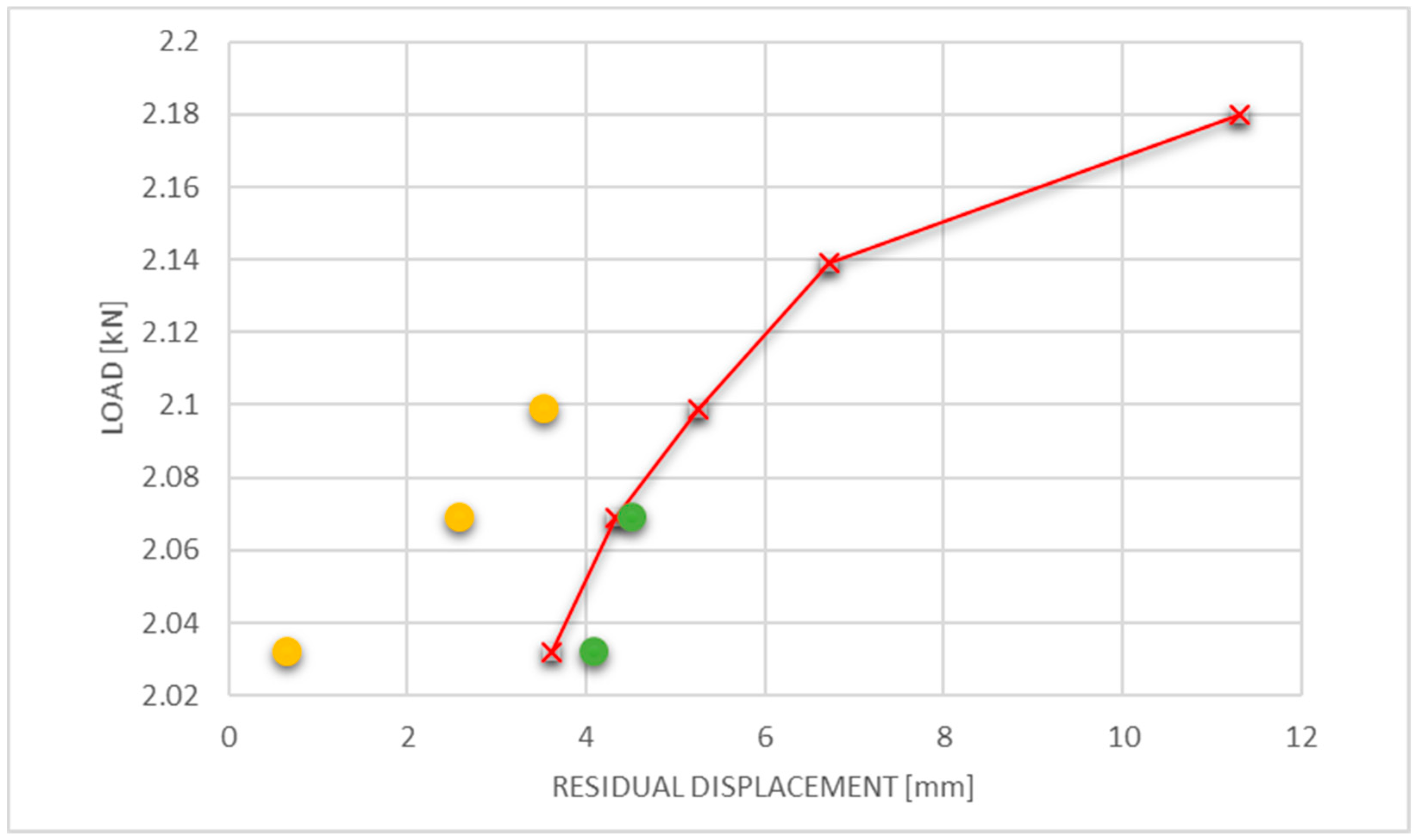
Table 9 contained the comparison between the experimentally recorded displacement and the upper bound calculated through the present proposed procedure.
Figure 7. represents the load-displacement experimental curve, where the calculated displacement upper bound has been reported.


