Integration of Wavelet Denoising and HHT Applied to the Analysis of Bridge Dynamic Characteristics

1
School of Geodesy and Geomatics, Wuhan University, Wuhan 430079, China
2
Key Laboratory of Mine Spatial Information Technologies of National Administration of Surveying, Mapping and Geo-information, Henan Polytechnic University, Jiaozuo 454000, China
3
Collaborative Innovation Center of Geospatial Technology, Wuhan 430079, China
4
Licheng Branch of Ji’nan Natural Resources and Planning Bureau, Ji’nan 250100, China
*
Author to whom correspondence should be addressed.
Appl. Sci. 2020, 10(10), 3605; https://doi.org/10.3390/app10103605
Submission received: 5 April 2020
/
Revised: 14 May 2020
/
Accepted: 18 May 2020
/
Published: 22 May 2020
(This article belongs to the Special Issue Advances on Structural Engineering)
Abstract
:When the dynamic characteristics of a bridge structure are analyzed though Hilbert–Huang transform (HHT), the noise contained in the bridge dynamic monitoring data may seriously affect the performance of the first natural frequency identification. A time-frequency analysis method that integrates wavelet threshold denoising and HHT is proposed to overcome this deficiency. The denoising effect of the experimental analysis on the simulated noisy signals proves the effectiveness of the proposed method. This method is used to perform denoising pre-processing on the dynamic monitoring data of Sutong Bridge, and the denoised results of different methods are compared and analyzed. Then, the best denoising data are selected as the input data of Hilbert spectrum analysis to identify the structural first natural frequency of the bridge. The results indicate that the wavelet-empirical mode decomposition (EMD) method effectively reduces the interference of random noise and eliminates useless intrinsic modal function (IMF) components, and the excellent properties of the signal evaluation index after denoising make the method suitable for processing non-stationary signals with noise. When Hilbert spectrum analysis is applied to the denoised data, the first natural frequency of the bridge structure can be identified clearly and is consistent with the theoretical calculation. The proposed method can effectively determine the natural vibration characteristics of the bridge structure.
1. Introduction
Affected by ambient excitation and traffic loads, the complex structure of long-span bridges may have internal and non-linear responses that influence the health of bridge structures. The analysis of the dynamic characteristics of bridge structures under various conditions through the health monitoring of large bridges is essential to the construction and safe operation of bridges. As an important parameter reflecting the dynamic characteristics of bridge structures, the main vibration frequency has become the focus of attention in bridge monitoring. Many studies have showed that the modal frequencies of different structures and their changes reflect the health state of a bridge structure [1,2,3,4,5,6,7,8]. The accelerometers, optical fibers, piezoelectric sensors, and intelligent materials attached to important components of a bridge structure can monitor their local natural frequency characteristics [1,2,3,4,5,6,7,8,9]. However, the displacement deformation characteristics are difficult to determine [9,10,11]. Although total station (even robotic total station), 3D laser scanners, close-range photogrammetry equipment, and the Global Navigation Satellite System (GNSS) have been adopted to monitor the deformation information of bridges, their respective shortcomings limit their wider application [10,11,12,13]. Nakamura [14] used GNSS technology in 1998 to monitor the dynamic deformation of a suspension bridge with a main span of 720 m and verified that the vibration displacement and main frequency of the main beam under wind load were consistent with the results of the wind tunnel experiments and finite element calculations. Given that GNSS monitoring can provide long-term, continuous, high-frequency, and dynamic displacement information and extract dynamic frequencies from it, GNSS technology has become an important means of bridge health monitoring and is widely used in the safety monitoring of bridge structures [15,16,17,18,19].
GNSS dynamic observation data often contain considerable noise due to the interference of external environmental factors, such as multipath effects, and noise-containing GNSS signals usually exhibit nonlinearity and non-stationarity. Thus, exploring the abundant structural health information hidden in GNSS monitoring signals is crucial. Domestic and foreign scholars have conducted studies on non-stationary signal processing methods, such as short-time Fourier transform, wavelet transform, and the Wigner–Ville distribution [20,21,22,23,24]. Although short-time Fourier and wavelet transform can analyze the time-frequency characteristics of non-stationary noise-containing signals, these methods on non-stationary signals may lead to the phenomenon of false components due to the limitation imposed by the uncertainty principle. In addition, the selection of the Fourier window and wavelet basis functions entails high subjectivity, which limits the utilization scope of the two methods to some extent [25]. Hilbert–Huang transform (HHT) is an adaptive local time-frequency analysis method proposed by Huang et al. in 1998; HHT is composed of empirical mode decomposition (EMD) and the Hilbert transform (HT) [26]. The method carries out blind adaptive decomposition in accordance with the signal itself and separates the non-stationary signal into several intrinsic mode functions (IMF) according to the frequency content (from high to low frequency). On this basis, HT is implemented on each IMF component to explore its spectral characteristics [26]. However, due to the influence of noise and signal discontinuity, the mode-mixing problem often occurs when EMD is applied to the decomposition of non-stationary noise-containing signals. This may result in interference on the EMD decomposition results and the subsequent results of Hilbert spectrum analysis; consequently, effective physical information may not be accurately determined [27,28]. Xu et al. [29] improved the HHT method, applied it to the processing of the GNSS monitoring data of Baishazhou Yangtze River Bridge in Wuhan, and verified the effectiveness and rationality of this method when used for modal parameters’ identification from non-stationary vibration signals.
With regard to the development of EMD-related algorithms, Wu et al. [30] proposed a noise-assisted data analysis method called ensemble empirical mode decomposition (EEMD), which suppresses the mode mixing problem of EMD by adding white noise to the initial data many times. However, the performance of the EEMD algorithm depends largely on the noise amplitude and the number of trials. The IMFs generated by EEMD become highly polluted and even yield pseudo-components when noises with inappropriate amplitudes are added and the number of trials is changed inappropriately [31]. Furthermore, the time required by EEMD-related algorithms may increase when the number of trails is increased [32].
On the basis of the remarkable effect of noise when the HHT method is applied to non-stationary data and in consideration of the excellent time-frequency localization properties in the field of filtering and denoising, a time-frequency analysis method based on the combination of wavelet threshold denoising and HHT is proposed in this study. The GNSS dynamic monitoring data of Sutong Bridge are adopted as the study object, to identify the first natural frequency of the bridge structure. The implementation process is presented.
The method implements noise reduction preprocessing on the dynamic monitoring data to obtain reduced decomposition layers in the EMD decomposition process and decrease the marginal effects on the quality of useful signal decomposition. The vibration component is reconstructed according to the correlation of each component and subsequently serves as input data for Hilbert spectral analysis to identify the first natural frequency of the bridge structure. The denoising effect of the experimental analysis on simulated noisy signals proves the effectiveness of the proposed method. The application analysis results of real bridge monitoring data indicate that the proposed method can highlight the dynamic characteristics of bridge structure vibration signals in noisy environments and effectively identify the first natural frequency, which is conducive to the scientific evaluation of the safety status of the bridge structure.
2. Basic Principle of HHT
Hilbert spectrum analysis is performed using HHT from the non-stationary signal. The HHT-based time-frequency analysis method consists of two main steps: (1) multi-scale decomposition, which is implemented on non-stationary signals using the EMD method and whose result is a series of IMFs, and (2) HT, which is performed on each IMF component represented in the joint time-frequency domain. Then, the Hilbert spectrum of the signal is acquired. The steps of EMD method [26,27,28] are as follows:
(1) The extreme points of non-stationary signal x(t) are fitted using the cubic spline function mentioned in [26] to obtain the upper and lower envelopes of the signal. The mean is calculated as:
(2) The remainder is calculated as:
Afterwards, whether satisfies the definition of IMF is determined [26]. If the definition is satisfied, then is the first IMF component and denoted as:
where is the value of after the kth iteration. Otherwise, iterative calculation continues until the condition mentioned in [26] is met.
(3) is separated from . Then, a differential signal with the high-frequency components removed is obtained as follows:
(4) The preceding steps are repeated many times by taking (the latter counterpart is recorded as ) as a new signal [26], and the individual IMF components are decomposed sequentially. The decomposition process terminates when residual signal is a monotonic function. Then, is decomposed into n IMF components and one remainder through the above-mentioned method.
The decomposition process shown above indicates that the EMD model separates the non-stationary signal into several intrinsic mode functions, which are all stationary or stationary-trended signals (i.e., it is an adaptive signal decomposition method). The obtained indicates that the original signal is decomposed into components with different frequency scales. is the tendency part, and the decomposition result is related only to the original signal.
HT is carried out on each IMF decomposed from Equation (2) as follows:
The analytic signal is constructed as:
The amplitude function is obtained as:
Furthermore, the instantaneous frequency is described as:
Therefore,
where Re is the real part of the original signal, and residual function can be ignored.
Equation (10) is the Hilbert spectrum, which is recorded as:
The Hilbert marginal spectrum is defined as:
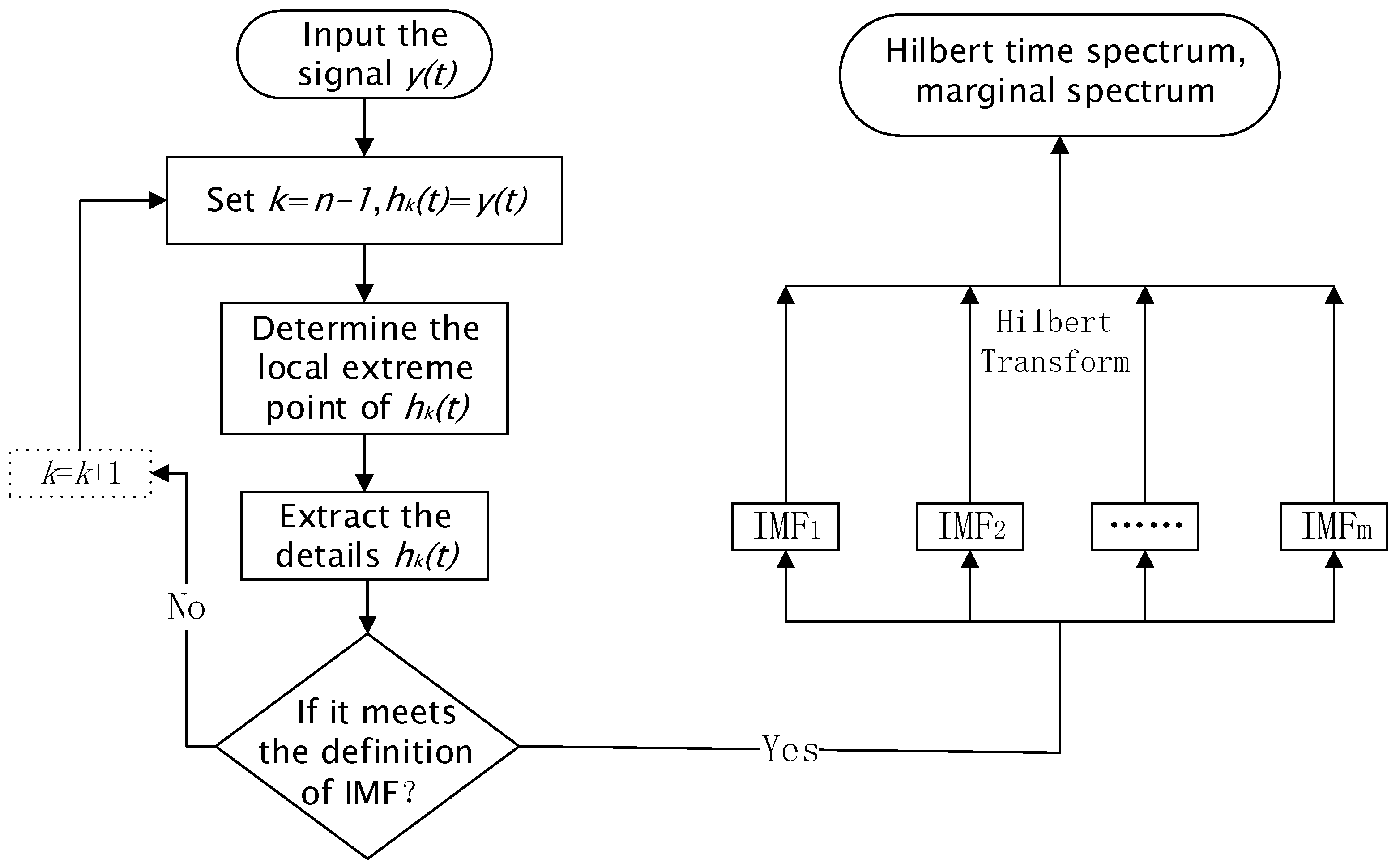
where T represents the total length of the signal, indicates that the signal amplitude varies with the change in time and frequency within the entire frequency range, and shows that the signal amplitude varies with the change in frequency. When the energy of a certain frequency appears in or , the vibration wave of this frequency appears. Thus, the Hilbert marginal spectrum can accurately reflect the actual frequency component of the signal. The flow of non-stationary data processing using the HHT method is shown in Figure 1.
3. Time-Frequency Analysis Method Based on Wavelet Threshold Denoising and HHT
In real engineering applications, the dynamic observation data collected from the GNSS receiver may contain many components aside from the vibration signals from the bridge structure itself, and the data may also contain interference from environmental noise. Therefore, the signal-to-noise ratio (SNR) is relatively low, which greatly affects the recognition accuracy of the main vibration frequency. Only by filtering out noise effectively can useful information and reasonable and reliable conclusions be obtained. For the EMD method, the modal aliasing phenomenon may occur due to intermittent events and the interaction between signals, resulting in incomplete decomposition. The number of decomposition layers from the EMD decomposition process and the margin effect on signal analysis must be reduced via denoising pre-processing to improve the accuracy and timeliness of signal feature extraction.
3.1. Wavelet Threshold Denoising
The wavelet threshold method is popular in signal denoising, whose basic idea is to denoise the non-stationary signal as follows: Firstly, multi-scale decomposition is performed on the noise-containing signal. Secondly, an appropriate threshold function is selected to threshold the wavelet coefficients. Lastly, the inverse wavelet transform is used to reconstruct each signal and achieve denoising. If signal f(t) is a square integrable function, then the wavelet transform of f(t) is the inner product of the signal and wavelet function :
where a represents the scale factor, b represents the translation or displacement factor, , and the conjugate function of is denoted as . Wavelet transform analyzes signal by scaling and shifting the position of . Thus, the wavelet transform results possess good time- and frequency-domain localities when the wavelet function is selected properly. Selecting the appropriate threshold function in the practical application of wavelet threshold denoising is extremely important because it minimizes the noise in noisy data and preserves the local characteristics of the effective signal. Although hard and soft threshold denoising methods are widely used in data filtering, they still have shortcomings. The works in [25,26,27,28,29] proved that the semi-threshold function shown in Equation (14) may obtain good denoising results.
where is the Bayesshrink thresholding, , and C is a constant that usually has a value greater than one. The threshold function has continuity and high-order conductivity. It overcomes the discontinuity and oscillation problems of the signal reconstructed from the hard threshold function and addresses the deficiency that although the soft threshold function is continuous, the denoising results need to be subtracted from the threshold; systematic deviation exists when the coefficient exceeds the threshold.
3.2. Time-Frequency Analysis Method Combining Wavelet Threshold Denoising and HHT
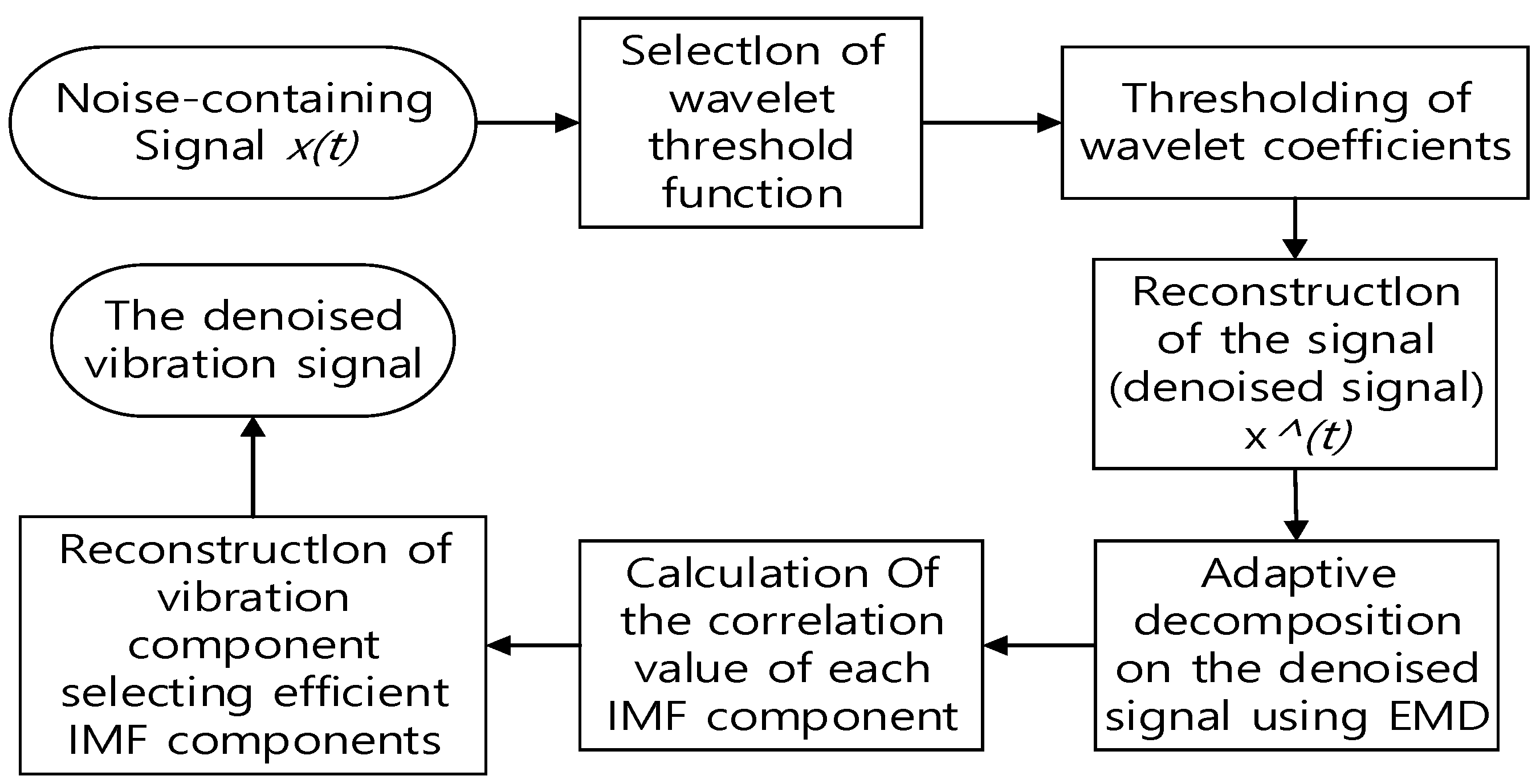
Although the wavelet threshold method can eliminate white noise in the original signal, the noise reduction preprocessing may not sufficiently eliminate the interference of noise in practical applications due to the noise interference of many different properties. Therefore, the IMF correlation must be adopted for appropriate post-processing, and it may improve the recognition accuracy of the main vibration frequency. The denoising method based on wavelet threshold denoising and EMD is called the wavelet-EMD method, and its specific steps are as follows:
(1) Wavelet threshold denoising: To eliminate the influence of noise, the original noise-containing non-stationary signal is decomposed by the wavelet threshold, and the signal is reconstructed according to the energy of the decomposed frequency band. The denoising signal that eliminates interference noise is then obtained. This denoising process via the wavelet threshold can decrease the influence of high-frequency noise and the decomposition layers of EMD. Hence, it may provide a relatively “clean” input signal for EMD.
(2) Multi-scale EMD is carried out on the denoised signal processed by the wavelet threshold denoising method to obtain the IMF components of the denoised signal, .
(3) The correlation value of each IMF component is calculated to identify the vibration component of the bridge structure.
For the decomposition results of large-scale building dynamic observation data, the high-frequency parts of the IMF component are generally dominated by noise, and the low-frequency part is dominated by the vibration signal. The investigation of the decomposition results of EMD indicates that several components have little energy after decomposition and cannot represent the original signal, which is not conducive to analyzing the spectral characteristics of the signal. To identify the effective vibration component easily, the component correlation according to the correlation between each component and the original signal is defined to distinguish the effective IMF component from the unwanted IMF component.
where represents the ith IMF component of the signal and represents the corresponding residual signal. The residual signal corresponding to the ith component is obtained as:
where represents the original signal. The definition implies that the correlation of the IMF components reflects the correlation of each component with the original signal and can be used to identify components with different physical meanings.
(4) Reconstruction of the vibration component. The decomposed components are selected based on the correlation value and actuquaal demand. The useless IMF component is eliminated, and the effective IMF component is used for reconstruction to obtain the denoised vibration signal.
The flow of time-frequency analysis via the wavelet-EMD method is shown in Figure 2.
The quality of denoising performance is the key to evaluating the advantages and disadvantages of a denoising algorithm in practical applications. Therefore, an objective denoising performance evaluation index must be selected. Similar to the evaluation index of image denoising [33], the root mean squared error (RMSE) and SNR are usually chosen for such an evaluation. RMSE and SNR are expressed as follows:
where is the denoised signal, is the original signal that serves as the standard signal, and N is the length of the signal. RMSE reflects the proximity of the denoised signal to the original signal. The smaller the value is, the more obvious the obtained filtering effect is. Meanwhile, SNR reflects the ratio between the denoised and the noisy signal, and its value symbolism is contrary to that of RMSE. With regard to the denoising the bridge GNSS dynamic observation data, the pre-processing of dynamic data must retain the useful signal as much as possible whilst removing the noise to the greatest extent. Thus, the two evaluation indicators must be considered together when evaluating the denoising effect of non-stationary signals. That is, the RSME of the denoised and original signals and the SNR of the filtered signal should meet the requirements.
3.3. Comparative Analysis of the Denoising Effect on Simulation Signals
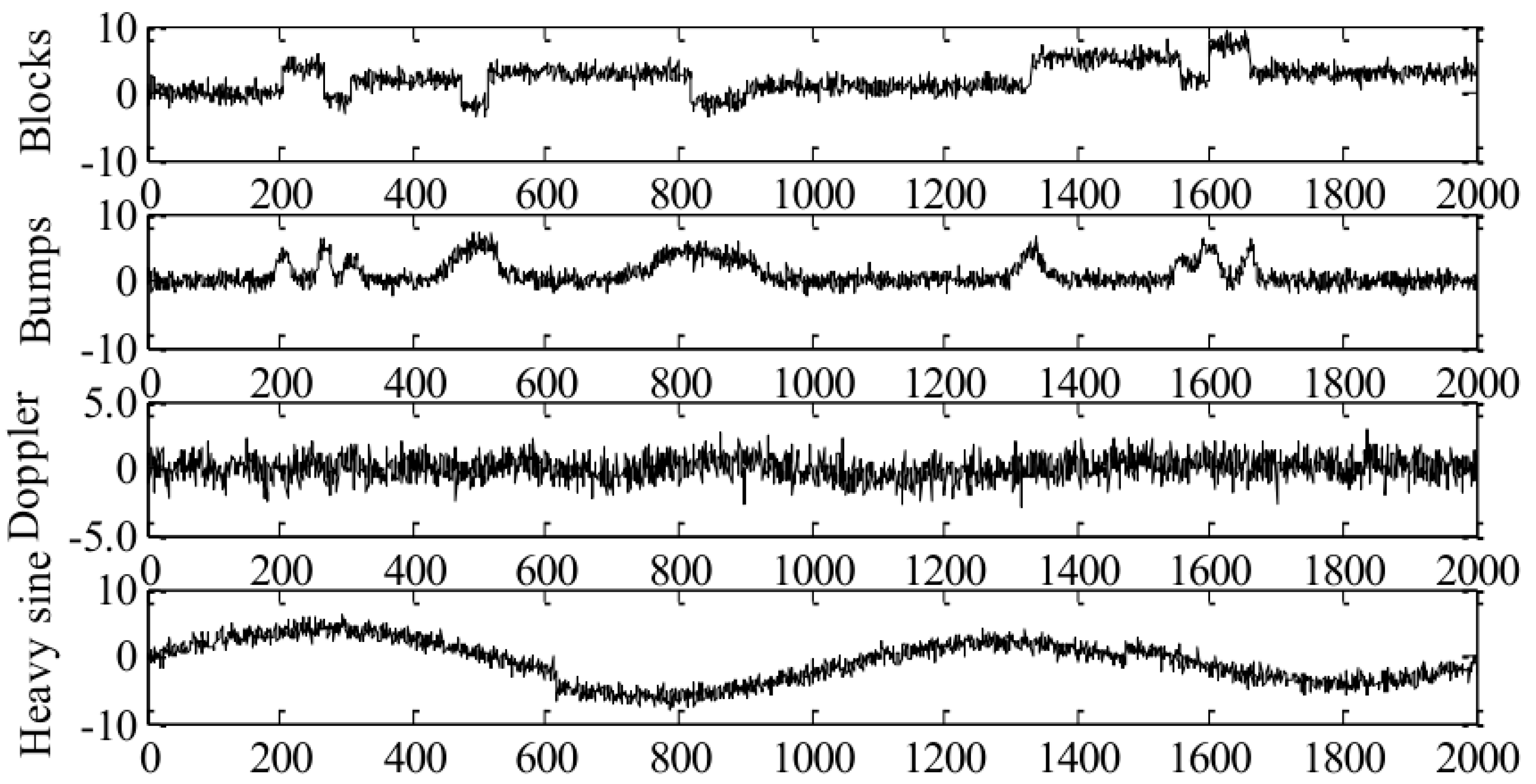
Several commonly used standard analogue signals, such as the blocks, bumps, Doppler, and heavy sine signal, were selected for a simulation analysis, which aimed to verify the performance of the proposed denoising method and examine the effective suppression of the modal aliasing phenomenon in the traditional EMD method. The denoising performance of the proposed method was compared with that of wavelet denoising and EMD methods. The two evaluation indicators were used to evaluate the denoising performance of the four methods quantitatively.
Classic simulation signals were generated by the Wnoise function in MATLAB 2014b. These signals had the same sampling length and different SNR. Their waveforms (SNR were all 4 dB) are shown in Figure 3.
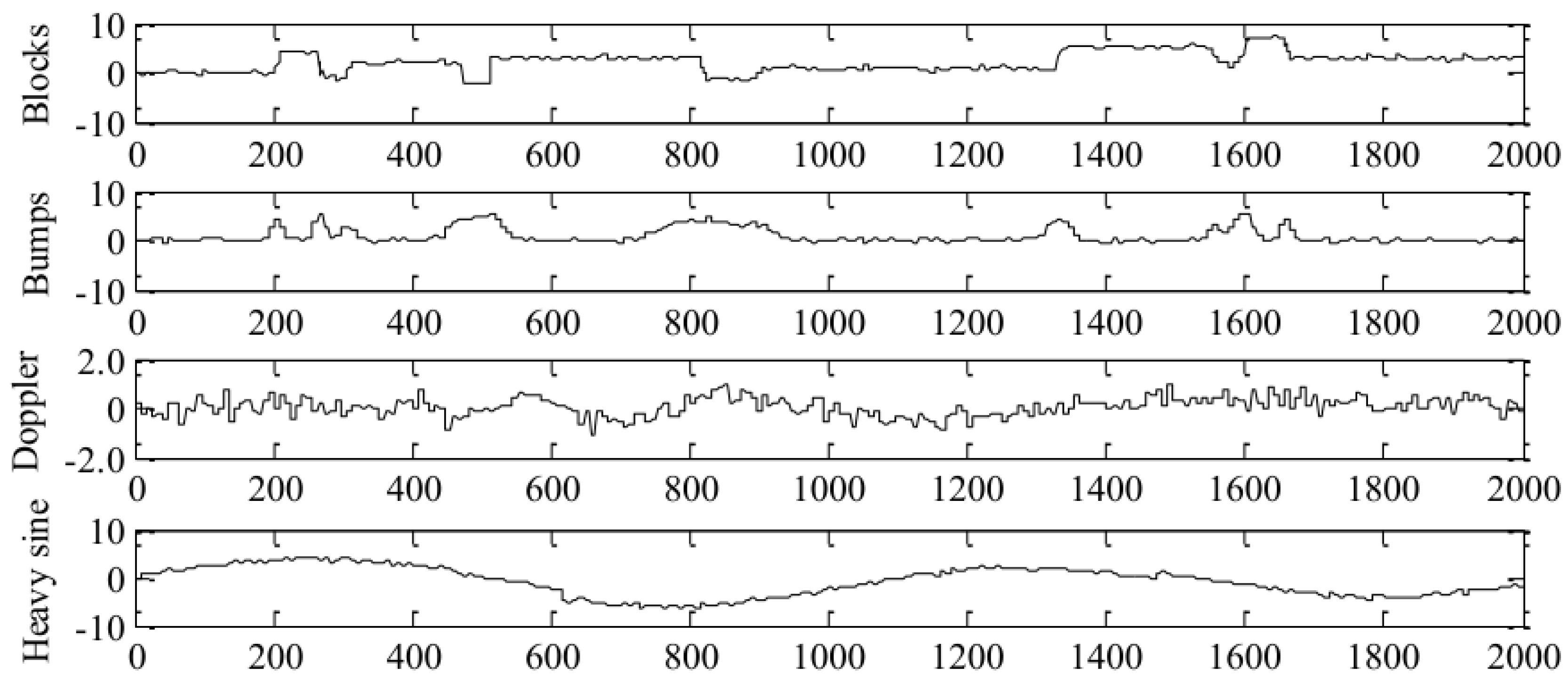
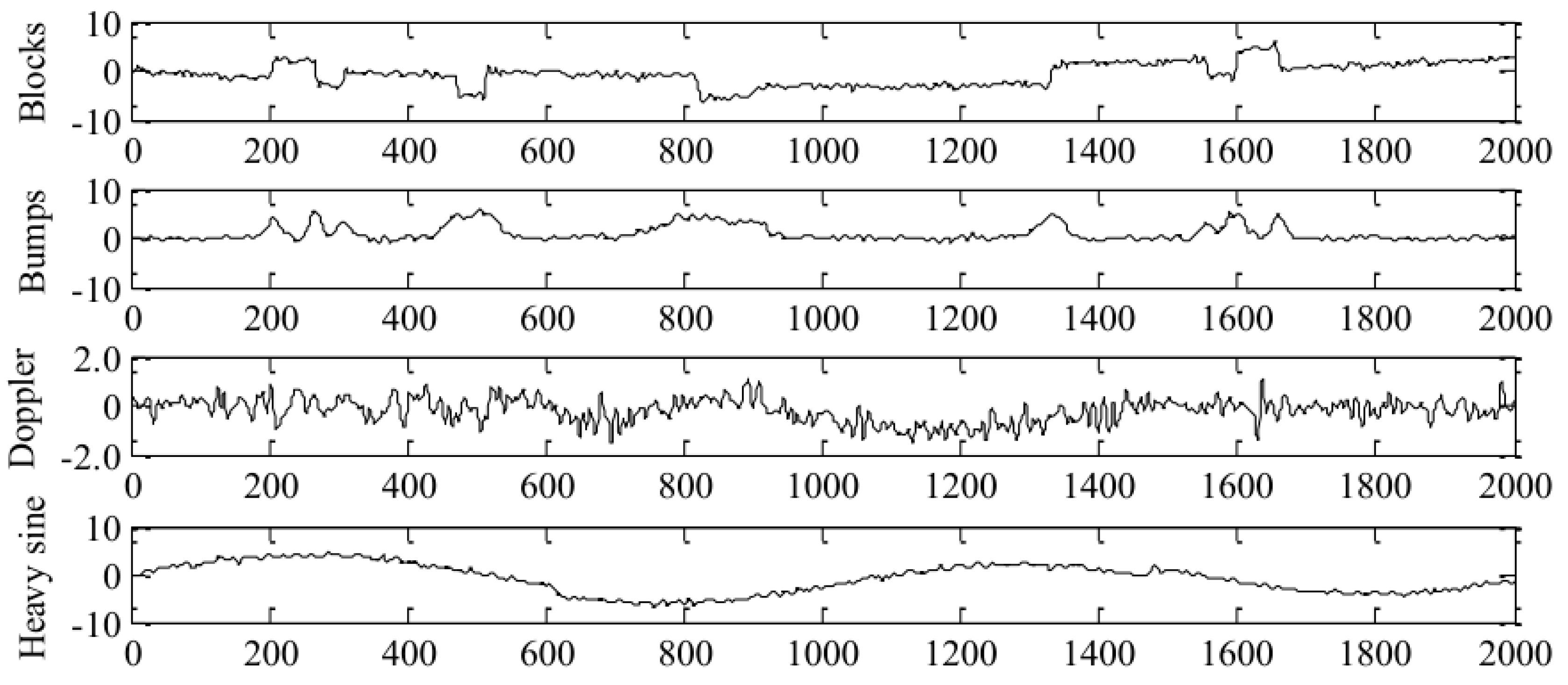
Figure 4, Figure 5 and Figure 6 indicate that all of the methods had certain filtering and denoising effects. However, identifying which method performed better than the others was difficult. The RMSE and SNR of the three methods are calculated and listed in Table 1.
Table 1 indicates that each method performed well to a certain degree in terms of the denoising effect on the simulation signals. Overall, the denoising effect of the wavelet denoising method was not as good as that of EMD and was inferior to that of wavelet-EMD. The wavelet-EMD method performed well not only in the evaluation indicator SNR, but also in RMSE, thereby satisfying the demands mentioned in Section 3.2.
To investigate this issue further, noisy signals with different SNRs (i.e., 6, 2 and −2dB) were analyzed in the same manner as above. The wavelet functions for the comparative analysis used the db8 function and the semi-soft threshold method. The waveforms of the denoising results from the different methods were omitted to save space; only the denoising effect indicators after processing are listed in Table 2.
Table 2 together with Table 1 show that the denoising effect of the different methods was verified again. Several conditions were inapplicable to the blocks signal. The denoising effect varied with the SNR of the noisy signal. The wavelet-EMD method exhibited good adaptability, and its denoising effect had little correlation with the noise intensity of the noisy signal. In particular, even when the SNR of the noisy signal was relatively low, the denoising result from the wavelet-EMD method was smooth, and the method could still denoise effectively. The superiority of the proposed algorithm was proven again.
4. Application Analysis
Sutong Bridge, which is in the lower reaches of Yangtze River, is a steel box girder cable-stayed bridge with double towers and double cables. Its main span is 1088 m long, and its main tower is 300.4 m high. Sutong Bridge ranked second amongst similar-type bridges in the world at the time of its completion. Evaluating the stage line shape, force, and safety of the bridge structure and determining the safety status of the bridge structure under environmental excitation conditions are vital. An all-weather dynamic geometric monitoring system based on GNSS technology had been established to monitor the geometry and structural state of towers and beams continuously and in real-time, to analyze the construction status, and to avoid unfavorable construction conditions [16]. The GNSS monitoring points were set synchronously according to the needs of construction control and monitoring during the installation process of the steel box girder. The overall layout of the monitoring points is shown in Figure 7.
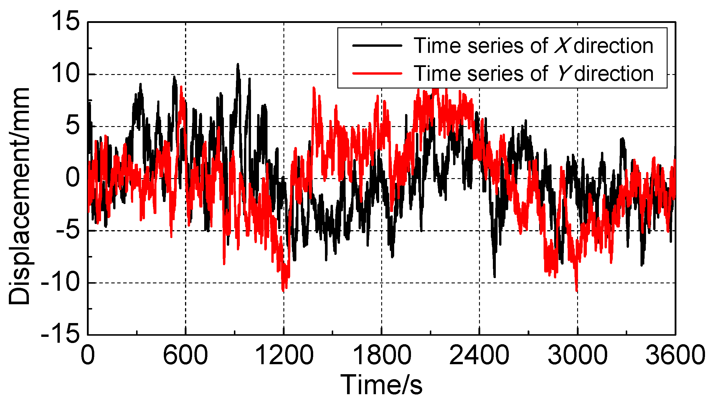
The experimental data were obtained from the monitoring of a point on Sutong Bridge under a normal construction environment on 1 May 2007; the weather condition was good; the altitude cut-off angle of the satellites was set to 15°; and the continuous observation in the dynamic observation mode lasted for approximately 3 h. Given that the natural frequency of long-span bridges usually falls within the range of 0–2 Hz, the monitoring sequence with the frequency range of 0–5 Hz could be identified when the sampling frequency of the GPS receiver was set to 10 Hz according to the Nyquist sampling theorem of signal processing. This identified range satisfied the requirements of first natural frequency identification. The GNSS dynamic observation data included the vibration signal of the bridge structure under environmental excitation and accidental errors, such as the multipath effect, because of the influence of the construction and the natural environment. Therefore, the rich bridge structure health information embedded in GNSS monitoring signals must be mined. The observation sequences of the monitoring point in the x (lateral) and y (longitudinal) directions lasting for 1 h were selected to identify the first natural frequency of the bridge structure using the proposed method and to analyze the dynamic characteristics of the bridge structure. The obtained coordinate sequence was transformed from a geodetic coordinate system into a bridge axis coordinate system by using the same method as that in [11]. The time history curve of the averaged data from the GNSS monitoring point is shown in Figure 8. The accuracy analysis of the observation sequence in [16] indicated that the horizontal and vertical mean square errors in the entire time period were mm and mm. These values implied that no large gross errors existed amongst the observation values, and the accuracy of the GNSS dynamic observation data was reliable and suitable for dynamic frequency extraction.
4.1. Comparative Analysis of the Denoised Results
Figure 8 shows the observation sequence of a monitoring point on the bridge in horizontal and vertical directions, but the vibration characteristics of the bridge structure cannot be determined visually. Under the interference of factors such as noise, the accuracy and effect of the identification of the first natural frequency of the bridge structure may be influenced if the original observation data were directly used for the dynamic characteristic analysis. Therefore, performing denoising pre-processing on the original observation sequence was necessary to improve the accuracy of identifying the first natural frequency. In the experiment, the wavelet-EMD denoising method based on wavelet threshold denoising and the EMD method were used to denoise the observation sequence in the horizontal and vertical directions in Figure 8. The results were compared with those of hard, soft, and semi-threshold wavelet denoising (the wavelet function selects the Sym wavelet, and the decomposition layer selected four layers; the wavelet-EMD method used the semi-threshold function). The results of the four denoising methods are shown in Figure 9, where H-Wavelet represents hard threshold denoising, S-Wavelet represents soft threshold denoising, I-Wavelet represents half threshold denoising, and WE represents wavelet-EMD denoising. Figure 9a shows the denoising results in the horizontal direction obtained using the four methods, and Figure 9b shows the denoising results in the vertical direction derived with the four methods.
Figure 9 shows that the wavelet-EMD method obtained a large reduction in Gaussian white noise in the horizontal and vertical directions compared with the three other methods. The signal denoised by the wavelet-EMD method also filtered out most of the invalid IMF components, which could highlight the original signal information. The SNR and RMSE of the denoised signal and the linear correlation coefficient between the denoised signal and the original observation sequence were calculated to evaluate the denoising performance of the four methods quantitatively. Table 3 shows a comparison of the denoising performance of the four methods in the horizontal and vertical directions.
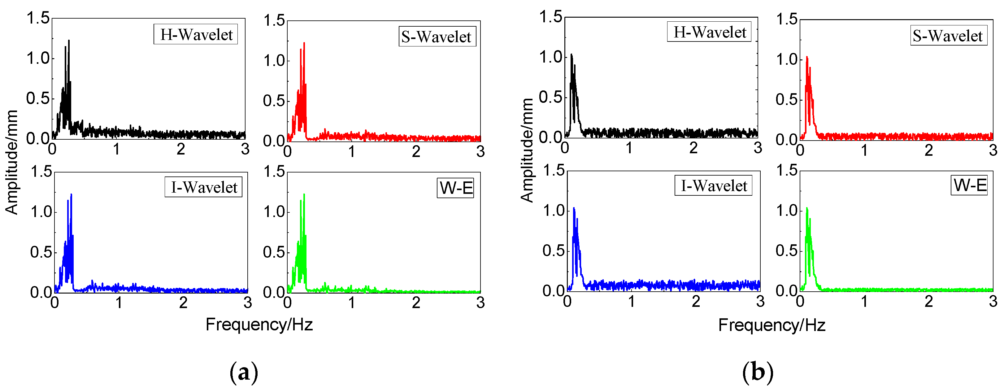
A comparative analysis of Figure 9 and Table 3 indicates that all four denoising methods played a certain denoising role, but the denoising effects differed slightly in different directions. In the comparison of the H-Wavelet and S-Wavelet methods, the three evaluation indexes indicated that the H-Wavelet method had a better denoising effect in the horizontal direction, whereas the S-Wavelet denoising method had a better denoising effect in the vertical direction. The wavelet-EMD method exerted a stable denoising effect in both directions. The method had a lower RMSE of the denoised signal and a higher SNR than the three methods, thus suppressing the noise effectively. This result proved that wavelet-EMD achieved the best denoising effect amongst the four methods. In addition, the linear correlation coefficient between the denoised and original observed signals in Table 3 indicated that the correlation between the signal denoised by the H-Wavelet method and the original signal was the weakest; the correlation between the denoised signal using the wavelet-EMD method and the original signal was the strongest, which also reflected the good denoising performance of the wavelet-EMD method. The spectral values of the signals in the horizontal and vertical observation sequences denoised by the four methods were calculated to compare the methods’ denoising performance further. The results are shown in Figure 10.
The comparative analysis of the spectral values of the denoised signals from the four methods in Figure 10a,b indicated that the main frequencies of the observed sequences filtered by the four methods were prominent, which meant that these methods played a certain role in noise inhibition. However, the noise spectrum power of the denoised signal via the H-Wavelet and S-Wavelet methods was relatively large, and the frequency of the noise still filled the entire frequency band. The noise spectrum power of the denoised signal via the I-Wavelet method was reduced to a certain extent, and the noise spectrum power was the smallest in the case of the wavelet-EMD method. Noise was suppressed well in the high-frequency band greater than 2 Hz, indicating that the method effectively removed the interference of noise. Thus, the denoised data obtained by the wavelet-EMD method served as the input data of the Hilbert spectrum analysis in this study to extract the first natural frequency of the bridge structure.
4.2. First Natural Frequency Identification from the Denoised Results
Given that the HT method was sensitive to errors during spectral analysis, the accuracy of Hilbert spectrum analysis could be improved to some extent if the quality of the original observation data were improved by appropriate data preprocessing methods. Therefore, the “clean” monitoring sequence after denoising that served as the input data was vital for the identification of the main vibration frequency of the bridge structure, which was why noise reduction pre-processing of the dynamic observation data was performed in Section 4.1. In this section, the Hilbert spectrum analysis is performed on the observed data sequence after denoising, and the vibration frequencies of the bridge structure in the horizontal and vertical directions are identified. Meanwhile, the identification value in this study and the empirical calculation value must be compared to determine the health and structural safety status of the bridge, which would verify the reliability and accuracy of the first natural frequency identification result.
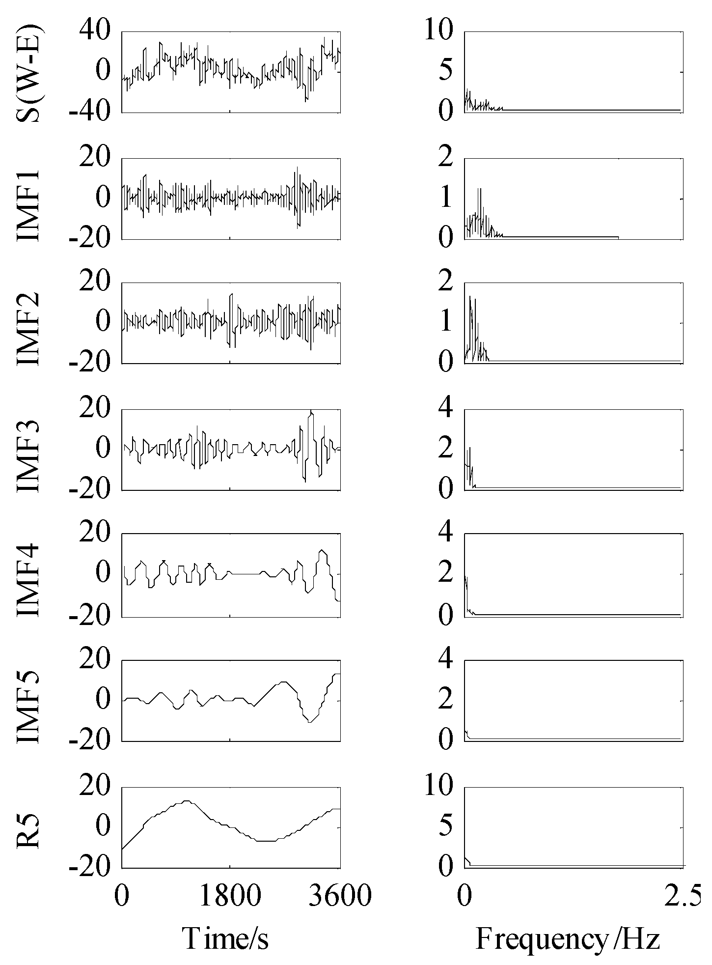
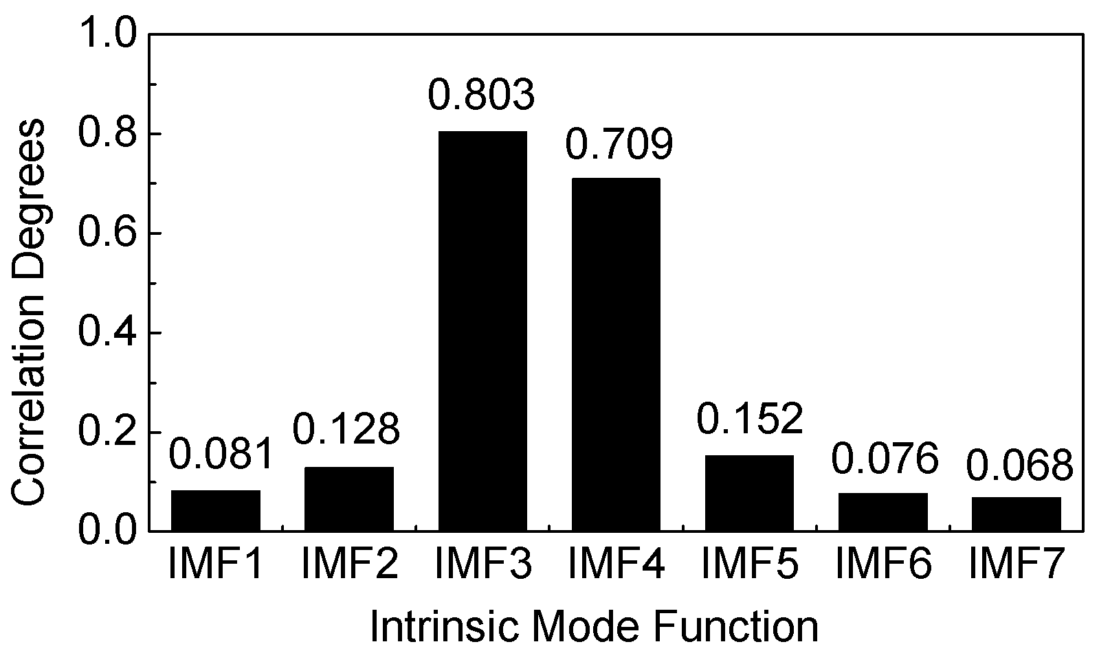
The EMD process was implemented on the original noise-containing observation sequence in the horizontal direction of the bridge, then on the denoised signal via the wavelet-EMD method. The purpose was to verify that the time-frequency analysis method based on wavelet threshold denoising and HHT could effectively extract the first natural frequency of the bridge structure under a noisy environment and that the dynamic characteristic analysis was feasible. Each IMF and the remainder in the time- and frequency-domains are shown in Figure 11 and Figure 12 (S represents a noisy observation sequence in the horizontal direction and S(W-E) represents the denoised signal using the Wavelet-EMD method), and the correlation values of the respective IMF components were calculated simultaneously and shown in Figure 13 and Figure 14.
A comparative analysis of Figure 11 and Figure 13 indicates that the frequencies of IMF1 and IMF2 components obtained from the EMD method before denoising were distributed in a disorderly manner, and the correlation value of the component was low. IMF1 and IMF2 were high-frequency noise components according to the global and high distribution of the accidental error. Figure 12 shows that the high-frequency noise in the original observation sequence was suppressed effectively via wavelet-EMD denoising, and the number of decomposition layers of EMD was decreased. Given that the natural frequency of a long-span bridge structure is low, which is generally in the range of 0.1–1 Hz [29], the correlation values of the first three IMF components of the denoised signal were high, and those of the last two IMF components were low (Figure 14). Therefore, invalid trend components IMF4 and IMF5 may be removed from the denoised signal, and effective components IMF1–IMF3 were selected for reconstruction to obtain the vibration component of the bridge structure.
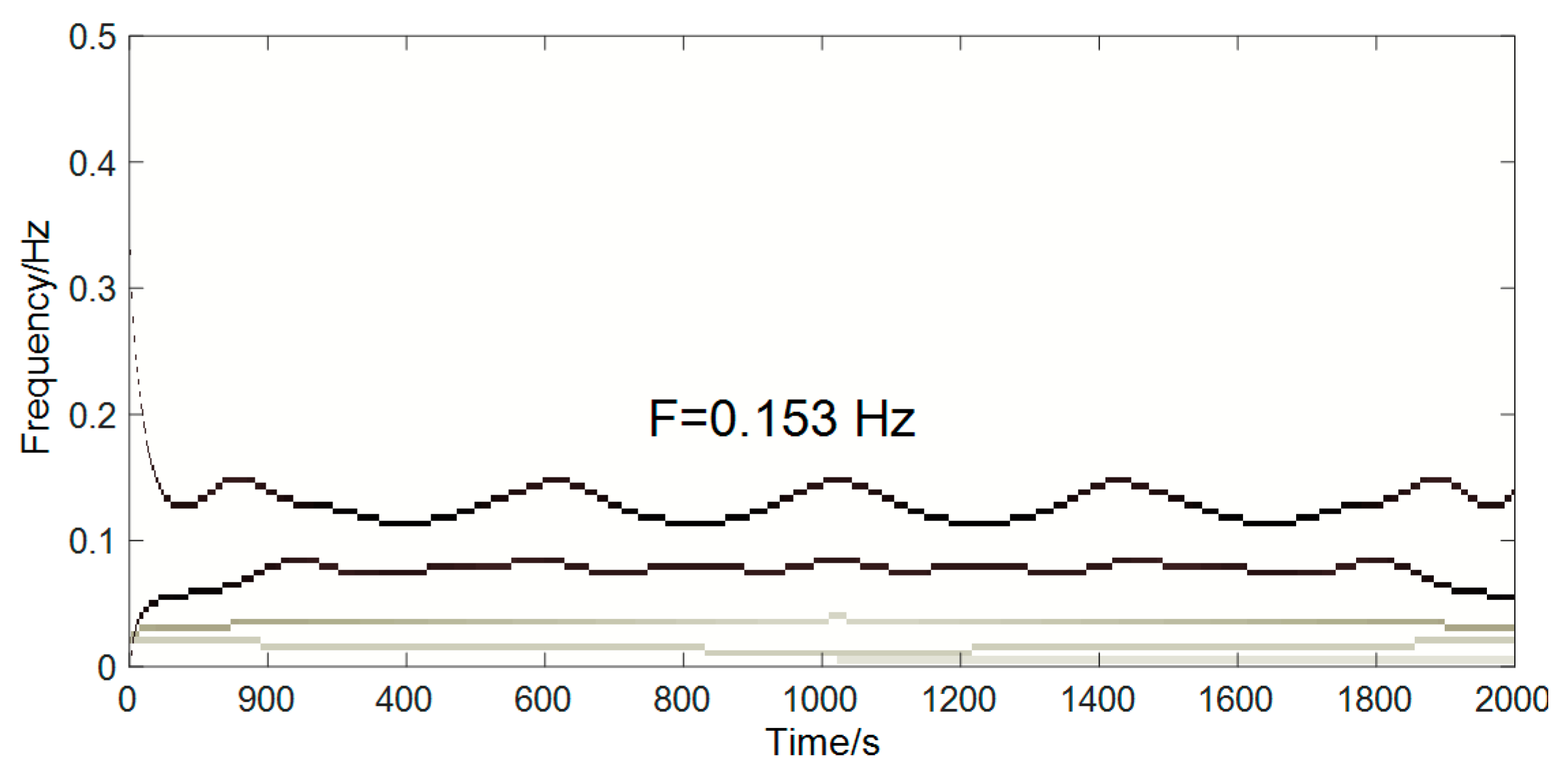
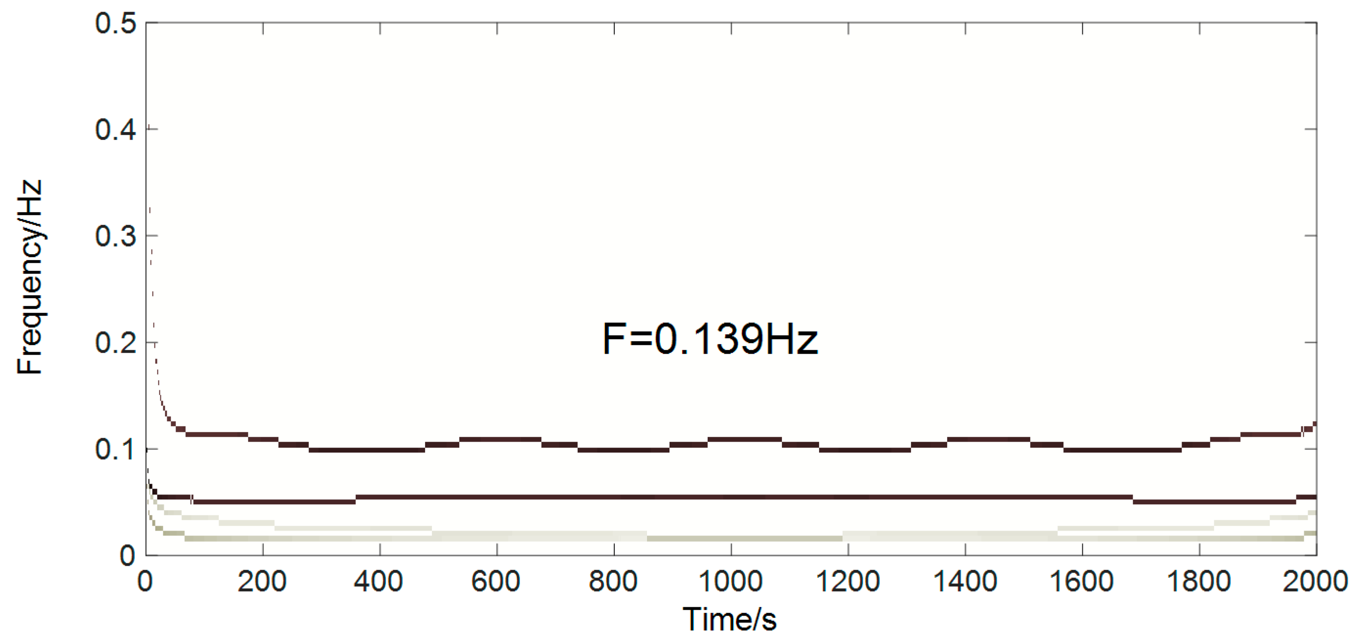
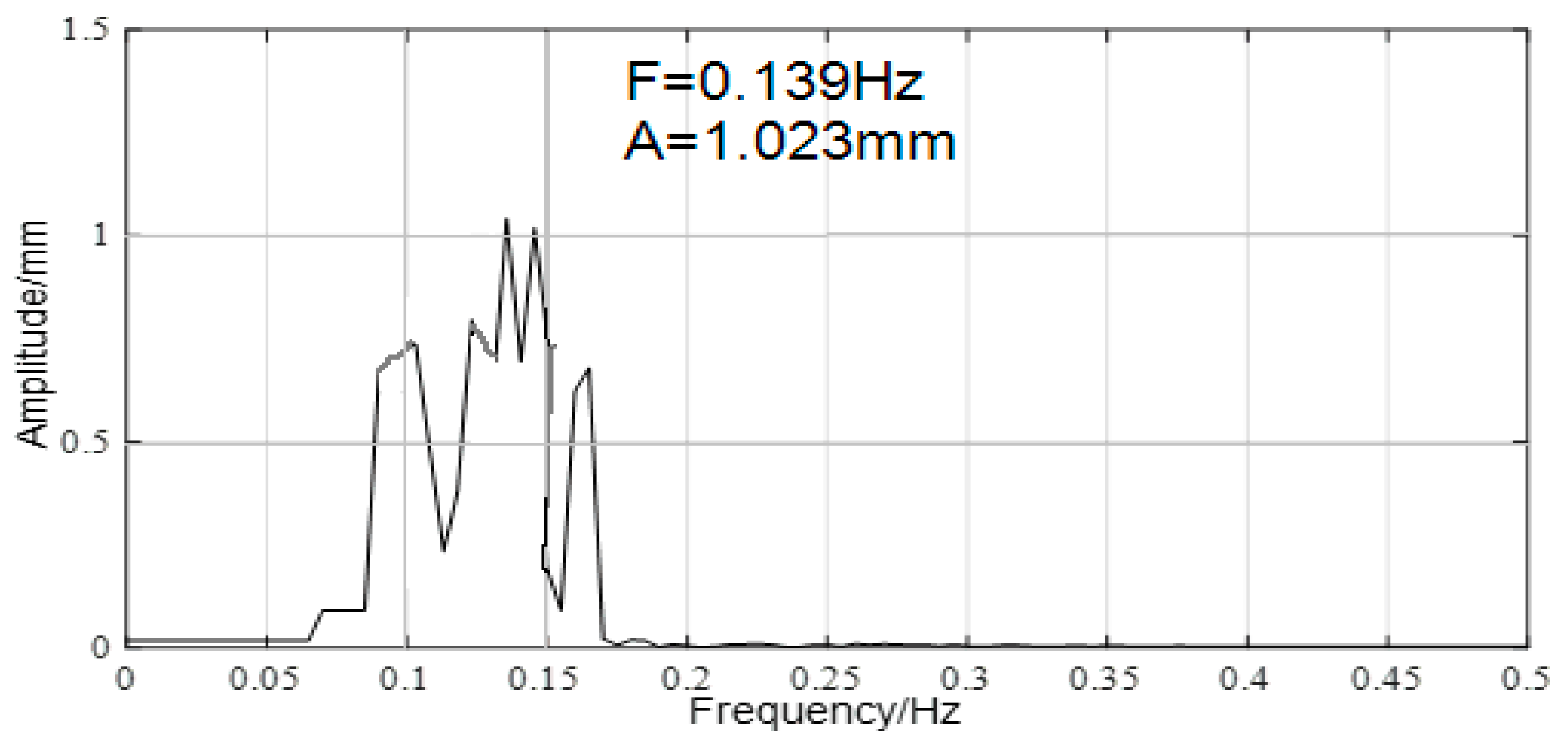
The Hilbert time spectrum and the marginal spectrum of the bridge structure were obtained via Hilbert spectral transformation from the reconstructed vibration components and are shown in Figure 15 and Figure 16, respectively. The results proved that the Hilbert marginal spectrum could accurately reflect the main frequency with the actual physical component. Similarly, multi-scale decomposition was performed on the observation data of the bridge in the vertical direction denoised by the wavelet-EMD method, and the correlation value was calculated. Then, the effective vibration components were selected for reconstruction. Finally, the Hilbert time spectrum and marginal spectrum of the bridge structure in the vertical direction were calculated and shown in Figure 17 and Figure 18, respectively.
Figure 15 and Figure 17 show the time-frequency spectrum of the vibration component of the bridge structure in the horizontal and vertical directions, respectively. A clear line existed between 0 and 0.2 Hz in each figure, and the maximum dominant frequencies were 0.153 and 0.139 Hz, respectively. Figure 16 and Figure 18 show the marginal spectrum of the vibration component of the bridge structure in the horizontal and vertical directions, respectively. An amplitude extremum existed in each marginal spectrum image, and 0.153 and 0.139 Hz corresponded to the two main frequency lines in Figure 15 and Figure 17, respectively. Comparison and analysis of the four graphs indicated that the vibration frequencies of the bridge in the horizontal and vertical directions were 0.153 and 0.139 Hz, respectively.
However, the reliability and precision of the first natural frequency identification results based on time-frequency analysis methods are often difficult to ensure in practical applications. The parameter values identified in this study must be compared with those of other different methods. The theoretical calculation value of the bending natural vibration frequency of Sutong Bridge in the horizontal direction was 0.145 Hz according to the theoretical and empirical calculation methods of the dynamic characteristics of long-span bridges [34,35,36], and the value of the vertical direction was 0.133 Hz. A comparison of the identification results with the theoretical calculations showed that the relative errors of the bridge structure in horizontal and vertical directions were 5.52% and 4.67%, respectively, and the statistical results are shown in Table 4.
Table 4 shows that the amplitude of the main frequency of the bridge in the horizontal direction (4.50 mm) was significantly larger than that in the longitudinal direction (1.02 mm), and the main frequency in the vertical direction of the bridge was not as prominent as the horizontal one. This result indicated that under environment excitation conditions, the loads, such as the construction environment and wind, exerted a larger influence on the longitudinal direction of the bridge. Similarly, analysis of the observation data from the monitoring points in other periods indicated that the first natural frequency was the same in horizontal and vertical directions, except for a slight difference in amplitude. This result indicated that the wavelet-EMD method was used to denoise the original observation data firstly. Then, Hilbert spectrum analysis was performed on the denoised data to obtain the accurate first natural frequency of the bridge structure. This scheme had high identification accuracy and could be used for dynamic characteristic extraction of bridge structures.
5. Conclusions
With the GNSS dynamic monitoring data of Sutong Bridge as the study object and in consideration of the low precision of first natural frequency identification due to noise interference caused by HHT processing of non-stationary signals, this study proposed a time-frequency analysis method based on the combination of wavelet threshold denoising and HHT. This method was applied to the analysis of the dynamic characteristics of a bridge structure. The conclusions were as follows:
- (1)
- The proposed wavelet-EMD method suppressed high-frequency noise effectively, decreased the decomposition layers of EMD, and reduced the margin effects on the quality of effective signal decomposition. The SNR and linear correlation coefficient of the denoised signal were the largest, and RMSE was the smallest. The method had a stable denoising effect in the horizontal and vertical directions.
- (2)
- The Hilbert spectrum analysis of the denoised data clearly reflected the spectral value of the bridge structure, and the numerical results agreed well with the theoretical calculations. The relative errors of the natural frequency identification in the horizontal and vertical directions were 5.52% and 4.67%, respectively, which meant that the natural vibration characteristics of the bridge structure were identified effectively.
Author Contributions
X.W. and S.H. participated in the design of this study, and they both performed the statistical analysis. X.W. carried out the study and collected important background information. X.W. and S.H. carried out the concepts, the design of data acquisition, the definition of the new algorithm, the literature search, the data analysis, and the manuscript preparation. X.W., C.K., G.L., and C.L. carried out the data acquisition, the literature search, and the manuscript editing. S.H., X.W., C.K., and C.L. performed the manuscript review. All authors read and approved the content of the manuscript.
Funding
This paper was supported by the National Natural Science Foundation of China under Grant 41274020 and also by Henan Polytechnic University’s Key Laboratory of Mine Spatial Information Technologies of National Administration of Surveying, Mapping and Geo-information of China under Grant KLM201806.
Acknowledgments
The authors would like to thank the National Natural Science Foundation of China and Henan Polytechnic University’s Key Laboratory of Mine Spatial Information Technologies of National Administration of Surveying, Mapping and Geo-information of China for the financial support.
Conflicts of Interest
The authors declare that they have no conflicts of interest.
Availability of Data and Materials
The data contained in this manuscript were the result of experiments by the research group. Data sharing is not applicable to this article as no datasets were generated or analyzed during the current study. Please contact the authors for data requests.
Abbreviations
| HHT | Hilbert–Huang transform |
| EMD | Empirical mode decomposition |
| wavelet-EMD | Wavelet-empirical mode decomposition |
| IMF | Intrinsic modal component |
| GNSS | Global Navigation Satellite System |
| HT | Hilbert transform |
References
- An, Y.H.; Chatzi, E.; Sim, S.H.; Laflamme, S.; Blachowski, B.; Ou, J.P. Recent progress and future trends on damage identification methods for bridge structures. Struct. Control. Health Monit. 2019, 26, e2416. [Google Scholar] [CrossRef]
- Xu, J.; Wang, Z.B.; Tan, C.; Si, L.; Zhang, L.; Liu, X.H. Adaptive Wavelet Threshold Denoising Method for Machinery Sound Based on Improved Fruit Fly Optimization Algorithm. Appl. Sci. 2016, 6, 199. [Google Scholar] [CrossRef] [Green Version]
- Khatir, S.; Belaidi, I.; Khatir, T.; Hamrani, A.; Zhou, Y.L.; Wahab, M.A. Multiple damage detection in unidirectional graphite-epoxy composite beams using particle swarm optimization and genetic algorithm. Mechanika 2017, 23, 514–521. [Google Scholar]
- Khatir, S.; Brahim, B.; Capozucca, R.; Wahab, M.A. Damage detection in CFRP composite beams based on vibration analysis using proper orthogonal decomposition method with radial basis functions and cuckoo search algorithm. Compos. Struct. 2018, 187, 344–353. [Google Scholar]
- Sheng, G.R.; Gao, G.W.; Zhang, B.Y. Application of Improved Wavelet Thresholding Method and an RBF Network in the Error Compensating of an MEMS Gyroscope. Micromachines 2019, 10, 608. [Google Scholar] [CrossRef] [PubMed] [Green Version]
- Khatir, S.; Wahab, M.A.; Djilali, B.; Khatir, T. Structural health monitoring using modal strain energy damage indicator coupled with teaching-learning-based optimization algorithm and isogoemetric analysis. J. Sound Vib. 2019, 448, 230–246. [Google Scholar] [CrossRef]
- Tran-Ngoc, H.; He, L.Q.; Reynders, E.; Khatir, S.; Le-Xuan, T.; Roeck, G.D.; Bui-Tien, T.; Wahab, M.A. An efficient approach to model updating for a multispan railway bridge using orthogonal diagonalization combined with improved particle swarm optimization. J. Sound Vib. 2020, 476, 115315. [Google Scholar] [CrossRef]
- Wang, G.H.; Liu, Q.; Wang, C.Z.; Dong, L.L.; Dai, D.; Shen, L. Study of Blockage Diagnosis for Hydrocyclone Using Vibration-Based Technique Based on Wavelet Denoising and Discrete-Time Fourier Transform Method. Processes 2020, 8, 440. [Google Scholar] [CrossRef] [Green Version]
- Yu, J.Y.; Meng, X.L.; Yan, B.F.; Xu, B.; Fan, Q.; Xie, Y.L. Global Navigation Satellite System-based positioning technology for structural health monitoring: A review. Struct. Control. Health Monit. 2020, 27, e2467. [Google Scholar] [CrossRef] [Green Version]
- Guo, J.; Xu, L.; Dai, L.; Mcdonald, M.; Wu, J.; Li, Y. Application of the Real-Time Kinematic Global Positioning System in Bridge Safety Monitoring. J. Bridge. Eng. 2005, 3, 163–168. [Google Scholar] [CrossRef]
- Huang, S.X.; Wang, X.P.; Li, C.F.; Kang, C. Data decomposition method combining permutation entropy and spectral substitution with ensemble empirical mode decomposition. Measurement 2019, 139, 438–453. [Google Scholar] [CrossRef]
- Ogundipe, O.; Lee, J.K.; Roberts, G.W. Wavelet De-noising of GNSS Based Bridge Health Monitoring Data. J. Appl. Geod. 2014, 8, 273–281. [Google Scholar] [CrossRef]
- Mousavi, A.A.; Zhang, C.W.; Masri, S.F.; Gholipour, G. Structural Damage Localization and Quantification Based on a CEEMDAN Hilbert Transform Neural Network Approach: A Model Steel Truss Bridge Case Study. Sensors 2020, 20, 1271. [Google Scholar] [CrossRef] [PubMed] [Green Version]
- Nakamura, S.P.E. GPS measurement of wind-induced suspension bridge girder displacements. J. Struct. Eng. 2000, 10, 1413–1419. [Google Scholar] [CrossRef]
- Mosbeh, R.; Kaloop, M.; Li, H. Monitoring of Bridge Deformation Using GPS Technique. J. Civ. Eng. 2009, 13, 423–431. [Google Scholar]
- Yang, S.X.H.B.C.; Zhang, H.; Mei, W.S. Real-time Dynamic Monitoring with GPS and Georobot During Sutong Bridge Construction. Acta Geod. Et Cartogr. Sin. 2009, 38, 66–72. [Google Scholar]
- Huang, S.X.; Luo, L.; He, C. Comparative Test Analysis for Determining Bridge Deflection by Using Ground-Based SAR and GPS. Geomat. Inf. Sci. Wuhan Univ. 2012, 37, 1173–1176. [Google Scholar]
- Han, H.; Wang, J.; Meng, X.; Liu, H. Analysis of the dynamic response of a long span bridge using GPS/accelerometer/anemometer under typhoon loading. Eng. Struct. 2016, 122, 238–250. [Google Scholar] [CrossRef]
- Kaloop, M.R.; Kim, D. GPS-structural health monitoring of a long span bridge using neural network adaptive filter. Surv. Rev. 2014, 46, 7–14. [Google Scholar] [CrossRef]
- Dai, W.J.; Huang, D.W.; Cai, C.S. Multipath mitigation via component analysis methods or GPS dynamic deformation monitoring. GPS Solut. 2014, 18, 417–428. [Google Scholar] [CrossRef]
- Li, X.; Li, Z.; Wang, E.; Feng, J.; Chen, L.; Li, N.; Kong, X. Extraction of microseismic waveforms characteristics prior to rock burst using Hilbert–Huang transform. Measurement 2016, 91, 101–113. [Google Scholar] [CrossRef]
- Huang, S.X.; Liu, J.N.; Liu, X.L. Deformation Analysis Based on Wavelet and Its Applicationin Dynamic Monitoring for High-rise Buildings. Acta Geod. Et Cartogr. Sin. 2003, 32, 153–157. [Google Scholar]
- Yan, K.; Ni, Z.; Zhang, H.; Guo, W.; Niu, X.; Liu, J. Weak GPS signal tracking using FFT discriminator in open loop receive. GPS Solut. 2016, 20, 225–237. [Google Scholar] [CrossRef]
- Ragheb, A.E.; Edwards, S.J.; Clarke, P.J. Using Filtered and Semi-continuous High Rate GPS for Monitoring Deformations. J. Surv. Eng. 2010, 136, 72–79. [Google Scholar] [CrossRef] [Green Version]
- Xiao, Y.; Feng, C.J. A Time-frequency Representation Method of STFT with Combining Window Functions. J. Detect. Control. 2010, 45–49. (In Chinese) [Google Scholar]
- Huang, N.; Shen, Z.; Long, S.R.; Wu, M.C.; Shih, H.H.; Zheng, Q.; Yen, N.-C.; Tung, C.C.; Liu, H.H. The empirical mode decomposition and the Hilbert spectrum for nonlinear and non-stationary time series analysis. Proc. R. Soc. Lond. Ser. A Math. Phys. Eng. Sci. 1998, 454, 903–995. [Google Scholar] [CrossRef]
- Yu, J.T.; Zhao, S.Y.; Wang, Q. De-nosing of acoustic emission signals based on empirical mode decomposition and wavelet transform. J. Harbin Inst. Technol. 2011, 43, 88–92. [Google Scholar]
- Luo, F.X.; Dai, W.J.; Tang, C.J.; Huang, D.W.; Wu, X.X. EMD-ICA with reference signal method and its application in GPS multipath. Acta Geod. Et Cartogr. Sin. 2012, 41, 366–371. [Google Scholar]
- Xu, J.; Huang, S.X.; Ma, F.H. The Dynamic Characteristics Analysis for the Large Bridge Based on the Improved Hilbert-Huang Transformation. Geomat. Inf. Sci. Wuhan Univ. 2010, 35, 801–805. [Google Scholar]
- Wu, Z.; Huang, N. Ensemble empirical mode decomposition: A noise-assisted data analysis method. Adv. Adapt. Data Anal. 2009, 1, 1–41. [Google Scholar] [CrossRef]
- Zheng, J.; Cheng, J.; Yang, Y. Partly ensemble empirical mode decomposition: An improved noise-assisted method for eliminating mode mixing. Signal. Process. 2014, 96, 362–374. [Google Scholar] [CrossRef]
- Zhang, W.W. Neighboring adaptive Bayes Shrink image denoising in dual-tree complex wavelet transform. Comput. Eng. Appl. 2012, 48, 156–160. [Google Scholar]
- Zhu, Y.G.; Yang, X.L. A Dyadic Wavelet Filtering Method for 2-D Image Denoising. J. Signal Inf. Process. 2011, 2, 308–315. [Google Scholar] [CrossRef] [Green Version]
- He, M.X.; Yang, B.C.; Huang, S.X.; You, X.P.; Tian, W. Analysis and Research of the Dynamic Characteristics of Large Cable-stayed Bridge During Construction. J. Wuhan Univ. Technol. (Transp. Sci. Eng.) 2011, 35, 516–519. [Google Scholar]
- Xu, F.Y.; Chen, A.R. 3-D flutter analysis of Sutong bridge. Eng. Mech. 2008, 25, 139–144. (In Chinese) [Google Scholar]
- Mao, J.X.; Wang, H.; Xun, Z.X. Comparison Study on Modal Parameter Identification of Large Span Cable Stayed Bridge with Time-frequency Method. J. Tongji Univ. (Nat. Sci.) 2016, 44, 996–1001. (In Chinese) [Google Scholar]
Figure 1.
Flowchart of the HHT algorithm.

Figure 2.
Flowchart of the wavelet-EMD denoising method.

Figure 3.
Waveforms of the simulation signals containing noise.

Figure 4.
Results of wavelet denoising (the original signal SNR: 4dB).

Figure 5.
Results of EMD denoising (the original signal SNR: 4dB).

Figure 6.
Results of wavelet-EMD denoising (the original signal SNR: 4dB).
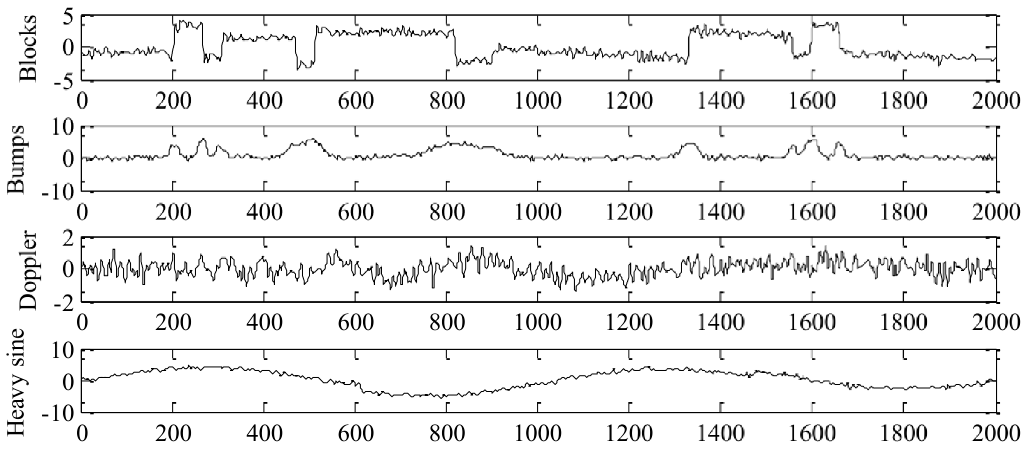
Figure 7.
Layout of the GNSS monitoring points on Sutong Bridge.
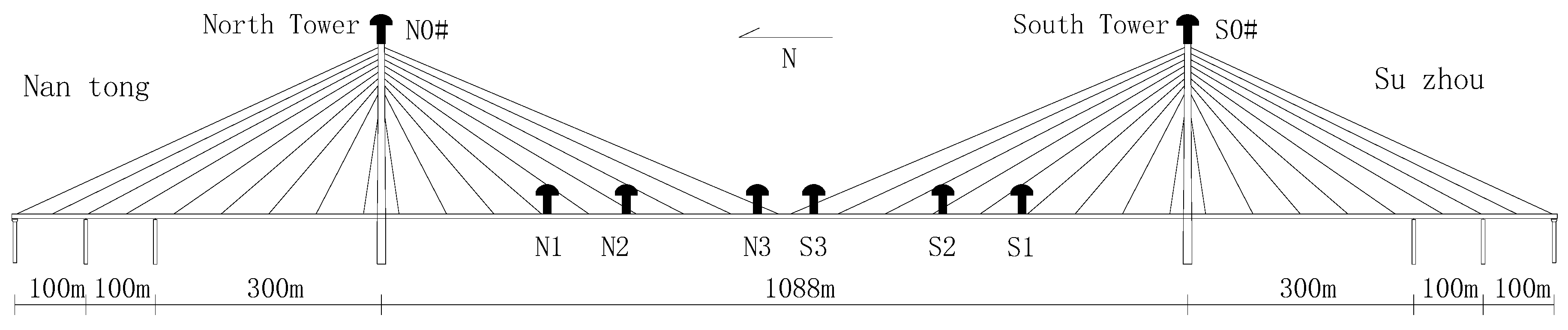
Figure 8.
Time series diagram of the original observation data.

Figure 9.
Comparison of denoising results from four methods in the time domain: (a) horizontal direction and (b) vertical direction. H-Wavelet represents hard threshold denoising, S-Wavelet represents soft threshold denoising, I-Wavelet represents half threshold denoising, and WE represents wavelet-EMD denoising
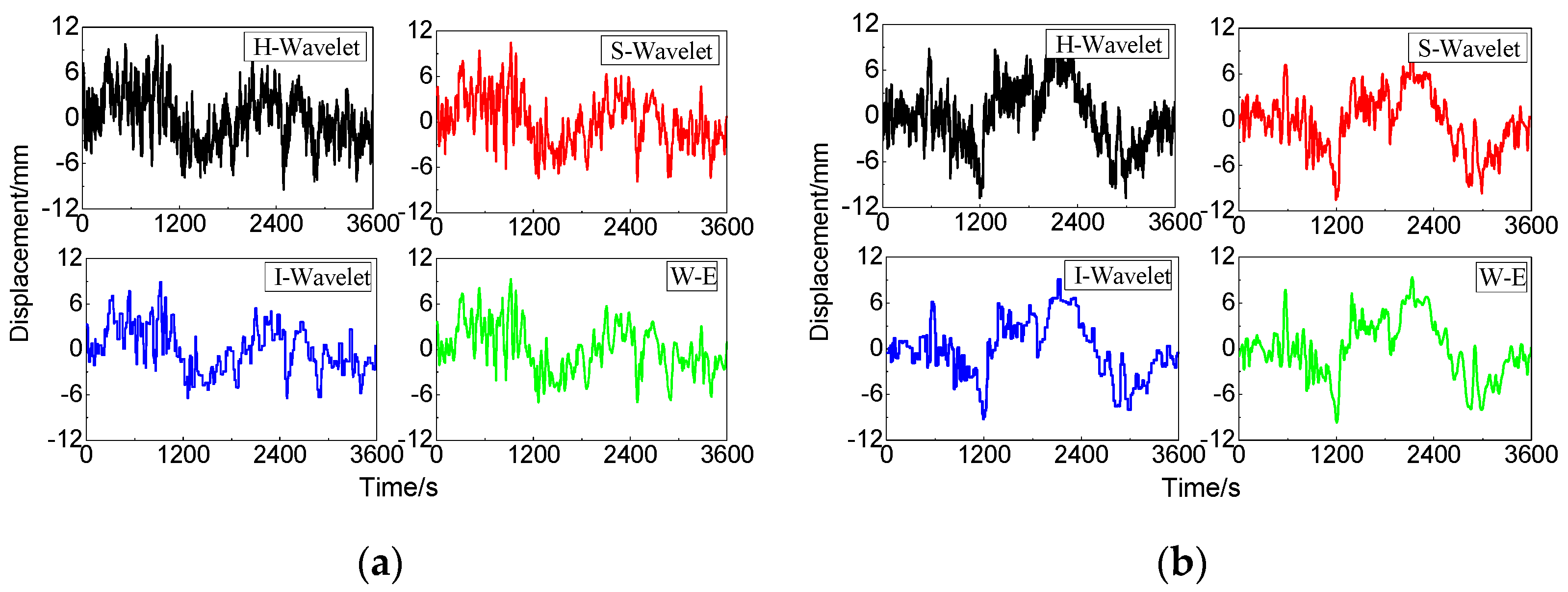
Figure 10.
Comparison of denoising results from the four methods in the frequency domain: (a) horizontal direction and (b) vertical direction.
Figure 10.
Comparison of denoising results from the four methods in the frequency domain: (a) horizontal direction and (b) vertical direction.

Figure 11.
Decomposition result of the noisy observation sequence in the horizontal direction using EMD.
Figure 11.
Decomposition result of the noisy observation sequence in the horizontal direction using EMD.
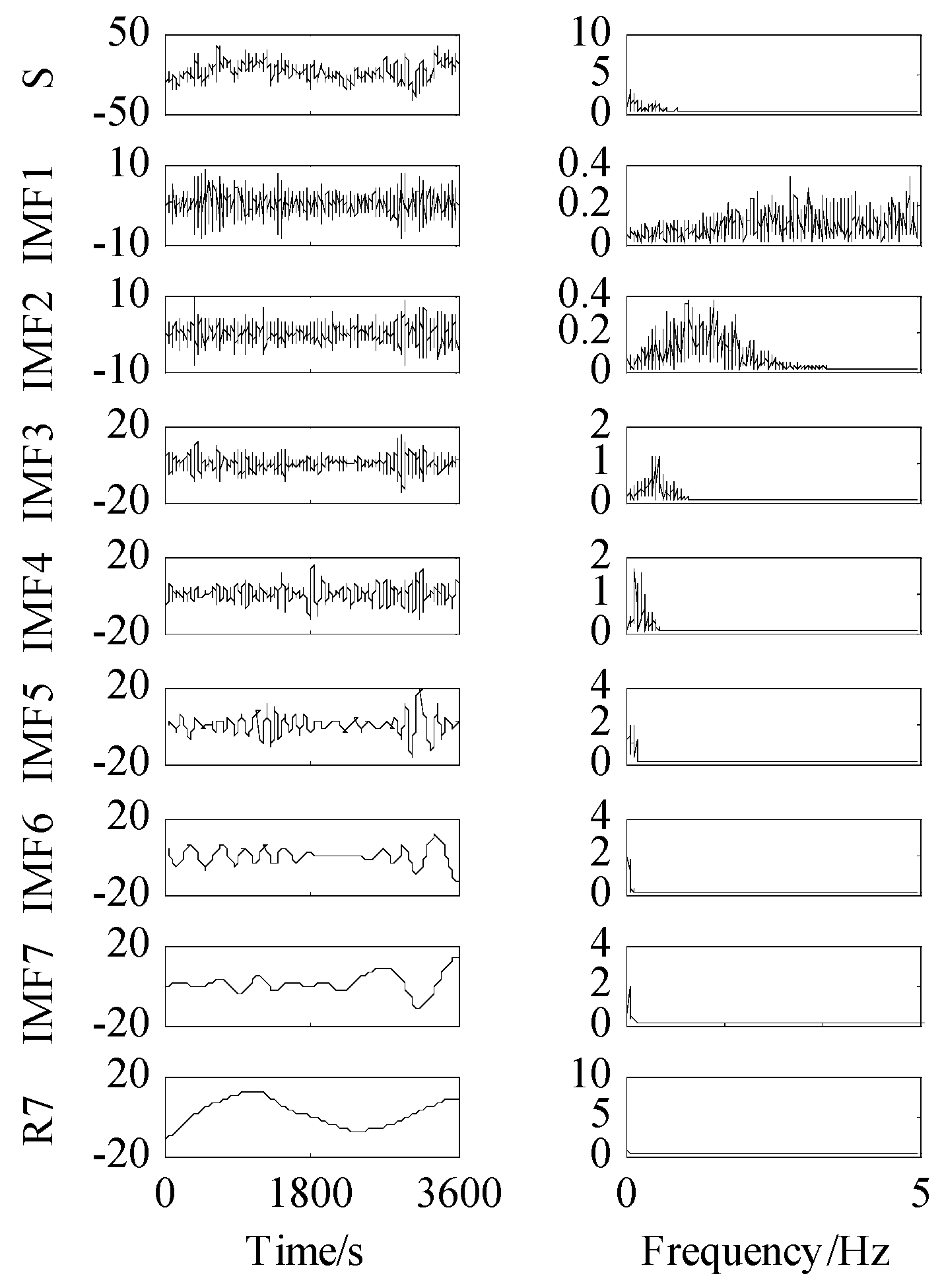
Figure 12.
Decomposition result of the denoised signal in the horizontal direction using EMD.

Figure 13.
Correlation values of respective IMF components from the noisy observation sequence.

Figure 14.
Correlation values of respective IMF components from the denoised signal.
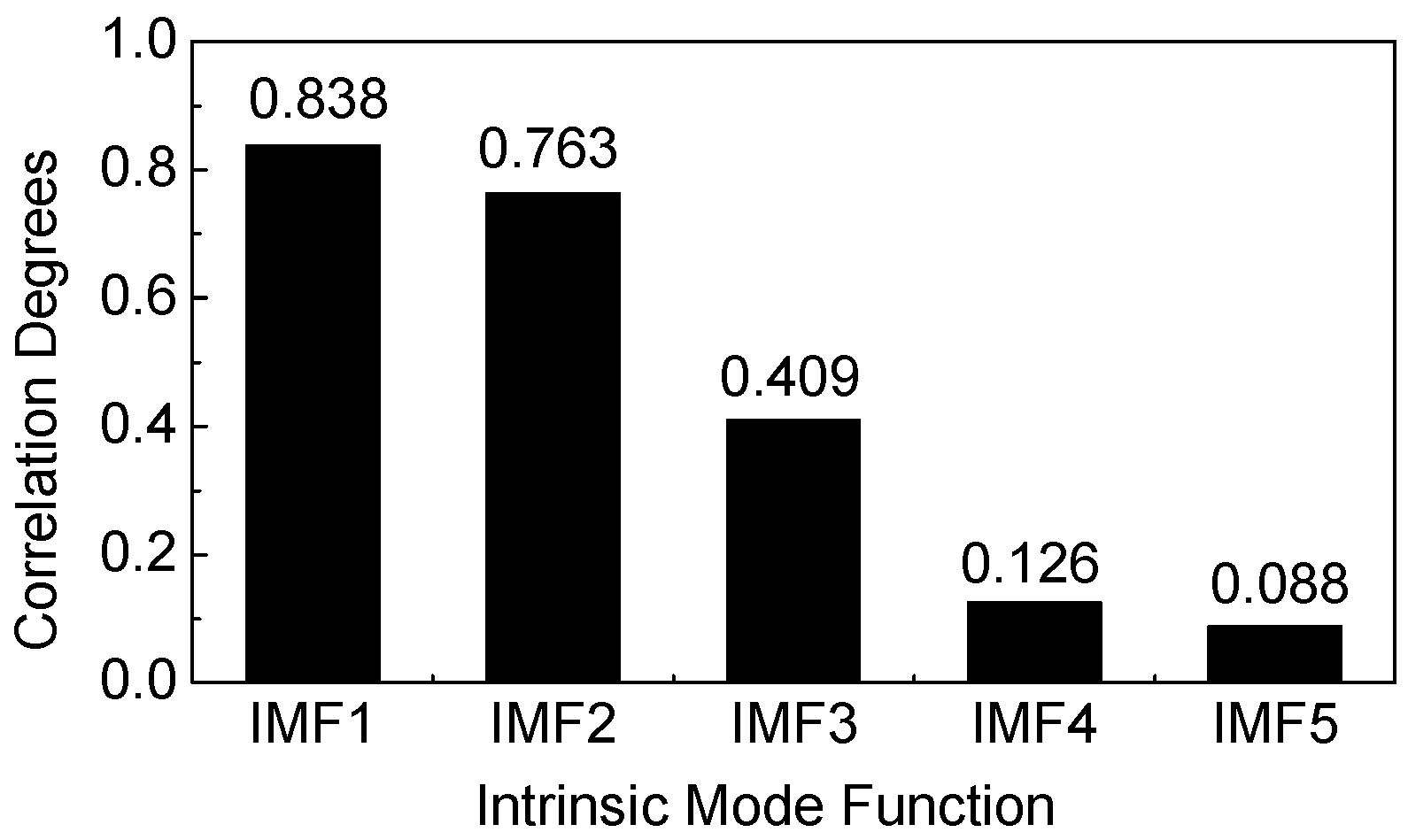
Figure 15.
Hilbert time spectrum of the denoised observation sequence in the horizontal direction.

Figure 16.
Hilbert marginal spectrum of the denoised observation sequence in the horizontal direction.
Figure 16.
Hilbert marginal spectrum of the denoised observation sequence in the horizontal direction.
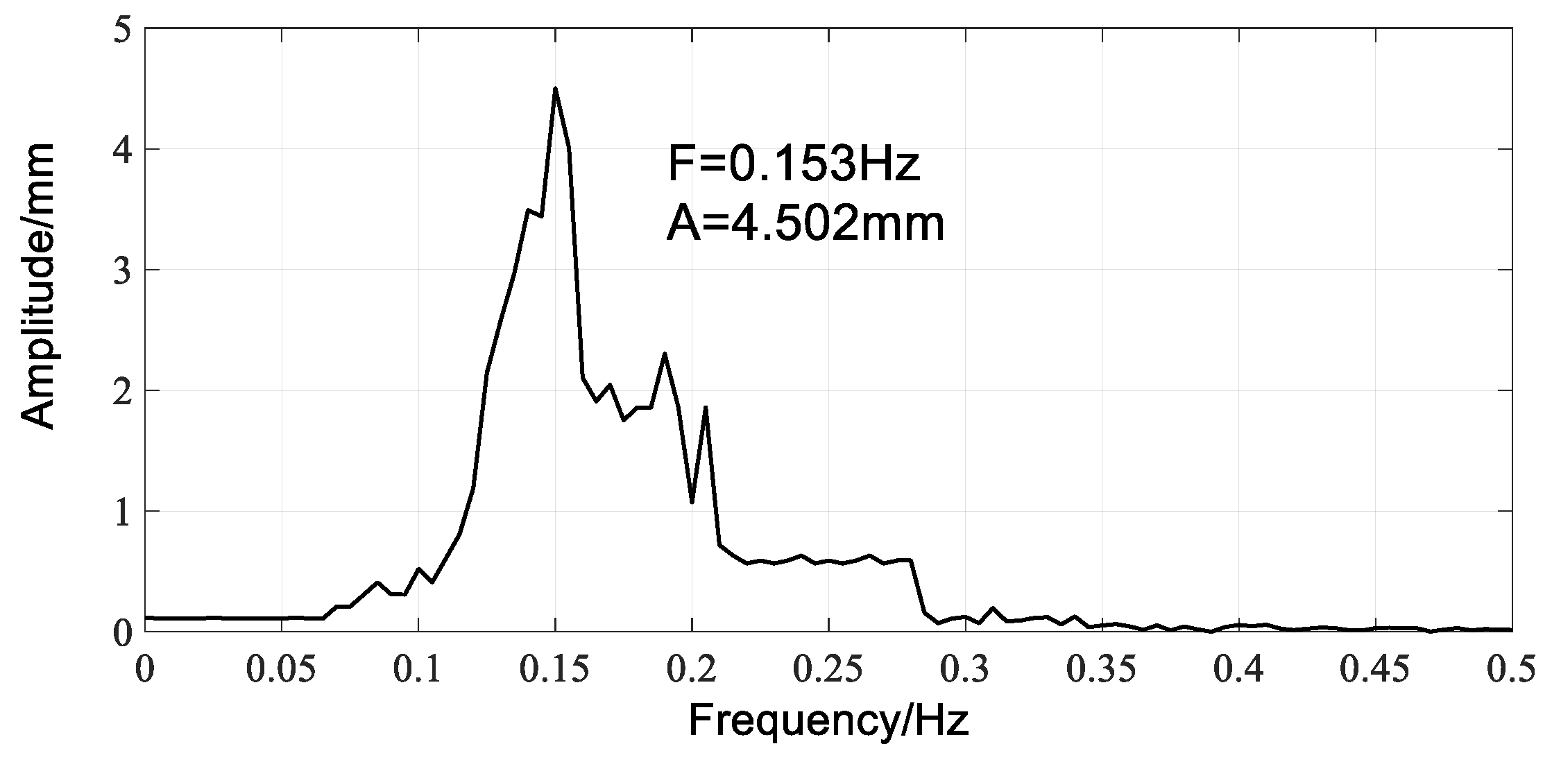
Figure 17.
Hilbert time spectrum of the denoised observation sequence in the vertical direction.

Figure 18.
Hilbert marginal spectrum of the denoised observation sequence in the vertical direction.
Figure 18.
Hilbert marginal spectrum of the denoised observation sequence in the vertical direction.


Table 1.
Denoising results from the different methods.
| Denoising Methods | Blocks Signal | Bumps Signal | Doppler Signal | Heavy Signal | ||||
|---|---|---|---|---|---|---|---|---|
| SNR | RMSE | SNR | RMSE | SNR | RMSE | SNR | RMSE | |
| Noisy signal | 11.593 | - | 8.855 | - | 7.403 | - | 6.357 | - |
| Wavelet denoising | 20.035 | 0.855 | 15.872 | 0.455 | 15.896 | 0.354 | 14.156 | 0.558 |
| EMD denoising | 21.065 | 0.413 | 16.828 | 0.448 | 14.017 | 0.417 | 15.384 | 0.491 |
| Wavelet-EMD | 21.428 | 0.362 | 18.147 | 0.362 | 20.548 | 0.252 | 19.285 | 0.328 |
Table 2.
Denoising results from the different methods on signals with different SNR.
| Signal SNR | Denoising Methods | Blocks Signal | Bumps Signal | Doppler Signal | Heavy Signal | ||||
|---|---|---|---|---|---|---|---|---|---|
| SNR | RMSE | SNR | RMSE | SNR | RMSE | SNR | RMSE | ||
| 6 dB | Noisy signal | 15.573 | - | 15.467 | - | 13.403 | - | 12.357 | - |
| Wavelet denoising | 19.038 | 0.578 | 16.872 | 0.655 | 15.896 | 0.454 | 14.156 | 0.558 | |
| EMD denoising | 21.372 | 0.316 | 17.538 | 0.888 | 16.017 | 0.316 | 15.354 | 0.491 | |
| Wavelet-EMD | 20.819 | 0.376 | 18.147 | 0.369 | 17.643 | 0.202 | 16.069 | 0.343 | |
| 2 dB | Noisy signal | 6.593 | - | 5.855 | - | 4.403 | - | 4.357 | - |
| Wavelet denoising | 11.168 | 0.555 | 10.364 | 0.462 | 9.764 | 0.409 | 9.156 | 0.306 | |
| EMD denoising | 12.083 | 0.413 | 10.905 | 0.491 | 10.375 | 0.438 | 7.874 | 0.492 | |
| Wavelet-EMD | 13.575 | 0.362 | 12.643 | 0.359 | 12.871 | 0.252 | 9.018 | 0.330 | |
| −2 dB | Noisy signal | −2.451 | - | −3.855 | - | −4.313 | - | −5.357 | - |
| Wavelet denoising | 5.035 | 0.455 | 6.872 | 0.563 | 6.831 | 0.684 | 3.876 | 0.678 | |
| EMD denoising | 6.362 | 0.417 | 5.828 | 0.431 | 7.707 | 0.586 | 4.321 | 0.529 | |
| Wavelet-EMD | 7.352 | 0.335 | 8.847 | 0.369 | 9.353 | 0.309 | 6.963 | 0.338 | |
Table 3.
Results of the four denoising methods in the horizontal and vertical directions.
| Denoising Methods | Horizontal Direction | Vertical Direction | ||||
|---|---|---|---|---|---|---|
| SNR | RMSE (mm) | R | SNR | RMSE (mm) | R | |
| H-Wavelet | 8.434 | 3.609 | 0.938 | 8.704 | 0.689 | 0.928 |
| S-Wavelet | 8.856 | 3.019 | 0.951 | 8.387 | 0.784 | 0.920 |
| I-Wavelet | 10.082 | 2.169 | 0.962 | 9.186 | 0.369 | 0.953 |
| Wavelet-EMD | 11.134 | 1.904 | 0.971 | 10.246 | 0.365 | 0.965 |
Table 4.
Horizontal and vertical frequencies of the bridge structure and its amplitude.
| Direction | Measured Frequency (Hz) | Theoretical Calculation (Hz) | Relative Error (%) | Amplitude (mm) |
|---|---|---|---|---|
| Horizontal | 0.153 | 0.145 | 5.52 | 4.50 |
| Vertical | 0.139 | 0.133 | 4.67 | 1.02 |
© 2020 by the authors. Licensee MDPI, Basel, Switzerland. This article is an open access article distributed under the terms and conditions of the Creative Commons Attribution (CC BY) license (http://creativecommons.org/licenses/by/4.0/).
Share and Cite
MDPI and ACS Style
Wang, X.; Huang, S.; Kang, C.; Li, G.; Li, C. Integration of Wavelet Denoising and HHT Applied to the Analysis of Bridge Dynamic Characteristics. Appl. Sci. 2020, 10, 3605. https://doi.org/10.3390/app10103605
AMA Style
Wang X, Huang S, Kang C, Li G, Li C. Integration of Wavelet Denoising and HHT Applied to the Analysis of Bridge Dynamic Characteristics. Applied Sciences. 2020; 10(10):3605. https://doi.org/10.3390/app10103605
Chicago/Turabian StyleWang, Xinpeng, Shengxiang Huang, Chao Kang, Guanqing Li, and Chenfeng Li. 2020. "Integration of Wavelet Denoising and HHT Applied to the Analysis of Bridge Dynamic Characteristics" Applied Sciences 10, no. 10: 3605. https://doi.org/10.3390/app10103605
Note that from the first issue of 2016, this journal uses article numbers instead of page numbers. See further details here.