Self-Adaptation of a Heterogeneous Swarm of Mobile Robots to a Covered Area

Abstract

An original swarm-based method for coordination of groups of mobile robots with a focus on the self-organization and self-adaptation of the groups is presented in this paper. The method is a nature-inspired decentralized algorithm that uses artificial pheromone marks and enables the cooperation of different types of independent reactive agents that operate in the air, on the ground, or in the water. The advantages of our solution include scalability, adaptability, and robustness. The algorithm worked with variable numbers of agents in the groups. It was resistant against failures of the individual robots. A transportation control algorithm that ensured the spreading of different types of agents across exploration space with different types of environments was introduced and tested. We established that our swarm control algorithm was able to successfully control three basic behaviors: space exploration, population management, and transportation. The behaviors were able to run simultaneously, and space exploration (the main goal) was never stopped or interrupted. All these features combined in a single algorithmic package represent a framework for future development of swarm-based agent systems applicable in a broad scope of environments. The results confirmed that the algorithm can be applied to monitoring, surveillance, patrolling, or search and rescue tasks.

1. Introduction and Related Works

The availability of cheap mobile robots that can be deployed in large quantities has dramatically increased over the last decade. Robust and scalable algorithms are needed to control large groups of robots. The field of swarm robotics studies the coordination of large groups of relatively simple robots using simple local rules. It is inspired by the behavior of social insects that can accomplish tasks that are beyond the capabilities of any individual (see, e.g., in [1,2,3]). Iocchi et al. presented a taxonomy of swarm robotic systems structured into several levels in [4]. According to this taxonomy, swarm robotic systems are cooperative, aware, strongly coordinated or weakly coordinated, and distributed. Inaki and Matía summarized the basic behaviors and tasks solved in swarm robotics in [5] aggregation, dispersion, pattern formation, collective movement, task allocation, source search, the collective transport of objects, and collective mapping. Swarm robot behaviors can be categorized according to spatially distributed multi-robot movements [6].

Although there are some works dealing with heterogenous agent swarms [7], most of the algorithms operate with robots, which are of single type; therefore, the group or swarm is homogeneous and operates in a single environment with faultless communication channels. The ambition of the study is to create a unified algorithm, which will be able to operate in a set of environments using a custom swarm strategy to solve the coverage problem even with limited communication. The space to be covered is divided into cells and solving the coverage problem means visiting each cell by a robot at least once. Contrary to traditional approaches in swarm robotics and their control algorithms, we assume that the space to be covered comprises different environments, that the robots are of different types, and that each robot type has different capabilities. Covering an unfamiliar space is difficult and usually not solved by other algorithms, especially if the environment is dynamic. We also assume that the trajectories of the individual robots should not be easily predictable. Difficult predictability for the robots’ trajectories is greatly advantageous for applications, such as patrolling. A combination of all these features in a single framework algorithm is a very perspective and novel approach, so far not published or developed in the known literature. The aim of the study is to prove that such algorithm can be designed and is able to explore different environments in finite time.

A large body of research has investigated robot or multi-robot coverage and exploration problems. Many experimental and real life applications have been implemented in 2D [8,9,10], 2.5D [11,12,13], and 3D [14,15] environments. Applications of the coverage path planning in domains, such as agricultural robotics [16] and unmanned aerial vehicles (UAVs) [11,17,18,19], have also been described. Another approach that could be pointed out here is the centralized vs. the decentralized mode of the swarm with negotiation process applied to a survey task [7,20]. The negotiation process enables each robot to find the best solution by reassigning subtasks through the process of finding the utility value of the specific sub-task. This solution used the Robot Utility Based Task Assignment (RUTA) algorithm. While in the case of decentralized control the robots broadcast their utility values for the sub-tasks and the best robots are selected [7], our solution use only the pheromone value to control all processes. A more comprehensive description and explanation of the existing methods together with a detailed classification of the existing approaches is given in [21]. It can be said that many approaches deal with the optimal space coverage methods.

Senthilkumar and Bharadwaj used a spanning tree coverage algorithm for optimal 2D space exploration in [10]. Another interesting approach to the foraging problem was solved in a robotic swarm using continually updated policies while drawing directions using simulated ant pheromones in [22]. These approaches used cellular automata as a platform and pheromone marks for coordination. Zelinsky et al. focused on the problem of complete coverage of an unstructured environment by a mobile robot solved with a deterministic algorithm in [23]. The optimization criterion in single-robot exploration is the overall exploration time minimization. In the case of using multiple robots for exploration, the main problem is setting the appropriate target points for the individual robots. Cao et al. [24] improved the path planning in 3D cellular space by a D* algorithm.

A review of various methods for solving the optimal coverage path for a defined swarm of robots and the efficiency of the methods is discussed in [25]. It is necessary to re-plan the individual paths in the case of a single robot malfunction. Several authors [2,3,26] combined optimization methods with virtual bird flocking. The multi-robot coverage problem in an unknown 2D space can also be solved using frontier-based techniques, such as Burgard et al. described in [27]; however, the authors did not investigate the expansion of their methods to 3D. Wagner et al., in [28], performed one of the first attempts to use an ant colony strategy using artificial pheromones to solve coverage problems and showed that the algorithm was adaptive and self-stabilizing.

Another algorithm based on pheromone marks is the the evaporation of a pheromone dropped by reactive agents (EVAP) algorithm, applied to the patrolling problem, that was introduced in [29]. The EVAP model can be considered to be an extension of the algorithm described in [30]. A variation of the ant colony optimization (ACO) algorithm called the chaotic ant colony optimization to coverage (CACOC) was explored in [31]. This approach integrates ACO with the chaotic dynamical system and can be employed in military surveillance. However, the UAV swarm still shares a virtual map to guide the motions of the vehicles.

The approaches described above were inspired by the behavior of social insects. The agents in the swarm, however, cannot adjust the size of the population themselves according to the size of their mission’s environment. Typically in swarm robotics, the authors use homogeneous groups of robots, i.e., the robots are of the same type. Modern trends combine robots of different types, for example, in outdoor environments [32]. The basic control functions of the robots are executed by the on-board computers. Many works address the problems of local control of mobile robots. The solutions are task- and robot-specific as, for example, in [33].

In this article, we focus on the self-adaptation of a population of a heterogeneous swarm (combined agents of different types and abilities) of mobile agents operating in a heterogeneous environment. The agents can be different types of robots like unmanned airplanes, copter drones, submarines, autonomous land vehicles, humanoid robots, or even software agents. The agents can have different sensor capabilities and are suitable for different environments. The proposed approach aims to be general enough to allow transportation of one agent type with another (e.g., a vehicle can transport a copter drone or vice versa). The novelty of the algorithm should also lie in the formalization of this concept. Therefore individual mobile agents do not need to know the attributes of the environments. They adapt themselves to the environment. Examples of hardware implementations of agents and overview of different approaches to their construction and capabilities can be found in [34].

The approach is fault-tolerant to the agent robot failure. It means that there is no need for any centralizer authority to manage/control other robots in case of a failure, which increases the robustness. The aim of this research was to create an algorithm that can operate in an environment without the need of an observer to predict the motion of the agents and operate without any a prior knowledge or knowledge of the actual state of the environment. Without the centralized control element and with the algorithm not being reliant on communication between agents as its design features, it can be expected that the algorithm will be robust in this regard. Not having the motion predictable but rather emergent due to using evaporating pheromone is a very important feature in a mission where deterministic algorithms perform stable and recognizable patterns (border guarding, area scanning, etc.) and is beneficial in the event of a communication failure. Another advantage of the pheromone marks control swarm strategy is the fact that each part of the explored space has a non-zero probability that it will be explored at any time during the exploration. This is an important feature that is different from deterministic algorithms where a cell has zero probability to be visited between two passes in the same exploration episode, [35]. Another advantage of our approach is its scalability and the ability of the algorithm to change swarm size according to environment type and size.

This paper is organized as follows. In Section 2, we recap our previous work and studies regarding pheromone-based swarm search technique. In Section 3, we present the definitions and descriptions of the basic constants of the proposed algorithm, and these are described in detail in Section 4. In Section 5, we present the simulation experiments, discussing the obtained results. In Section 6, we conclude the work and present the results in a broader scope of application possibilities and also expand the ideas for future work and improvements of the algorithm.

2. Previous Work and Study

It is very important to create robust control and coordination strategies to avoid and manage failures. Many control algorithms are fault tolerant but often at the cost of high complexity (e.g., complex rules of decision-making and the need for a higher authority). Our goal was to create a robust gracefully degrading multi-agent control system. Pheromone marks are commonly used to handle problems of coordination for a group of individuals (see, e.g., in [28,29,35]). However, in our case, we are trying to combine the concept of pheromone marks with population of heterogeneous agents and heterogeneous environment with transportable agents, which can be considered as a novel approach laying framework for future goal-oriented developments.

Initially, we implemented an algorithm that used artificial pheromone marks for the coordination of a group of robots [36]. We analyzed the properties of the algorithm in a 2D space (a similar work was described in [37]). We investigated the algorithm’s properties based on different sizes of swarms and various parameters of the pheromone mark’s evaporating times in [35]. We studied the influence of the evaporating time of the artificial pheromone marks on the exploration time. We also experimented with various swarm sizes. Our experiments showed that even in the case that all agents are broken except one, the single individual (agent) can complete the space exploration and monitoring tasks. We have proven the viability of our approach through outdoor tests (Short video from testing is available at https://youtu.be/OwG2u9FNtlU) [36]. We have used UAVs (quadcopters) based on the ardupilot platform, developed in our laboratory (http://www.ui.sav.sk/w/en/dep/mcdp/lab/). The algorithm was robust enough to manage the failures of the individual UAVs. Our agent-based solution used broadcast (The design of the real chemical pheromone liquid is challenging, from this reason, we used the broadcast communication in outdoor UAV testing.) communication to share the information of the simulated pheromone marks. Each agent broadcast a message with the information on new pheromone marks. We presented experiments with communication failures in [35]. We proved the fault tolerance and robustness of our method in this regard using outdoor tests [36].

We described the solution of the same problem in 3D space in [38]. We evaluated the performance improvement of the method in [39] and further elaborated the method in [38], where we reduced the number of conflicts (The conflict represents a situation when two or more agents want to move to the same position or their motion trajectory is being crossed.) by modifying the behavior of the individual agents. The measures taken to reduce the number of conflicts negatively affected the exploration ability of the swarm. However, the conflicts allowed us to focus on the development of the swarm’s population size control strategy. In this paper, we propose a decentralized method to control the number of the individuals in the groups operating in heterogeneous space taking into account the reactive nature of the agents. The capabilities of the proposed algorithm for 3D space exploration and the adaptations of the group’s population are presented here.

3. Initial Conditions and Definitions of the Algorithm

Basic constants and variables, which are essential for the algorithm, are presented in this section. The algorithm is based on cellular automata (a discrete dynamic system operating in a regular grid of cells) that represent the exploration space (more described in Section 3.1 and illustrated in Figure 1), which needs to be explored and then continuously monitored. Each agent (see Section 3.2) has its own blank environment map (3D cellular grid) at the start. In each iteration, the actual cell of an agent’s map is updated based on the measured pheromone values of the actual cell of the exploration space. The agent uses the map for navigation and as a form of memory. The agents do not use targeted communication from agent to agent. Variable numbers of agents in the groups are coordinated based on their interactions with the evaporating pheromone marks in the environment (see Section 3.3) and the implemented simple attraction/repulsion behavior described in Section 4.

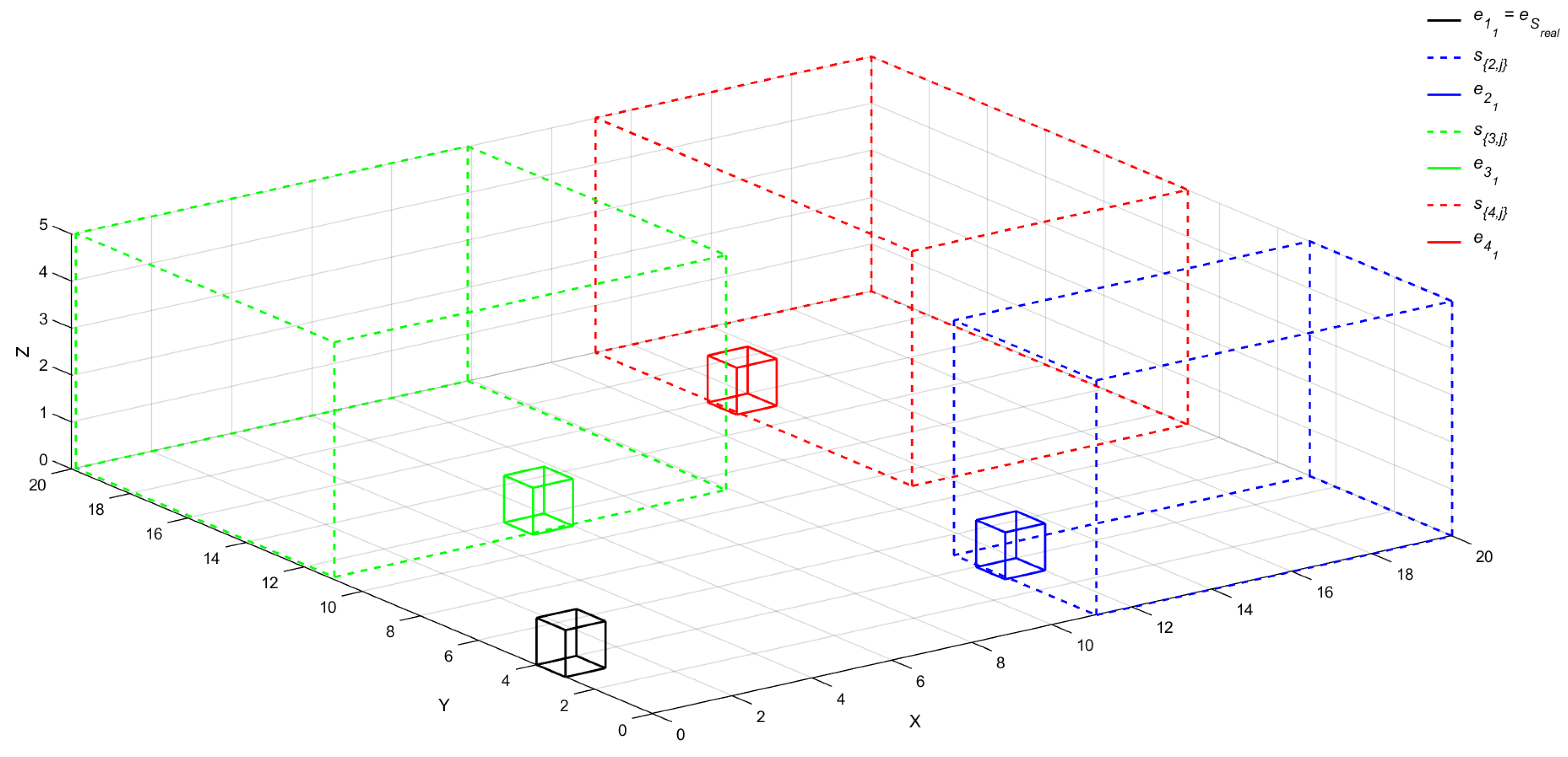
3.1. Space Representation

The presented algorithm uses a regular grid of cells as the exploration space $S_{real}$ (e.g., Figure 1 with four independent subspaces).

Definition 1.

Let $S_{real}=\{s_{\{1,2\}},s_{\{2,1\}},\dots ,s_{\{n,i\}}\}$ represent the space being explored, which consists of various subspaces $s_{\{n,i\}}$, where n represents the number of subspaces of the $S_{real}$ space and i represents the number of subspace types (e.g., land, water, and air).

Every subspace comprises a single type of environment and there is a finite number of the existing environments. The space may also be divided by obstacles, such as walls into subspaces with one or more entrances, that an agent can use to enter the subspace $s_{\{n,i\}}$.

Definition 2.

Let there be a set of entrances $E_j=\{e_{j_1},e_{j_2},\dots ,e_{j_m}\}$ to the subspace $s_{\{j,i\}}$, where m is the number of entrances of the $s_{\{j,i\}}$ subspace and $s_{\{j,i\}}\in S_{real}$, $j\in <1,n>$, $E_j\exists e_{j_m}\bigvee e_{j_m}\subseteq E_j\subset s_{\{j,i\}}$. The entrance $e_{j_m}$ is a position where the agent may enter the subspace $s_{\{j,i\}}$.

Definition 3.

Let $S_{real}$ have an entrance $e_{S_{real}}$, $e_{S_{real}}\subset s_{\{n,i\}}$ that an agent, who can operate in the i type of space, may use to enter in its subspace $s_{\{n,i\}}$.

3.2. Agent Representation

Definition 4.

Let $A=\{A_1,A_2,\dots ,A_f\}$ be a set of agents, where $A_f$ represents a set of agents with the same type/ability, which can operate in the i subspace type, $f\in <1,i>$.

Definition 5.

Let $A_f=\{a_{\{f,k,1\}},a_{\{f,k,2\}},\dots ,a_{\{f,k,v\}}\}$ be a set of agents that can operate in the f subspace type $f\in <1,i>$, where k represents a subspace identifier, in which the agents are operating $k\in <1,n>$ and v represent a number of available agents for the exploration of this type f of space.

We assume that $\forall i\exists A_f$ with minimal $v=1$ (a number of available agents). This is a necessary condition so that the entire space $S_{real}$ can be explored by agents.

Definition 6.

The $A{s}_x=\{a_{\{f,x,1\}},a_{\{f,x,2\}},\dots ,a_{\{f,x,o\}}\}$ is a set of agents operated in a subspace $s_{\{x,f\}}$, $x\in <1,n>$, $f\in <1,i>,o\in <1,\mathrm{\parallel }{A}_f\mathrm{\parallel }>$.

Definition 7.

Let $S_{real}$ have an entrance $e_{S_{real}}$, $e_{S_{real}}\subset s_{\{n,i\}}$ that an agent $a_{\{i,n,v\}}$ may use to enter its subspace $s_{\{n,i\}}$ and start to fulfill an exploration task.

Definition 8.

The $a_{\{f,k,v\}}$ agent is represented by the following variables,

$$\begin{array}{cc}\hfill a_{\{f,k,v\}}=\{& TR{a}_{\{f,k,v\}},TC{a}_{\{f,k,v\}},CC{a}_{\{f,k,v\}},t{a}_{\{f,k,v\}},TPe{a}_{\{f,k,v\}},\hfill \\ \hfill & TR{r}_{\{f,k,v\}},TC{r}_{\{f,k,v\}},CC{r}_{\{f,k,v\}},t{r}_{\{f,k,v\}},TPe{r}_{\{f,k,v\}}\},\hfill \end{array}$$

(1)

where

• $TR{a}_{\{f,k,v\}}\left(TR{r}_{\{f,k,v\}}\right)$, respectively, are the time periods used when adding (removing) an agent into (from) the group $A{s}_k$;
• $TC{a}_{\{f,k,v\}}\left(TC{r}_{\{f,k,v\}}\right)$, respectively, are the thresholds on the number of conflicts required to initiate a request for adding (removing) an agent to (from) the group $A{s}_k$, and the following conditions must be met $TC{a}_{\{f,k,v\}}\le TR{a}_{\{f,k,v\}}$ ($TR{r}_{\{f,k,v\}}\ge TC{r}_{\{f,k,v\}}$);
• $t{a}_{\{f,k,v\}}\left(t{r}_{\{f,k,v\}}\right\})$, respectively, are timers of exploration time used when adding (removing) the agents;
• $CC{a}_{\{f,k,v\}}\left(CC{r}_{\{f,k,v\}}\right)$, respectively, are the conflict counters used when adding (removing) an agent into (from) the group $A{s}_k$; and
• $TPe{a}_{\{f,k,v\}}\left(TPe{r}_{\{f,k,v\}}\right)$, respectively, represent the thresholds on the pheromone levels for adding (removing) the agent to (from) the group $A{s}_k$.

Definition 9.

Let the agent $a_{\{f,k,v\}}$ operating in the subspace $s_{\{k,f\}}$ be at the entrance $e_{y_m}$ belonging to the subspace $s_{\{y,u\}}$ only if $s_{\{k,f\}}$ and $s_{\{y,u\}}$ are adjacent subspaces $y\sim k\vee k,y\in <1,n>$ and the type of spaces $f\sim u,\vee f,u\in <1,i>$ (otherwise, the robot would not need transport). Let us assume that there is an agent $a_{\{u,y,l\}}$ capable of operating in the subspace $s_{\{y,u\}}$ and waiting at the entrance $e_{k_m}$ to be transported (an agent $a_{\{u,y,l\}}$ cannot in $s_{\{k,f\}}$ space), and the agent $a_{\{f,k,v\}}$ can transport the agent $a_{\{u,y,l\}}$ to the entrance $e_{y_m}$ through the subspace $s_{\{k,f\}}$.

3.3. Pheromone Marks for an Indirect Communication between the Agents

The agents do not use targeted communication from agent to agent. Variable numbers of agents are coordinated based on their interactions with the evaporating pheromone marks in the environment $S_{real}$. Each cell of the cellular space $S_{real}$ is capable of being marked by pheromone values. The pheromones gradually evaporate over time. Thereby, each cell(x,y,z) $\in S_{real}$ accumulates a time volatile pheromone value

$$S_{real}(x,y,z)=\left\{Pe{x}_n(x,y,z)\left(t\right)\right\},$$

(2)

where $Pe{x}_n(x,y,z)\left(t\right)$ is the pheromone trace value (which indicates when the cell was visited for the last time) in a given cell at (x, y, z) coordinates of the subspace $s_{\{n,i\}}$ at time t: a cell(x,y,z) $\in s_{\{n,i\}}\vee s_{\{n,i\}}\in S_{real}$.

The entrance $e_{j_m}$ is at a position where an agent may enter the subspace $s_{\{j,i\}}$, and $e_{j_m}\subseteq E_j\subset s_{\{j,i\}}$. The entrance cells of the space $S_{real}$ include the following two pheromone values,

$$\begin{array}{c}\hfill e_{\left\{j_m\right\}}=\{Pen{a}_{\{j,m,i\}}\left(t\right),Pen{r}_{\{j,m,i\}}\left(t\right)\}\end{array}$$

(3)

where $Pen{a}_{\{j,m,i\}}\left(t\right)$ ($Pen{r}_{\{j,m,i\}}\left(t\right)$) is the level of the pheromone requiring the addition (removal) of an agent into (from) the group operating in the $s_{\{j,i\}}$ subspace, respectively. The $Pen{a}_{\{j,m,i\}}\left(t\right)$ ($Pen{r}_{\{j,m,i\}}\left(t\right)$) value indicates that there are too few (many) robots in the given subspace to accomplish the exploration/monitoring task, respectively.

Each agent $a_{\{f,k,v\}}$ has an empty map of the environment $S_{a_{\{f,k,v\}}}$ (3D cellular grid) at the start. In each iteration (the time slot, in which an agent moves from one cell to another), the actual cell of the agent’s environment map $S_{a_{\{f,k,v\}}}(x,y,z)$ is updated based on the measured pheromone values of the actual cell $Pe{x}_n(x,y,z)$ of the exploration space $S_{real}(x,y,z)$. The agent uses the map $S_{a_{\{f,k,v\}}}$ for navigation and as a type of memory.

The agents produce three types of pheromones:

• The first type indicates that there are too few agents in the given subspace to accomplish the task (exploration and monitor).
• The second type indicates that there are too many agents.
• The third type indicates the exploration/monitoring ability.

The agent representation is supplemented by the following pheromone variables,

$$\begin{array}{cc}\hfill a_{\{f,k,v\}}=\{& Pma{x}_{\{f,k,v\}},P{a}_{\{f,k,v\}},P{r}_{\{f,k,v\}}\},\hfill \end{array}$$

(4)

where $Pma{x}_{\{f,k,v\}}$ is the value of a level of the pheromone mark that indicates the exploration/monitoring ability, and $P{a}_{\{f,k,v\}}$$\left(P{r}_{\{f,k,v\}}\right\})$ is the value of the pheromone required for adding (removal of) an agent to (from) the group $A{s}_k$, respectively. An agent’s pheromone mark values are constant during the agent’s life.

4. The Algorithms

All agents use the same algorithm that controls the behavior of the robot (agent). It defines three main types of behavior with the relevant priorities (space exploration or monitoring, population size control, and transportation). The agent’s main task is space exploration (secondary to the space monitoring task) and to keep the agent population at a suitable size for the environmental exploration. The transportation task has the highest priority: if the agent is capable of transporting another agent, it will transport it to the desired location. The initial design of the algorithm as shown in Figure 2 was presented at International Conference on Robotics in Alpe-Adria-Danube Region [40].

In the following sections, Section 4.1, Section 4.2 and Section 4.3, we describe, in more detail, the exploration, population management, and transportation rules, respectively, that control the behavior of the agents. Section 4.4 contains a more detailed description of the priority rules of the agents. Figure 2 shows the pseudo-state diagram of the agent’s entire decision making process with color marked states for individual agent behavior. The meaning of the individual states is as follows.

• 0—An agent is waiting for a request;
• 1—An agent is moving to the entrance of the target subspace;
• 2—An agents is exploring or monitoring a space;
• 3—An agent has a request to add or to remove an agent related to its own group;
• 4—An agent has a request to add an agent into a group different than its own or agent found an entrance to new unexplored subspace;
• 5—An agent is waiting to be transported;
• 6—An agent is transporting another agent;
• 7—An agent is being transported by another agent.

4.1. Space Exploration/Monitoring Roles

State 2 in Figure 2 represents the space exploration/monitoring role. The exploration space $S_{real}$ is divided into regular cubic cells. The agent can move into one of the neighboring cells (3D Moore or Neumann neighborhood) or stay where it is (in the case of a collision) in every iteration of the time t. The movements of the agents that perform the exploration or monitoring tasks, are controlled by the following rules. The rules were adapted from a 2D scenario, described in our previous research [35], to a 3D scenario:

• If the agent’s neighboring cells contain at least some non-zero pheromone values, the agent attempts to find the neighboring cell with the lowest pheromone value $min\left(Pe{x}_n(a,b,c)\left(t\right)\right)$, $a\in <x-1,x+1>$, $b\in <y-1,y+1>$, $c\in <z-1,z+1>\bigvee$ cell$(a,b,c)\in s_{\{n,i\}}$. If there are multiple cells with the same low level of pheromones, then the agent chooses one of these cells at random. The agent moves to the selected cell in the next iteration if it does not conflict with other agents.
• If the cells neighboring the agent have only zero pheromone values, then the agent chooses at random one of these cells and stores the direction $RD$ it has decided to move to. The agent then continues to move in the chosen direction $RD$, $RD\in <1,Z^{+}>$ in the next iterations until its neighboring cells contain only zero pheromone values and if it does not conflict with other agents.
• If two or more agents intend to move into the same cell$(x,y,z)$, a conflict occurs. In this situation, one of the agents is chosen randomly as a winner and it moves to the given cell in the next iteration. All the remaining agents participating in the conflict stay in their positions and wait for the next random tournament.

When an agent $a_{\{f,k,v\}}$ visits a cell(x,y,z)$\in s_{\{k,f\}}$, it leaves there a pheromone mark $Pma{x}_{\{f,k,v\}}$. This information is recorded into the internal map of the agent $S_{a_{\{f,k,v\}}}$ as well. Let us take a cell(x,y,z) $\in s_{\{k,v\}}$, then the value of the pheromone mark $Pe{x}_k(x,y,z)\left(t\right)$ in the cell(x,y,z) of the $S_{real}$ or internal agent map $S_{a_{\{f,k,v\}}}$ at the time t is calculated as

$$R(x,y,z)\left(t\right)=\left\{\begin{array}{cc}0\hfill & \mathrm{agent}\mathrm{is}\mathrm{not}\mathrm{in}\mathrm{the}\mathrm{cell}(x,y,z)\mathrm{in}\mathrm{the}\mathrm{time}t\hfill \\ 1\hfill & \mathrm{agent}\mathrm{is}\mathrm{in}\mathrm{the}\mathrm{cell}(x,y,z)\mathrm{in}\mathrm{the}\mathrm{time}t\hfill \end{array}\right.,$$

(5)

$$\begin{array}{c}\hfill Pe{x}_k(x,y,z)\left(t\right)=\left\{\begin{array}{c}Pma{x}_{\{f,k,v\}}\ast R(x,y,z)\left(t\right)\hfill \\ \mathrm{if}Pe{x}_k(x,y,z)(t-1)==0\hfill \\ Pma{x}_{\{f,k,v\}}\ast R(x,y,z)\left(t\right)+Pe{x}_k(x,y,z)(t-1)-1\hfill \\ \mathrm{if}Pe{x}_k(x,y,z)(t-1)>0\hfill \end{array}\right..\end{array}$$

(6)

The parameter $Pma{x}_{\{f,k,v\}}$ represents the initial level of the pheromone mark. It is calculated at the start of the algorithm and it depends on the size of the exploring space. We have established in previous experiments that $Pma{x}_{\{f,k,v\}}$ should be equal or greater than the number of the cells in the exploration space $s_{\{k,f\}}$ [38]. The equations above are valid for all the cells of the $S_{real}$ or $S_{a_{\{f,k,v\}}}$. The parameter $R(x,y,z)\left(t\right)$ represents an agent’s localization matrix in the space $S_{real}$.

4.2. Population Management Role

The size of the population of the agents influences the performance of the algorithm. It is very difficult to control the number of the individuals in a group without the use of the pheromone marks. The pheromone marks are dynamic in time and it is not possible to determine when a cell was visited for the last time based on the pheromone value. The published experimental results (see Figure 1 in [40]) confirmed our assumption that increasing the number of the agents in the space increased the number of the conflicts between the agents, and the average number of completed explorations decreased when the space became overpopulated. This was also observed in a space with obstacles [39]. Therefore, we developed rules for decentralized population control. Our proposed approach enables the interaction of agents of different types that operate in different environments. The agents operate in groups defined by the boundaries of the subspaces. The population size control algorithm performs two basic tasks (represented by state 3 in Figure 2):

• adding agents into the group and
• removing agents from the group.

Let there be a set of agents A that contains all types of agents needed to explore all types of environments $S_{real}=\{s_{\{1,2\}},s_{\{2,1\}},\dots ,s_{\{n,i\}}\}$. This set is located at the main entrance $e_{S_{real}}$ to the space $S_{real}$. The agents wait at the entrance $e_{S_{real}}$, $e_{S_{real}}=e_{x_m}\subset s_{\{x,k\}}$$x\in <1,n>,k\in <1,i>$ and check the pheromone marks $Pen{a}_{\{y,m,j\}}\left(t\right),y\in <1,n>,j\in <1,i>$ at the entrance $e_{S_{real}}$.

4.2.1. Adding Agents into the Group

Adding agents to the group ensures that there is a sufficient number of agents $a_{\{f,k,v\}}$ in the given subspace $s_{\{k,f\}}$ so that it is effectively explored. This addition is not subject to any centralized control. It is based on indirect space coverage estimation by observing the number of conflicts between agents. Each agent $a_{\{f,k,v\}}$ records the number of conflicts locally in a conflict counter $CC{a}_{\{f,k,v\}}$ and checks the number of conflicts periodically after a period $TR{a}_{\{f,k,v\}}$ has elapsed. If $CC{a}_{\{f,k,v\}}\le TC{a}_{\{f,k,v\}}$, where $TC{a}_{\{f,k,v\}}$ is an user adjustable parameter, the agent goes to the entrance $e_{k_m}$ it used to enter the subspace $s_{\{k,f\}}$ and leaves a request there (a pheromone mark $P{a}_{\{f,k,v\}}$) for adding an agent into its group $A_{s_k}$. Always after $t{a}_{\{f,k,v\}}==TR{a}_{\{f,k,v\}}$ has elapsed, the agent resets its $CC{a}_{\{f,k,v\}}$ and $t{a}_{\{f,k,v\}}$ counters to zero regardless of if an addition criterion is satisfied or not.

$$\mathrm{if} t{a}_{\{f,k,v\}}==TR{a}_{\{f,k,v\}}\Rightarrow CC{a}_{\{f,k,v\}}=0,t{a}_{\{f,k,v\}}=0.$$

The addition request that the agent places at the entrance $e_{k_m}$ is represented by a pheromone mark $Pen{a}_{\{k,m,f\}}$. The value of $Pen{a}_{\{k,m,f\}}$ decreases in time:

$$\begin{array}{c}\hfill Pen{a}_{\{k,m,f\}}\left(t\right)=\left\{\begin{array}{c}a\ast P{a}_{\{f,k,v\}}\mathrm{if}Pen{a}_{\{k,m,f\}}(t-1)==0\hfill \\ a\ast P{a}_{\{f,k,v\}}+Pen{a}_{\{k,m,f\}}(t-1)-1\mathrm{if}Pen{a}_{\{k,m,f\}}(t-1)>0\hfill \end{array}\right.,\end{array}$$

(7)

where a is a constant, that is, 1 if the agent placed the request at the entrance $e_{k_m}$ in time $\left(t\right)$ or 0 if the agent did not. If another agent places an addition request as well, the $Pen{a}_{\{k,m,f\}}\left(t\right)$ increases by $P{a}_{\{f,k,v\}}$ according to the formula above. New agents are added from the agent group $A_f$ automatically, if the following condition is satisfied,

$$Pen{a}_{\{k,m,f\}}\left(t\right)\ge TPe{a}_{\{f,k,v\}}\bigvee (e_{k_m}==e_{S_{real}})\subseteq s_{\{k,f\}}.$$

(8)

If $(e_{k_m}\ne e_{S_{real}})\bigvee (e_{y_m}==e_{S_{real}})\subseteq s_{\{y,l\}}\bigvee s_{\{y,l\}}$ and $s_{\{k,f\}}$ are adjacent subspecies, then agent $a_{\{l,y,v\}}$, operating in $s_{\{y,l\}}$, transfers the request from $e_{k_m}$ to $e_{y_m}$ (a more detailed explanation is in Section 4.3.3).

The following conditions must be also satisfied,

$$TC{a}_{\{f,k,v\}}\le TR{a}_{\{f,k,v\}}\le P{a}_{\{f,k,v\}}.$$

(9)

If $TR{a}_{\{f,k,v\}}\le P{a}_{\{f,k,v\}}$ is not satisfied, then no agent is added into the group $A_{s_k}$, because the pheromone $Pen{a}_{\{k,m,f\}}\left(t\right)$ at the entrance $e_{k_m}$ was reduced to 0 in a time that is greater than $TR{a}_{\{f,k,v\}}$. In other words, if the agents encounter each other too sporadically every agent that recognizes that the given subspace is sparsely populated (by counting conflicts over time) transfers a pheromone mark requesting adding an agent to the entrance. Several agents must do the same for the pheromone mark to become strong enough to exceed the threshold for adding an agent. If an agent comes to the entrance from the outer side of the underpopulated subspace and it encounters the pheromone mark placed at the entrance, it enters the subspace as a consequence.

4.2.2. Removing Agents from the Group

Removing agents from the group is a rule working against the addition rule. Therefore, it is important for these two behaviors to be in balance. An agent may fail temporarily in real-life situations. If the problem persists for long enough, the agent is replaced by another one that is added to the group. If the failure is resolved, for example, the agent’s battery is recharged from a solar panel, this re-enabled agent becomes redundant. The removal rule works to avoid congestion. If an agent $a_{\{f,k,v\}}$, while exploring the subspace $s_{\{k,f\}}$, records more conflicts than $TC{r}_{\{f,k,v\}}$ (i.e., $CC{r}_{\{f,k,v\}}\ge TC{r}_{\{f,k,v\}}$) or more conflicts than $TC{r}_{\{f,k,v\}}$ during the period $t{r}_{\{f,k,v\}}=TR{r}_{\{f,k,v\}}$, then the agent transfers a pheromone mark $P{r}_{\{f,k,v\}}$ to the entrance $e_{k_m}$ it has previously used to enter the subspace. The pheromone mark $Pen{r}_{\{k,m,f\}}\left(t\right)$ requests the removal of an agent from the group. The agent then resets its $CC{r}_{\{f,k,v\}}$ and $t{r}_{\{f,k,v\}}$ to zero even if $t{r}_{\{f,k,v\}}==TR{r}_{\{f,k,v\}}$ is not satisfied.

$$\mathrm{if} t{r}_{\{f,k,v\}}==TR{r}_{\{f,k,v\}}\Rightarrow CC{r}_{\{f,k,v\}}=0),t{r}_{\{f,k,v\}}=0.$$

The agent removal requesting the pheromone mark $Pen{r}_{\{k,m,f\}}\left(t\right)$ at the entrance $e_{k_m}$ decreases (evaporates) in time:

$$Pen{r}_{\{k,m,f\}}\left(t\right)=\left\{\begin{array}{c}b\ast P{r}_{\{f,k,v\}}\mathrm{if}Pen{r}_{\{k,m,f\}}(t-1)==0\hfill \\ b\ast P{r}_{\{f,k,v\}}+Pen{r}_{\{k,m,f\}}(t-1)-1\mathrm{if}Pen{r}_{\{k,m,f\}}(t-1)>0\hfill \end{array}\right.,$$

(10)

where b is equal to 1 if the agent placed the request at the entrance $e_{k_m}$; otherwise, 0. If another agent places a removal request too, $Pen{r}_{\{k,m,f\}}\left(t\right)$ increases by $P{r}_{\{f,k,v\}}$ according to the formula above. An agent may be removed from the group only if it is in the process of space exploration (state 2 in Figure 2). When an agent $a_{\{f,k,v\}}$ comes near the entrance $e_{k_m}$ and the pheromone mark $Pen{r}_{\{k,m,f\}}\left(t\right)$ is strong enough, it leaves the subspace through the entrance. This happens if

$$Pen{r}_{\{k,m,f\}}\left(t\right)\ge TPe{r}_{\{f,k,v\}}.$$

(11)

The condition that an agent may be removed from the group only if it is in state 2 eliminates the possibility of an agent to be removed by itself. Several agents must place the request in succession for the mark to become strong enough.

4.3. Transportation Role

We assume that every agent is capable of transporting (carrying) another agent through the environment in which the agent operates or requests (Definition 9). This is used when, for example, a watercraft discovers an island that it is not able to explore. The watercrafts may then transport land vehicles to the island. Transport of the agents and the management of the transportation requests consists of the following processes,

• the agent’s transportation (represented by states 5–7 in Figure 2),
• the creation of an addition request related to a different environment than the environment the given agent is capable of operating within (represented by state 4 in Figure 2), and
• the transfer of an addition request related to a group that is different than the group of the given agent (represented by state 4 in Figure 2).

4.3.1. Transport of an Agent

Let there be a set of agents A that contains all types of agents needed to explore all types of environments $S_{real}=\{s_{\{1,2\}},s_{\{2,1\}},\dots ,s_{\{n,i\}}\}$. This set is located at the main entrance $e_{S_{real}}$ to the space $S_{real}$. The agents wait at the entrance $e_{S_{real}}$, $e_{S_{real}}=e_{x_m}\subset s_{\{x,k\}}$$x\in <1,n>,k\in <1,i>$ and check the pheromone marks $Pen{a}_{\{y,m,j\}}\left(t\right),y\in <1,n>,j\in <1,i>$ at the entrance $e_{S_{real}}$. In the case that there is a pheromone mark placed at the entrance that informs of a needed addition of an agent from the agent group $A_j$ into the environment $s_{\{y,j\}}$, agent $a_{\{j,y,v\}}$ then accepts the request and goes to the given entrance $e_{S_{real}}$ (the pheromone mark $Pen{a}_{\{y,m,j\}}$ is then reset to zero).

If the agent $a_{\{j,y,v\}}$ is not capable of traversing the given type of environment $s_{\{x,k\}}$, $k\sim j\vee k$, $j\in <1,i>$ it waits then at the entrance and requests transport. If, during the process of space exploration, an agent $a_{\{k,x,v\}}$ comes to the vicinity of the agent $a_{\{j,y,v\}}$, then the agent $a_{\{k,x,v\}}$ automatically transports the agent $a_{\{j,y,v\}}$ to the entrance $e_{y_m}$ of the subspace $s_{\{y,j\}}$. Both agents resume the space exploration task upon the arrival at the target location. The pheromone mark encodes in itself the individual entrances it has been transported through.

4.3.2. Creating a Request for Adding an Agent into a Subspace with an Environment Where the Request Creating Agent is Not Capable of Operation

If the agent $a_{\{k,x,v\}}$ exploring a subspace $s_{\{x,k\}}$ finds the entrance $e_{y_m}\subset s_{\{y,j\}}$ to the subspace $s_{\{y,j\}}$, $x\sim y\vee x,y\in <1,n>$, and it is not capable of exploring the subspace $s_{\{y,j\}}$ (its abilities, construction, etc. prohibit it), and the entrance $e_{y_m}$ was not marked by the pheromone mark of the agent $a_{\{j,y,v\}}$, then the agent $a_{\{k,x,v\}}$ goes to the entrance $e_{x_m}\subset s_{\{x,k\}}$ it used to enter the subspace $s_{\{x,k\}}$ and leaves there a pheromone mark requesting the addition of a corresponding agent from the set $A_y$ ($Pen{a}_{\{y,m,j\}}$ from $e_{y_m}$ is transported to the $e_{S_{real}}$). If the entrance $e_{y_m}$ was already marked by the pheromone mark of the agent $a_{\{j,y,v\}}$, the agent $a_{\{k,x,v\}}$ continues to explore the subspace $s_{\{x,k\}}$.

4.3.3. Transfer of the Addition Request Related to the Addition of an Agent into a Group that Is Different than the Group of the Transferring Agent

Sometimes an agent that is needed elsewhere must transit several environments until it reaches the environment where it is capable of operating in. In that case, the problem of transferring the addition requests must be resolved. Let us assume that the subspace $S=\{s_{\{1,f\}},s_{\{2,d\}}\},f,d,\in <1,i>$ must be explored. Let $s_{\{1,f\}}$, $s_{\{2,d\}}$ have entrances $E_1=\left\{e_{1_z}\right\}$, $e_{S_{real}}=e_{1_z}\subset s_{\{1,f\}}$ and $E_2=\left\{e_{2_m}\right\},e_{2_m}\subset s_{\{2,d\}}$, respectively. Let us assume that $s_{\{2,d\}}$ is enveloped by $s_{\{1,f\}}$. There are agents $a_{\{f,1,v\}}$ operating in the subspace $s_{\{1,f\}}$ and $a_{\{d,2,x\}}$ operating in the subspace $s_{\{2,d\}}$ (the agent $a_{\{d,2,x\}}$ reached the subspace $s_{\{2,d\}}$, based on the previous two rules described in Section 4.1). If the agent $a_{\{d,2,x\}}$ operating in the subspace $s_{\{2,d\}}$ establishes that another agent is needed, agent $a_{\{d,2,x\}}$ goes to the entrance $e_{2_m}$ to the subspace $s_{\{2,d\}}$ to place the pheromone mark $P{a}_{\{d,2,x\}}$.

The value of the pheromone mark requesting the addition of an agent $Pen{a}_{\{2,m,d\}}\left(t\right)$ changes based on Equation (7) as the pheromone mark evaporates over time. If the agent $a_{\{f,1,v\}}$ operating in $s_{\{1,f\}}$ finds that the value of the pheromone mark requesting the addition of an agent $Pen{a}_{\{2,m,d\}}\left(t\right)$, at the entrance $e_{2_m}$, exceeds the threshold value $TPe{a}_{\{d,2,x\}}$, it takes the request; the value of $Pen{a}_{\{2,m,d\}}\left(t\right)$ is set to zero and transfers the request to the entrance it has previously used to enter the actual subspace $e_{1_z}$. As the entrance $e_{1_z}=e_{S_{real}}$ is checked by all types of agents, the appropriate agent takes the request and continues to explore the subspace or awaits being transported.

4.4. Priority Rules

The agents are capable of recognizing what state their neighboring agents (the “neighbors” in terms of Moore neighborhood cells $(a,b,c)\in s_{\{n,i\}},a\in <x-1,x+1>,b\in <y-1,y+1>$, $c\in <z-1,z+1>$) are in and what request they carry. Sometimes the agents decide to change their own state based on the state of the neighboring agents. This happens only if the agents are in state 2, 3, or 4 (see Figure 2) and the following rules apply.

-

If all the neighbors are in state 3 and carry the same request (either to add or to remove an agent) then one of them is chosen randomly to remain in state 3 and the remaining agents change their state from 3 to 2 and reset their parameters $CC{a}_{\{f,i,v\}}=0$, $t{a}_{\{f,i,v\}}=0$, $CC{r}_{\{f,i,v\}}=0$, $t{r}_{\{f,i,v\}}=0$; otherwise, (all the neighbors are in state 3 but carry different requests) all the neighbors change their state to 2 and reset their parameters to zero;

-

otherwise, if the neighbors are in states 2 and 3 then one of them is randomly chosen to remain in state 3 and the remaining agents change their state to 2; the agents in state 2 reset their counters $CC{a}_{\{f,i,v\}}=0$, $t{a}_{\{f,i,v\}}=0$, $CC{r}_{\{f,i,v\}}=0$, $t{r}_{\{f,i,v\}}=0$;

-

otherwise, if the neighbors are in state 4 but they must carry the same request and in state 2 one of them is chosen randomly to remain in state 4 and the remaining agents change their state to 2; the agents in state 2 reset their counters $CC{a}_{\{f,i,v\}}=0$, $t{a}_{\{f,i,v\}}=0$, $CC{r}_{\{f,i,v\}}=0$, $t{r}_{\{f,i,v\}}=0$;

-

otherwise, if the neighbors are in other states they will remain in their respective states and reset their counters.

Sometimes more robots with different requests intend to enter the same entrance. The agents then enter the entrance by priority. An agent in state 6 has the highest priority followed by states 3, 4, 7, 2, and 1 having the lowest priority. The above rules reduce the number of conflicts arising near the entrances and prevent oscillations in the population size.

5. Experiments

In order to evaluate the validity and performance of the algorithm, two experimental scenarios were established: The first scenario contained simple experiments with a single environment and with one type of agents with properties as defined in Chapter 4. The scenario containing experiments in a single environment with one agent type was designed to find the optimal parameters that influence the behavior of the swarm system of agents. In this scenario, there was a starting point $e_{S_{real}}$ in three-dimensional space $S_{real}$ from where the agents enter the environment. The $e_{S_{real}}$ and the entrances of the individual subspaces are also used for adding and removing the agents. The agents have a constant maximum speed of one cell per iteration and all agents are operated by the same high level strategic algorithm settings (the basic idea of a swarm), here we do not deal how different agent types are controlled at a lower level to achieve desired movement in a particular environment. The simple experiments were divided into three experiments:

• experiments focused on the dynamic addition of agents,
• experiments focused on the dynamic removal of agents, and
• experiments focused on the interaction between the dynamic removal and addition.

The second scenario contains a set of complex experiments with the exploration space consisting of multiple environments explored by multiple types of agents.

5.1. Simple Experiments—The Dynamic Addition of Agents

The main reason for executing this type of experiment was to investigate the influence of the parameters ($TPe{a}_{\{f,k,v\}}$, $TC{a}_{\{f,k,v\}}$, $TR{a}_{\{f,k,v\}}$, $P{a}_{\{f,k,v\}}$) on the behavior of the addition mechanism. The exploration space was sized 10 × 8 × 5 cells. Every value that is presented in the chart was calculated as the average value of five repetitions of the experiment. Every repetition had 10,000 iterations. The value of the pheromone $P{a}_{\{f,k,v\}}$ was set to $Pma{x}_{\{f,k,v\}}$ (therefore the parameter $TR{a}_{\{f,k,v\}}\le P{a}_{\{f,k,v\}}$ has to be set by this rule).

Figure 3 shows the number of agents added into the group in the 10,000th iteration based on two different initial pheromone mark settings. The parameter $TR{a}_{\{f,k,v\}}$, expressed as a percentage of $Pma{x}_{\{f,k,v\}}$, is on the X axis, and the Y axis shows the number of agents added into the group in the 10,000th iteration. Axis Z shows the value of $Pma{x}_{\{f,k,v\}}$. $TPe{a}_{\{f,k,v\}}$ is set to $TPe{a}_{\{f,k,v\}}=3\ast Pma{x}_{\{f,k,v\}}$ in Figure 3a, and $TPe{a}_{\{f,k,v\}}=5\ast Pma{x}_{\{f,k,v\}}$ in Figure 3b. Figure 4 shows another view of the results of the same experiments; however, the Y axis shows how many times the exploration space was explored (as the average from five repetitions of the experiments measured after 10,000 iterations). Different colors of the points represent the values of $TC{a}_{\{f,k,v\}}$.

The results demonstrated that, with the current parameter settings, adding more agents into the space led to a situation where the space was explored more times. We can also assume that decreasing $Pma{x}_{\{f,k,v\}}$ (resp. $P{a}_{\{f,k,v\}}$) leads to an increasing number of agents in the space. Decreasing $TR{a}_{\{f,k,v\}}$ had a similar effect. On the contrary, increasing $TC{a}_{\{f,k,v\}}$ increased the number of the agents in the space. The average number of conflicts between the agents increased with the number of the agents in the group. However, the graph is similar to the graph in Figure 4. The agents’ performance as a group is shown in the graph in Figure 5.

Our previous study of this algorithm proved that a group achieved the best results when $Pma{x}_{\{f,k,v\}}$ was roughly equal to the number of the cells of the explored space. This can be seen in Figure 5 ($Pma{x}_{\{f,k,v\}}=400\sim 450$, $TR{a}_{\{f,k,v\}}=90\%\sim 100\%$ of $Pma{x}_{\{f,k,v\}}$). A high value of $Pma{x}_{\{f,k,v\}}$ caused the agents to explore the entire space and then to decide whether or not they need help (therefore, we focus on this range of $Pma{x}_{\{f,k,v\}}$ in our investigation). The next part of Figure 5 shows the situation when $Pma{x}_{\{f,k,v\}}$ was set incorrectly with respect to $TR{a}_{\{f,k,v\}}$ (the number of explorations per agent in the group is less than three). Agents with this setting were unable to create a highly efficient group in the exploration space. Reducing $TR{a}_{\{f,k,v\}}$ led to a higher efficiency of the group. Figure 6 shows how the agents were added during the iterations. The curves represent (except for the graph in Figure 6) the averages of the population sizes measured in five experiments that lasted for 10,000 iterations.

5.2. Simple Experiments—The Dynamic Removal of Agents from the Group

We investigated the influence of $TR{r}_{\{f,k,v\}}$, $TC{r}_{\{f,k,v\}}$, $P{r}_{\{f,k,v\}}$, $Pen{r}_{\{j,m,i\}}$ (resp. $P{r}_{\{f,k,v\}}=Pma{x}_{\{f,k,v\}}$ on the removal of agents as shown in Figure 7). Again, the values in the graph represent averages acquired from five repetitions of the experiment. The sub-experiments were performed in an exploration space with the size of 10 × 8 × 5 cells, lasting for 30,000 iterations and starting with 50 agents exploring the space. The results indicated that lowering $TR{r}_{\{f,k,v\}}$ and $Pma{x}_{\{f,k,v\}}$ led to a larger population at the conclusion of the experiment. Figure 8 shows the result of the same experiment in the context of the number of explorations. The Y axis shows the number of space explorations after 30,000 iterations. There was a strong correlation between the results in Figure 7 and Figure 8.

The dynamics of the agent removal are shown in Figure 9 and Figure 10 (selected values only). The simulation results show that $Pen{r}_{\{k,m,f\}}$ determined the slope of the removal curve. $TC{r}_{\{f,k,v\}}$ and $TR{r}_{\{f,k,v\}}$ influenced the number of agents in the group after removal and the time needed to stabilize the group’s population (Figure 10). If $TC{r}_{\{f,k,v\}}$ and $TC{a}_{\{f,k,v\}}$ are set to similar values, the adaptation process will not stabilize (the agents will continue to be added and removed). If $TC{r}_{\{f,k,v\}}$ is large, many agents remain in the group during the removal process. This causes conflicts and negatively affects the number of explorations. $TR{r}_{\{f,k,v\}}$ must be set to interoperate with $TC{r}_{\{f,k,v\}}$. When $TC{r}_{\{f,k,v\}}$ is low and $TR{r}_{\{f,k,v\}}$ is high, the removal process may have a long duration because the agents meet scarcely (for example, in Figure 10 where $TR{r}_{\{f,k,v\}}=400\sim 500$). We also experimented with space sizes that were two and three times larger (Figure 11). The population size was again capable of adapting to the space size.

5.3. Simple Experiments—The Interaction between Dynamic Removal and Addition

These experiments investigated the whole process of the group size adaptation. The response of the system to the artificial addition and removal of the agents is illustrated in Figure 12 and Figure 13. We added 30 agents into the group in the 60,000th iteration and the group population was reduced to two agents in the 180,000th iteration in the experiment as shown in Figure 12. The group’s population stabilized with four agents during 5200 iterations. After the artificial addition of 30 agents into the group, the population stabilized at six agents during 5000 iterations.

This is ensured by the correct setting of $TR{r}_{\{f,k,v\}}$, $TC{r}_{\{f,k,v\}}$, and $Pen{r}_{\{j,m,i\}}$. The population in the group was reduced to two agents in the 180,000th iteration. The addition rules ensure that the population stabilizes before the artificial addition of agents. Figure 13 shows the result of an inappropriate setting of $Pma{x}_{\{f,k,v\}}$, $TR{a}_{\{f,k,v\}}$, and $TR{r}_{\{f,k,v\}}$. The population of the agents oscillates and this negatively affects the process of space exploration and monitoring.

We also investigated the group size adaptation to the size of the space (Figure 14). We added 30 agents into the group in the 6000th, 27,000th, and 56,000th iterations, and the group’s population was reduced to two agents in the 18,000th, 39,000th, and 67,000th iterations. Different curves in Figure 14 correspond to different space sizes. The results show that increasing the exploration space size leads to larger populations.

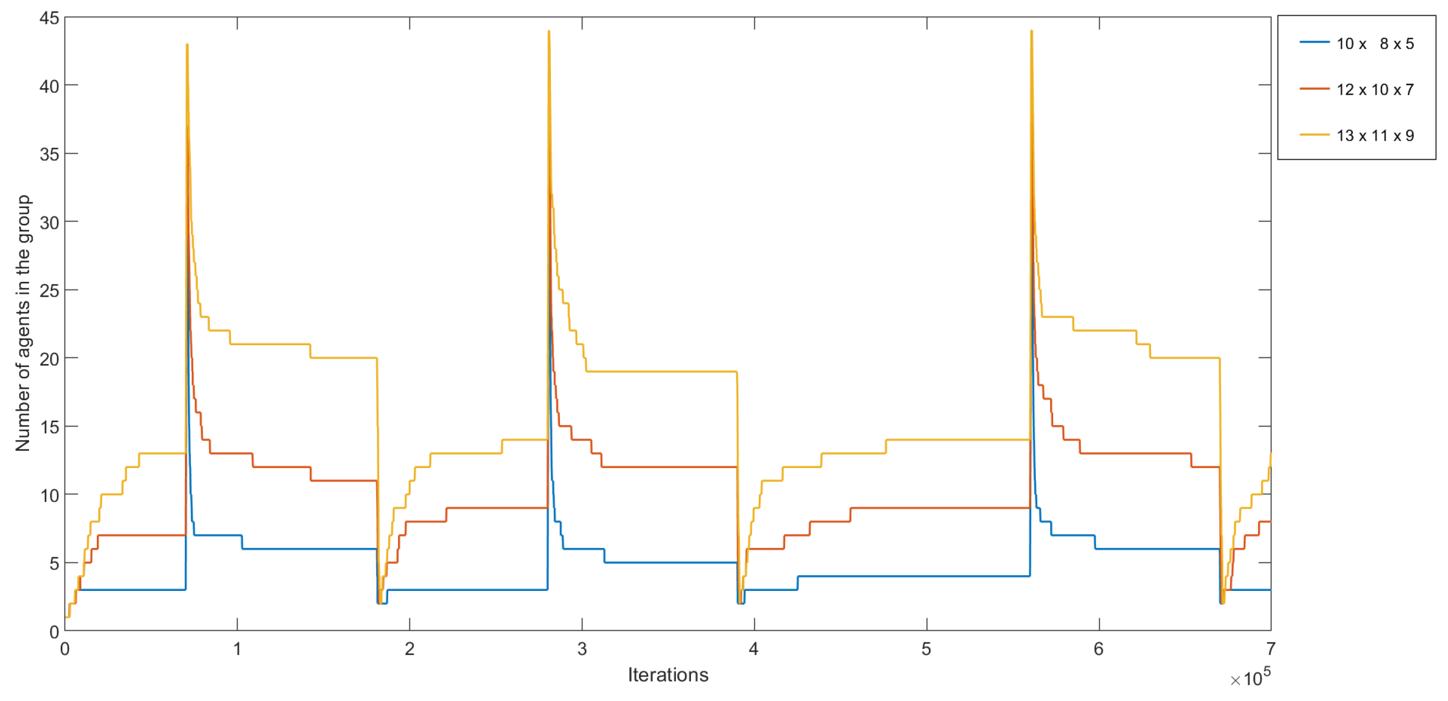
5.4. Complex Experiments—Experiments Focused on the Interactions between Dynamic Removal and Addition

The multi-environment exploration space $S_{real}$ contained two subspaces $S_{real}=\{s_{\{1,i\}},s_{\{2,j\}}\}$ in this experiment. The subspaces $s_{\{1,i\}}$ and $s_{\{2,j\}}$ have entrances $E_1=\left\{e_{1_1}\right\}$, $e_{1_1}\subseteq s_{\{1,i\}}$, and $E_2=\left\{e_{2_1}\right\}$, $e_{2_1}\subseteq s_{\{2,j\}}$, respectively. The subspaces are of equal size of 10 × 8 × 5 cells. The entrance $e_{1_1}$ is also the entrance to the space $S_{real}$, $e_{S_{real}}=e_{1_1}\subseteq s_{\{1,i\}}$. The subspace $s_{\{2,j\}}$ is enveloped by $s_{\{1,i\}}$. Agents are defined as general entities able to operate in a certain environment and transport other agents from one environment to another. The set of agents $A_i=\{a_{\{i,k,1\}},a_{\{i,k,2\}},\dots ,a_{\{i,k,25\}}\}$ can operate in the subspace $s_{\{1,i\}}$ and the set $A_j=\{a_{\{j,k,1\}},a_{\{j,k,2\}},\dots ,a_{\{j,k,25\}}\}$ in the subspace $s_{\{2,j\}}$. Each agent from the set $A_i$ can transport one agent from the set $A_j$ at a time from the $e_{S_{real}}$ to the $e_{2_1}$ of the subspace $s_{\{2,j\}}$ (Definition 9 and Section 4.3). The result of this experiment is shown in Figure 15. The subspaces were explored by groups of four agents.

Another experiment was focused on the investigation of the agents’ removal process following the artificial addition and removal of agents in heterogeneous space. The results are illustrated in Figure 16. The experiment was performed in a space that consisted of four subspaces $S_{real}=\{s_{\{1,i\}},s_{\{2,j\}},s_{\{3,j\}},s_{\{4,j\}}\}$ (the space illustrated in Figure 1). The subspaces had entrances $E_1=\left\{e_{1_1}\right\}$, $e_{1_1}\subseteq s_{\{1,i\}}$, $E_2=\left\{e_{2_1}\right\}$, $e_{2_1}\subseteq s_{\{2,j\}}$, $E_3=\left\{e_{3_1}\right\}$, $e_{3_1}\subseteq s_{\{3,j\}}$, and $E_4=\left\{e_{4_1}\right\}$, $e_{4_1}\subseteq s_{\{4,j\}}$. The sizes of the individual subspaces varied. The subspaces $s_{\{1,i\}}$, $s_{\{2,j\}}$, and $s_{\{3,j\}}$, and $s_{\{4,j\}}$ contained 865 cells, 250 cells, 500 cells, and 385 cells, respectively. The entrance $e_{1_1}$ was also the entrance to the space $S_{real}$, $e_{S_{real}}=e_{1_1}\subseteq s_{\{1,i\}}$. The subspaces $s_{\{2,j\}}$, $s_{\{3,j\}}$, $s_{\{4,j\}}$ were surrounded by $s_{\{1,i\}}$, but they were independent. The set of agents $A_i=\{a_{i,k,1},a_{i,k,2},\dots ,a_{i,k,25}\}$ contained agents that can operate in the subspace $s_{\{1,i\}}$. The set of agents $A_j=\{a_{\{j,k,1\}},a_{\{j,k,2\}},\dots ,a_{\{j,k,40\}}\}$ contains agents that can operate in the remaining subspaces $s_{\{2,j\}}$, $s_{\{3,j\}}$, and $s_{\{4,j\}}$.

The groups of agents explored the individual subspaces and successfully adapted their numbers to the sizes of the explored subspaces, it can thus be concluded that the algorithm is scalable. The $A_{s_2}$ ($A_{s_3}$, $A_{s_4}$) groups were operating in the subspaces $s_{\{2,j\}}$ ($s_{\{3,j\}}$, $s_{\{4,j\}}$), $A_{s_2},A_{s_3}$, and $A_{s_4}\in A_j\vee A_{s_2}\sim A_{s_3}\sim A_{s_4}$, respectively. Every agent of the $A_i$ set could transport one agent of the set $A_j$ at a time from $e_{S_{real}}$ to $e_{2_1}$, $e_{3_1}$, or $e_{4_1}$. Figure 17 illustrates the population growth in every subspace (each chart relates to one subspace). Small oscillations that are visible in the graphs occurred when agent $a_{\{i,1,x\}}$ transported an agent to another subspace. The oscillations in the other graphs occurred when agents from another subspaces brought agents to the current subspace.

6. Conclusions

We developed a novel complex algorithm that enabled the self-organization of a heterogeneous swarm of mobile agents, which operated in a set of different environments, and its functionality was proven as presented in the paper. The robots were reactive agents that communicated indirectly using simulated pheromone marks. We presented a short overview of the existing swarm approaches. We also described our previous work that led to the development of the novel algorithm that we presented here. All the realized experiments need to be taken as pilot experiments, which are aimed to prove that the whole concept is feasible and works. Completion of this goal has been demonstrated in two groups of goal oriented experiments.

First, we investigated the behavior of the agent robots controlled by our algorithm in a uniform environment populated with a swarm of agents robots of a single type. The experiments showed that our algorithm led to the stabilization of the population size in the swarm following the artificial addition or removal of some agents. In spite of the introduced disturbances, the results demonstrated that the population management was effective and did not affect the process of space exploration. Thus, we can attribute the property of robustness of the algorithm in case of acting disturbances; however, it needs to be noted that more experiments and theoretical work needs to be done to definitely prove it. This is one of the future aims of the research.

Then, we investigated the behavior of the algorithm in an exploration space containing multiple different environments. A transportation control algorithm that ensured the spreading of different types of agents across the exploration space with different types of environments was introduced and tested. This experiment shows that the designed concept is feasible and the mechanism for agents’ transportation works as designed and envisioned. We can consider this as a novel and unique feature of the algorithm that ensured that suitable robots were transported to the respective subspaces, in which they were capable of operating.

The experiments show that the algorithm has its inherent properties like scalability, failure tolerance, and the ability to explore all environments while transporting agents between them. This can be considered as a major and novel contribution in the field of agent swarm control algorithms. We found that our swarm control algorithm was able to successfully control three basic behaviors: space exploration, population management, and transportation. All these properties are combined in a single algorithm meaning that the behaviors were running simultaneously and space exploration (the main goal) was never stopped or interrupted. This is also an important feature of the algorithm and is shown in simulation experiments. The results demonstrated that, even if the space to be explored comprises different environments, the performance of the swarm was similar to the performance in a homogeneous environment, which is a great advantage of the algorithm. The algorithm was shown to be robust, fault tolerant, and independent of the environment where the agents worked. The swarm of agents adjusted its size autonomously accordingly to the size of the space to be explored and the optimal population size was reached in a finite time.

References

1. Margolus, N. Physics and Computation. Ph.D. Thesis, MIT Lab. for Computer Science, Cambridge, MA, USA, 1987. [Google Scholar]
2. Bijan, R.S.; Weiss, G.; Nakisaee, A. A Multi-Robot Coverage Approach Based on Stigmergic Communication. In German Conference on Multiagent System Technologies; Springer: Berlin/Heidelberg, Germany, 2012. [Google Scholar]
3. Ventocilla, E. Swarm-Based Area Exploration and Coverage based on Pheromones and Bird Flocks (Dissertation). 2013. Available online: http://urn.kb.se/resolve?urn=urn:nbn:se:uu:diva-212190 (accessed on 20 May 2020).
4. Iocchi, L.; Nardi, D.; Salerno, M. Reactivity and Deliberation: A Survey on Multi-Robot Systems. In Balancing Reactivity and Social Deliberation in Multi-Agent Systems; From RoboCup to Real-World Applications; Springer: Berlin, Germany, 2013; pp. 9–32. [Google Scholar]
5. Navarro, I.; Matía, F. An Introduction to Swarm Robotics. ISRN Robot. 2013, 2013, 1–10. [Google Scholar] [CrossRef] [Green Version]
6. Sahin, E. Swarm Robotics: From Sources of Inspiration to Domains of Application. In Swarm Robotics Workshop: State-of-the-Art Survey; Şahin, E., Spears, W., Eds.; Lecture Notes in Computer Science; Springer: Berlin, Germany, 2005; pp. 10–20. [Google Scholar]
7. Patil, M.; Abukhalil, T.; Patel, S.; Sobh, T. Ub swarm: Hardware implementation of heterogeneous swarm robot with fault detection and power management. Int. J. Comput. 2016, 15, 162–176. [Google Scholar]
8. Agmon, N.; Hazon, N.; Kaminka, G.A. The giving tree: Constructing trees for efficient offline and online multi-robot coverage. Ann. Math. Artif. Intell. 2008, 52, 143–168. [Google Scholar] [CrossRef]
9. Sauter, A.J.; Matthews, R.; Van, H.; Parunak, D.; Brueckner, A.B. Performance of Digital Pheromones for Swarming Vehicle Control. In Proceedings of Fourth International Joint Conference on Autonomous Agents and Multi-Agent Systems; ACM Press: Utrecht, The Netherlands, 2005; pp. 903–910. ISBN 1-59593-093-0. [Google Scholar] [CrossRef]
10. Senthilkumar, K.S.; Bharadwaj, K.K. Multi-robot exploration and terrain coverage in an unknown environment. Robot. Auton. Syst. 2012, 60, 123–132. [Google Scholar] [CrossRef]
11. Cheng, P.; Keller, J.; Kumar, V. Time-Optimal UAV Trajectory Planning for 3d Urban Structure Coverage. In Proceedings of the Intelligent Robots and Systems, IROS’08, Nice, France, 22–26 September 2008; pp. 2750–2757. [Google Scholar]
12. Hert, S.; Tiwari, S.; Lumelsky, V. A terrain-covering algorithm for an UAV. Auton. Robot. 2006, 3, 91–119. [Google Scholar] [CrossRef]
13. Lee, T.-S.; Choi, J.-S.; Lee, J.-H.; Lee, B.-H. 3-d Terrain Covering and Map Building Algorithm for an UAV. In Proceedings of the Intelligent Robots and Systems, IROS’09, St. Louis, MO, USA, 10–15 October 2009; pp. 4420–4425. [Google Scholar]
14. Atkar, P.N.; Choset, H.; Rizzi, A.A.; Acar, E.U. Exact Cellular Decomposition of Closed Orientable Surfaces Embedded in 3. In Proceedings of the 2001 ICRA IEEE International Conference on Robotics and Automation, Seoul, Korea, 21–26 May 2001; Volume 1, pp. 699–704. [Google Scholar]
15. Atkar, P.; Greenfield, A.L.; Conner, D.C.; Choset, H.; Rizzi, A. Uniform coverage of automotive surface patches. Int. J. Robot. Res. 2005, 24, 883–898. [Google Scholar] [CrossRef]
16. Oksanen, T.; Visala, A. Coverage path planning algorithms for agricultural field machines. J. Field Robot. 2009, 26, 558–651. [Google Scholar] [CrossRef]
17. Xu, A.; Viriyasuthee, C.; Rekleitis, I. Optimal Complete Terrain Coverage Using an Unmanned Aerial Vehicle. In Proceedings of the Robotics and Automation (ICRA), Shanghai, China, 9–13 May 2011; pp. 2513–2519. [Google Scholar]
18. Barrientos, A.; Colorado, J.; Cerro, J.; Martinez, A.; Rossi, C.; Sanz, D.; Valente, J. Aerial remote sensing in agriculture: A practical approach to area coverage and path planning for fleets of mini aerial robots. J. Field Robot. 2011, 28, 667–689. [Google Scholar] [CrossRef] [Green Version]
19. Kappel, K.S.; Cabreira, T.M.; Marins, J.L.; De Brisolara, L.B.; Ferreira, P.R. Strategies for Patrolling Missions with Multiple UAVs. J. Intell. Robot. Syst. 2019, 1–17. [Google Scholar] [CrossRef]
20. Abukhalil, T.; Patil, M.; Patel, S.; Sobh, T. Deployment environment for a swarm of heterogeneous robots. Robotics 2016, 5, 22. [Google Scholar] [CrossRef] [Green Version]
21. Cristobal, M.J. Autonomous Exploration and Mapping of Unknown Environments with Teams of Mobile Robots. 2013. Available online: http://docplayer.net/11615759-Autonomous-exploration-and-mapping-of-unknown-environments-with-teams-of-mobile-robots.html (accessed on 20 May 2020).
22. Ducatelle, F.; Di Caro, G.A.; Gambardella, L.M. Cooperative Self-Organization in a Heterogeneous Swarm Robotic System. In Proceedings of the 12th Annual Conference on Genetic and Evolutionary Computation (GECCO ’10), Portland, OR, USA, 7–11 July 2010; Association for Computing Machinery: New York, NY, USA, 2010; pp. 87–94. [Google Scholar] [CrossRef]
23. Zelinsky, A.; Jarvis, R.A.; Byrne, J.C.; Yuta, S. Planning Paths of Complete Coverage of an Unstructured Environment by a Mobile Robot. In Proceedings of International Conference on Advanced Robotics, Tsukuba, Japan, 8–9 November 1993; pp. 533–538. [Google Scholar]
24. Carsten, J.; Ferguson, D.; Stentz, A. 3D Field D: Improved Path Planning and Replanning in Three Dimensions. In Proceedings of the 2006 IEEE/RSJ International Conference on Intelligent Robots and Systems, IROS’06, Beijing, China, 9–15 October 2006; pp. 3381–3386. [Google Scholar]
25. Koenig, S.; Szymanski, B.; Liu, Y. Efficient and inefficient ant coverage methods. Ann. Math. Artif. Intell. 2011, 31, 41–76. [Google Scholar] [CrossRef]
26. Masár, M.; Budinská, I. Robot Coordination Based on Biologically Inspired Methods. In Advanced Materials Research; Trans Tech Publications Ltd.: Stafa-Zurich, Switzerland, 2013; Volume 664, pp. 891–896. [Google Scholar]
27. Burgard, W.; Moors, M.; Stachniss, C.; Schneider, F.E. Coordinated multi-robot exploration. IEEE Trans. Robot. 2017, 21, 376–386. [Google Scholar] [CrossRef] [Green Version]
28. Wagner, I.; Lindenbaum, M.; Bruckstein, A. Distributed Covering by Ant-Robots Using Evaporating Traces. IEEE Trans. Robot. Autom. 1999, 15, 918–933. [Google Scholar] [CrossRef] [Green Version]
29. Chu, H.; Glad, A.; Simonin o Sempe, F.; Drogoul, A.; Charpillet, F. Swarm Approaches for the Patrolling Problem, Information Propagationvs, Pheromone Evaporation. In Proceedings of the ICTAI’07 IEEE International Conference on Tools with Artificial Intelligence, Patras, Greece, 29–31 October 2007; pp. 442–449. [Google Scholar]
30. Yanovski, V.; Wagner, I.A.; Bruckstein, A.M. A Distributed Ant Algorithm for Efficiently Patrolling a Network. Algorithmica 2013, 73, 165–186. [Google Scholar] [CrossRef]
31. Rosalie, M.; Danoy, G.; Chaumette, S.; Bouvry, P. From Random Process to Chaotic Behavior in Swarms of UAVs. In Proceedings of the 6th ACM Symposium on Development and Analysis of Intelligent Vehicular Networks and Applications, Malta, Malta, 13–17 November 2016; pp. 9–15. [Google Scholar] [CrossRef] [Green Version]
32. Kilin, A.; Božek, P.; Karavaev, Y.; Klekovkin, A.; Shestakov, V. Experimental investigations of a highly maneuverable mobile omniwheel robot. Int. J. Adv. Robot. Syst. 2017, 14. [Google Scholar] [CrossRef]
33. Božek, P.; Blišťan, P.; Al Akkad, M.A.; Ibrahim, N.I. Navigation control and stability investigation of a mobile robot based on a hexacopter eqipped with an integrated manipulator. Int. J. Adv. Robot. Syst. 2017, 14. [Google Scholar] [CrossRef] [Green Version]
34. Patil, M.; Abukhalil, T.; Sobh, T. Hardware Architecture Review of Swarm Robotics System: Self-Reconfigurability, Self-Reassembly, and Self-Replication. ISRN Robot. 2013, 2013, 849606. [Google Scholar] [CrossRef]
35. Zelenka Jand Kasanický, T. Insect Pheromone Strategy for the Robots Coordination—Reaction on Loss Communication. In Proceedings of the 2014 IEEE 15th International Symposium on Computational Intelligence and Informatics (CINTI) 2014, Budapest, Hungary, 19–21 November 2014; pp. 79–83. [Google Scholar]
36. Zelenka, J.; Kasanický, T. Outdoor UAV Control and Coordination System Supported by Biological Inspired Method. In Proceedings of the 2014 23rd International Conference on Robotics in Alpe-Adria-Danube Region (RAAD) 2014, Smolenice, Slovakia, 3–5 September 2014; Slovak University of Technology in Bratislava: Bratislava, Slovakia, 2014. ISBN 978-1-4799-6798-8. [Google Scholar]
37. Cao, Y.U.; Fukunaga, A.S.; Kahng, A.B. Cooperative mobile robotics: Antecedents and directions. Auton. Robot. 1997, 4, 226–234. [Google Scholar] [CrossRef]
38. Zelenka, J.; Kasanický, T. Control and Coordination System Supported by Biologically Inspired Method for 3D Space “Proof of Concept”. In Advances in Intelligent Systems and Computing: Advances in Robot Design and Intelligent Control; Springer: Cham, Switzerland, 2015; Volume 371, pp. 147–156. ISBN 978-3-319-21289-0. [Google Scholar]
39. Zelenka, J.; Kasanický, T. Control and Coordination System Supported by Biologically Inspired Method for 3D Space “Performance improvements”. In Proceedings of the 2015 IEEE 19th International Conference on Intelligent Engineering Systems (INES), Bratislava, Slovakia, 3–5 September 2015; pp. 265–269, ISBN 978-1-4673-7938-0. [Google Scholar]
40. Zelenka, J.; Kasanický, T. A Self-adapting Method for 3D Environment Exploration Inspired by Swarm Behaviour. In Advances in Service and Industrial Robotics. RAAD 2017. Mechanisms and Machine Science; Ferraresi, C., Quaglia, G., Eds.; Springer: Cham, Switzerland, 2018; Volume 49. [Google Scholar]
Figure 1. A heterogeneous exploration space S r e a l consisting of three independent subspaces.
Applsci 10 03562 g001
Figure 2. Pseudo-state diagram of the agent’s entire decision making process (green represents population management behavior, purple represents exploration/monitoring behavior, and orange represents transportation behavior).
Applsci 10 03562 g002
Figure 3. The number of agents added in the group at the 10,000th iteration of the exploration process: P a { f , k , v } = P m a x { f , k , v } , the exploration space size represented 10 × 8 × 5 cells, T P e a { f , k , v } = 3 P m a x { f , k , v } , and T P e a { f , k , v } = 5 P m a x { f , k , v } .
Applsci 10 03562 g003
Figure 4. The number of explorations of the entire space in the 10,000th iteration: T P e a { f , k , v } = 3 P m a x { f , k , v } .
Applsci 10 03562 g004
Figure 5. The average number of explorations per agent at the 10,000th iteration: T P e a { f , k , v } = 3 P m a x { f , k , v } , P a { f , k , v } = P m a x { f , k , v } , and the exploration space was 10 × 8 × 5 cells.
Applsci 10 03562 g005
Figure 6. Adding the agents to the group for various parameter settings: T C a { f , k , v } = 0 , T R a { f , k , v } = 70 % from P m a x { f , k , v } , and T P e a { f , k , v } = 3 P m a x { f , k , v } .
Applsci 10 03562 g006
Figure 7. The number of the agents in the group after 30,000 iterations; we added 50 agents to the group in the 1000th iteration and removing agents was then turned off.
Applsci 10 03562 g007
Figure 8. The number of space explorations after 30,000 iterations; we added 50 agents to the group in the 1000th iteration and removing agents was then turned off.
Applsci 10 03562 g008
Figure 9. Removing agents from the group with dependence on T C r { f , k , v } and P e n r { j , m , i } ; the simulation lasted for 30,000 iterations; 50 agents were added into the group in the 1000th iteration: P m a x { f , k , v } = 400 , T R r { f , k , v } = 200 (a), and T R r { f , k , v } = 400 (b).
Applsci 10 03562 g009
Figure 10. Removing agents from the group with dependence on T R r { f , k , v } ; the simulation lasted for 30,000 iterations; 50 agents were added into the group in the 1000th iteration: P m a x { f , k , v } = 400 , T C r { f , k , v } = 8 and P e n r { j , m , i } = 5 P m a x { f , k , v } .
Applsci 10 03562 g010
Figure 11. The number of agents in the group with dependence on P m a x { f , k , v } ; experimenting with a removing agents in various space sizes; 50 agents were added into the group in the 1000th iteration: T C r { f , k , v } = 8 , T R r { f , k , v } = 200 , and P e n r { j , m , i } = 3 P m a x { f , k , v } .
Applsci 10 03562 g011
Figure 12. Adaptation of the group’s population in a space of 10 × 8 × 5 cells, simulated for 25,000 iterations: P m a x { f , k , v } = P a { f , k , v } = P r { f , k , v } = 400 , T C a { f , k , v } = 0 , T R a { f , k , v } = 280 , T C r { f , k , v } = 8 , T R r { f , k , v } = 100 , and P e n a { j , m , i } ( t ) = P e n r { j , m , i } = 3 P m a x { f , k , v } .
Applsci 10 03562 g012
Figure 13. Adaptation of the group’s population in a space of 10 × 8 × 5 cells, simulated for 25,000 iterations, P m a x { f , k , v } = P a { f , k , v } = P r { f , k , v } = 200 , T C a { f , k , v } = 0 , T R a { f , k , v } = 100 , T C r { f , k , v } = 8 , T R r { f , k , v } = 200 and P e n a { j , m , i } ( t ) = P e n r { j , m , i } = 3 P m a x { f , k , v } .
Applsci 10 03562 g013
Figure 14. Adaptation of the group’s population in spaces of various sizes, simulated for 700,000 iterations: P m a x { f , k , v } = P a { f , k , v } = P r { f , k , v } = 400 , T C a { f , k , v } = 0 , T R a { f , k , v } = 280 , T C r { f , k , v } = 8 , T R r { f , k , v } = 100 , and P e n a { j , m , i } ( t ) = P e n r { j , m , i } = 3 P m a x { f , k , v } , space sizes 10 × 8 × 5, 12 × 10 × 7 and 13 × 11 × 9 cells. We added 30 agents into the group in the 6000th, 27,000th, and 56,000th iteration and the group’s population was reduced to two agents in the 18,000th, 39,000th, and 67,000th iterations.
Applsci 10 03562 g014
Figure 15. The exploration of heterogeneous space, simulated for 30,000 iterations: P m a x { f , k , v } = P a { f , k , v } = P r { f , k , v } = 400 , T C a { f , k , v } = 0 , T R a d d v = 280 , T C r { f , k , v } = 8 , T R r { f , k , v } = 100 , and P e n a { j , m , i } ( t ) = P e n r { j , m , i } = 3 P m a x { f , k , v } .
Applsci 10 03562 g015
Figure 16. The exploration of heterogeneous space with the artificial addition and removal of the agents to and from A 1 and A 2 groups: P m a x { f , k , v } = P a { f , k , v } = P r { f , k , v } = 400 , T C a { f , k , v } = 0 , T R a { f , k , v } = 280 , T C r { f , k , v } = 8 , T R r { f , k , v } = 100 , and P e n a { j , m , i } ( t ) = P e n r { j , m , i } = 3 P m a x { f , k , v } .
Applsci 10 03562 g016
Figure 17. The number of agents in the groups operating in the individual subspaces of the multi-environment space (Figure 1).
Applsci 10 03562 g017