Ensemble Model Based on Stacked Long Short-Term Memory Model for Cycle Life Prediction of Lithium–Ion Batteries


Department of Industrial Management, National Taiwan University of Science and Technology, Taipei 10607, Taiwan
*
Author to whom correspondence should be addressed.
Appl. Sci. 2020, 10(10), 3549; https://doi.org/10.3390/app10103549
Submission received: 24 March 2020
/
Revised: 15 May 2020
/
Accepted: 19 May 2020
/
Published: 20 May 2020
(This article belongs to the Special Issue Chemistry for Lithium Metal Batteries)
Abstract
:To meet the target value of cycle life, it is necessary to accurately assess the lithium–ion capacity degradation in the battery management system. We present an ensemble model based on the stacked long short-term memory (SLSTM), which is used to predict the capacity cycle life of lithium–ion batteries. The ensemble model combines LSTM with attention and gradient boosted regression (GBR) models to improve prediction accuracy, where these individual prediction values are used as input to the SLSTM model. Among 13 cells, single and multiple cells were used as the training set to verify the performance of the proposed model. In seven single-cell experiments, 70% of the data were used for model training, and the rest of the data were used for model validation. In the second experiment, one cell or two cells were used for model training, and other cells were used as test data. The results show that the proposed method is superior to individual and traditional integrated learning models. We used Monte Carlo dropout techniques to estimate variance and obtain prediction intervals. In the second experiment, the average absolute percentage errors for GBR, LSTM with attention, and the proposed model are 28.6580, 1.7813, and 1.5789, respectively.
1. Introduction
Lithium–ion (Li–ion) batteries have the advantages of low cost, high energy density, and long service life so that they can be widely used in mobile electronics and automotive industries [1,2]. For all battery chemistries, Li–ion batteries degrade with each charge and discharge cycle. Therefore, the accurate description and estimation of the degradation process of lithium–ion batteries have become an important issue, in which the battery health status (SOH) and remaining useful life (RUL) are two important indicators [3,4]. The accurate estimated value of SOH can make users maintain the battery more reasonably, to improve the safe usage rate of the battery [5,6]. SOH is the indicator of the present performance of the battery in terms of either capacity or resistance/power, while RUL indicates the rest of the combined cycle and calendar life until the predefined end-of-life (EOL) level is achieved.
Model methods, data-driven methods, and hybrid methods often perform capacity reduction and cycle life prediction. Model-based methods are based on degraded empirical or physical models; however, constructing such a mathematical model is not an easy task. This method does not require large amounts of data. The data-driven approach can capture strong nonlinearities without prior system knowledge. Data-driven methods have been commonly used to predict cycle life and can represent the inherent relationship of the battery without requiring professional knowledge of degradation mechanisms [7]; however, this method requires a lot of data and computational cost. Hybrid methods show great potential for better prediction accuracy than model-based and data-driven prediction methods [8]. Ensemble learning technology is one of the most popular hybrid methods, which improves prediction accuracy by combining multiple learning algorithms [9]. The ensemble learning method is a learning algorithm that can aggregate predictions generated by multiple learning algorithms to enhance prediction performance.
Previous research has shown that ensemble learning algorithms generally outperform any individual learning algorithm [9,10,11,12,13]. Most ensemble methods use the average value of multiple models as the final prediction result; however, the prediction of ensemble learning in regression problems does not necessarily guarantee that its prediction results will be better than a single model. Therefore, a new method needs to be developed to test whether an ensemble model combining multiple learning algorithms can provide better prediction performance than a single model. The long short-term memory (LSTM) recurrent neural network (RNN) was used to analyze the capacity degradation of lithium–ion batteries [14]. The LSTM model can be extended and added to other mechanisms such as bidirectional, stacked, and attention mechanisms.
In this study, we propose an ensemble model based on a stacked long short-term memory (SLSTM) model to the cycle life estimation of lithium–ion batteries. The final prediction output was obtained by stacking LSTM models, rather than taking the average of the prediction values of each model. Besides, the selected features and optimal hyperparameter values may affect the accuracy of cycle life prediction. Few studies consider multiple features as input to the model. For example, Chen et al. [15] and Wang and Mamo [16] used support vector machines with multiple features such as cycle and temperature to predict the SOH of lithium–ion batteries. The best model hyperparameters are obtained by using the differential evolution (DE) algorithm, and several features were also considered in this study. LSTM with attention and gradient boosted regression (GBR) models were used as two single models. Section 2 and Section 3 describe the experimental data and a detailed description of the proposed model, respectively. Section 4 describes model verification. Finally, we summarize the conclusions and future research directions.
2. Experimental Data
Thirteen cells from commercial Lithium Ferrous Phosphate (LFP)/graphite (A123 Systems, model APR18650M1A, 1.1 Ah rated capacity) [2] were used for model verification. These 13 cells were cycled in a temperature-controlled environmental chamber (30 °C) under various fast charging policies and discharged with a constant-current constant-voltage (CC-CV) discharge at 4 C to 2.0 V with a current cutoff of C/50. The rated capacity of each unit is 1.1 Ah, and the rated voltage is 3.3 V.
The entire data set consisted of three batches of cells running in parallel. The cell was tested using a two-step fast charging policy. For example, a two-step strategy might include a 6 C charging step from 0% to 50% state-of-charge (SOC), followed by a 4 C charging step from 50% to 80% SOC. The 72 charging policies represent different combinations of current steps in the 0% to 80% SOC range [2]. The batch test conditions were slightly different. For the “2017-05-12” batch, after reaching 80% SOC, the test conditions during charging and after discharging were 1 min and 1 s, respectively. For the “2017-06-30” batch, after reaching 80% SOC, the test conditions during charging and after discharging were both 5 min. For the “2018-04-12” batch, after reaching 80% SOC, the test time during the charging process, after the internal resistance test and before and after discharging, was 5 s.
For model verification, we selected thirteen cells from the “2017-05-12” and “2017-06-30” batches. Table 1 shows the representation of 13 cells with their charging policies. In the first experiment, seven cells are used, where the first 70% of the data on each cell was used for model training to predict the remaining discharge capacity. In the second experiment, two groups (cell 1, cell 2, and cell 3) and (cell 2_25, cell 2_26, and cell 2_27) were used, where the test condition of each group is under the same charging policy. Several features such as discharge capacity, cycle number, temperature, and internal resistance for each cell were used for model training to evaluate the performance of the proposed model.
3. Prediction Models
In this study, we propose an ensemble model based on the SLSTM model for cycle life prediction. The ensemble model is based on two models, LSTM with attention and GBR models, which are introduced in this subsection.
3.1. LSTM with an Attention Mechanism
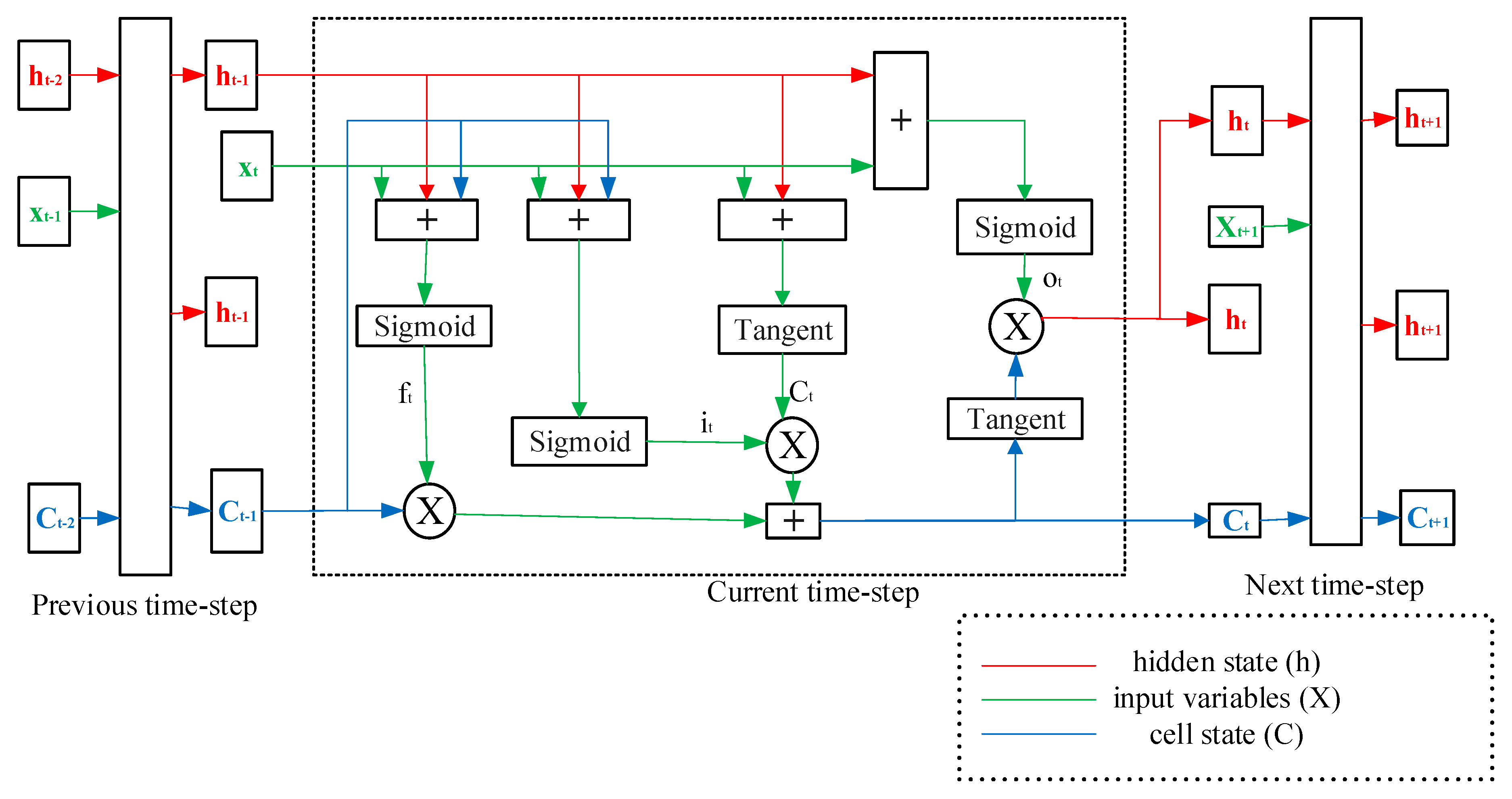
Although the standard recurrent neural network is an extension of the conventional feed-forward neural network, it has the problem of gradient vanishing or explosion. LSTM was developed to solve these problems and achieve excellent performance. It has unique memory and forgetting modes and can be flexibly adapted to the timing characteristics of network learning tasks. The units of the LSTM model includes a forget gate, input gate, and output gate [17,18]. The forget gate is designed to determine whether it needs to be discarded from the cell state. The input gate is designed to determine whether new information should be stored in the cell state. The output gate is designed to determine what information will be transferred from the cell state to the current hidden layer data. These gating units are derived by
where is the sigmoid function to keep the output value between 0 and 1; ht−1 and Xt are previous layer data and the current input layer data; are the input weight, the recurrent weight, and the bias of a forget gate.
where are the input weight, the recurrent weight, and the bias of an input gate. A tanh layer is chosen to form the new memory as where are the input weight, the recurrent weight, and the bias of a new memory. Then, the cell state is updated by .
where are the input weight, the recurrent weight, and the bias of an output gate. Finally, we multiply it by the output of the sigmoid gate as . Figure 1 shows the architecture of the LSTM cell.
Recently, the attention mechanism is usually used to analyze images and time-series data. Compared with other ordinary deep learning models, combining attention with LSTM can obtain better results. Note that the attention layer only helps to select the output of earlier layers that are critical to each subsequent stage of the model. It allows the network to focus on specific information selectively. It is accomplished by building a neural network focused on appropriate tasks. Detailed information on the attention-based LSTM model can be found in [21,22,23,24]. In this study, the attention-based LSTM model is used as a single model. The best model parameters are obtained from the DE algorithm.
3.2. Gradient Boosted Regression
Gradient boosting is a useful machine learning model that can obtain accurate results in various practical tasks. It focuses on the errors caused by each step iteratively until the weak learners are combined by finding suitable strong learners as the sum of consecutive weak learners [25,26,27]. The boosting iteration can be based on functional gradient descent. Let S = be samples. A function is used to predict values based on the local loss function . We minimize the expected value of the loss function to obtain the approximate value of the function f(x). GBR follows the regularization-method based on shrinkage and updates in each corresponding area as follows:
where is called shrinkage to control the learning rate of the procedure and is the number of leaves of defined by the rectangular regions . The coefficients of a new tree can be fitted by retaining the leaves rectangles of as . Parameters such as shrinkage (v), number of trees (t), number of leaves (), bag fraction, and interaction depth need to be determined by using the DE algorithm. The ratio of bags is the observed score of the training data, which is randomly selected to generate the next tree.
3.3. Propose Model
Figure 2 illustrates a novel framework for cycle life prediction using an ensemble model. In the first level, two machine learning models, such as LSTM with attention and GBR models, are used to generate predictions. These predicted values are used as input features for the final prediction with actual features. In the second level, the SLSTM model with a sliding window method is used to predict the final predicted value. All hyperparameters of each model are derived using the DE algorithm. The detail of the DE algorithm can be found in [28,29,30]. For example, five parameters need to be determined in advance, such as lookback, batch size, neuro, steps per epochs, and epochs in the LSTM model. The following steps can obtain the best hyperparameters.
Step 1. Extract the features such as cycle, capacity, internal resistance, and average temperature.
Step 2. Use mean absolute percentage error (MAPE) as the fitness function, which is obtained by
where is the actual capacity at cycle t, is the predicted capacity at cycle t, and n is the prediction length.
Step 3. Select the range of LSTM and GBR hyperparameters, and use the specified model to calculate the MAPE value.
Step 4. Decide the values of DE algorithms such as NP, CR, and F, which are 50, 0.9, and 0.8, respectively, in this study.
Step 5. Output the best value. For example, the optimal values for the lookback, batch size, neuro, steps per epoch, and epochs of the proposed model in cell 2_5 are 8, 21, 15, 45, and 59, respectively.
The LSTM model should include dropout parameters to reduce overfitting and enhance model performance. Dropout is a regularization method. In this method, the cyclic connection with the input of the LSTM cell may not be excluded from the activation and weight update in network training. That is to say, two parameters (such as dropout and recursive dropout) are used for linear transformation of the recursive state. Therefore, the Monte Carlo (MC) dropout technique is used to obtain the variance and bias of the proposed model, and the sliding window method is used to construct its prediction interval. Converting a conventional network to a Bayesian network through MC dropout is as simple as using the dropout technique for each layer during training and testing. It is equivalent to sampling from the Bernoulli distribution and provides predictive stability across samples [31]. The idea is to run the model several times with random dropout, which will produce different output values. Then, we can calculate the empirical mean and variance of the output to obtain the prediction interval for each time step. The sliding window is a temporary approximation of the actual value of the time-series data. The window and segment sizes will increase until a smaller error approximation is reached. After selecting the first segment, we select the next segment from the end of the first segment; repeat the process until all time-series data are segmented.
4. Analysis Results
This section discusses the results of the proposed model on Li–ion battery capacity degradation and cycles life prediction using single and multiple cells for training data. We compare the performance of the proposed model with two individual models, such as GBR and LSTM with attention, and the conventional ensemble-learning model. The average of the two predicted values from individual models is used for the conventional ensemble-learning model. The confidence intervals of the proposed model are reported.
4.1. Capacity Degradation Trend Prediction
Two experiments were carried out in this study. In the first experiment, seven cells were conducted. For each cell, 70% of the data was used for training, and the remaining 30% of the data was used to test the model. Table 2 shows the best parameters of the LSTM with attention and proposed models, such as lookback, batch size, neuro, steps per epoch, and epochs.
The MAPE and root mean square error (RMSE) were selected as measure criteria for the test data, where RMSE is obtained by
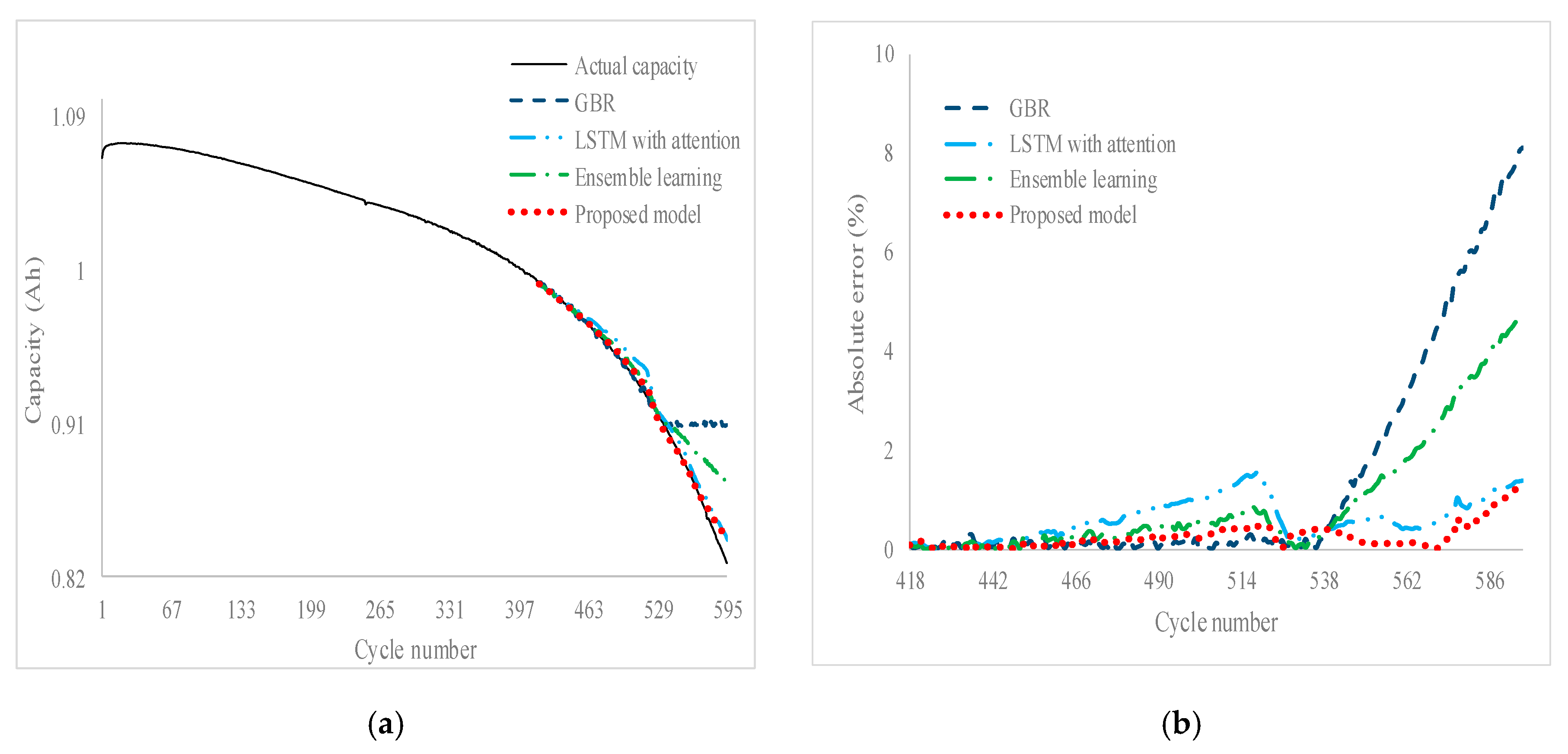
Table 3 shows the capacity degradation predictions of different models. The results indicate that the proposed model outperforms the other two single models and the conventional ensemble learning model. For example, on cell #2_5, the RMSE values of the GBR, LSTM with attention, conventional ensemble learning, and proposed models are 0.0290, 0.0121, 0.0198, and 0.0047, respectively. LSTM with an attention model provides the second-best value for the prediction of lithium–ion capacity trends. Due to the worst prediction result of the GBR model, the performance of the conventional ensemble learning model becomes worse than that of the LSTM with the attention model. As a result, the conventional ensemble learning model does not necessarily guarantee that its prediction results will be better than a single model. For further clarification, Figure 3 and Figure 4 show the prediction performance of different models for cells #2_11 and #2_12, respectively.
Although the proposed model provides better prediction performance, it has a longer computation time than other models, as shown in Table 4. This is the limitation of our proposed model. The computation time of the LSTM with the attention model is the lowest; however, the time required to find the optimal parameters of the LSTM with the attention model will take several hours, depending on the number of iterations in the DE algorithm.
The MC dropout method is used for variance estimation to construct a prediction interval. The proposed model was run 100 times with random dropout, which will produce different output values. We can calculate the mean and variance of the prediction results from these different output values, and then use the conventional formula to construct the prediction interval. Figure 5 shows the prediction interval of the proposed model on 2_11 and 2_12 cells at a 95% confidence level, where LB is the lower boundary, and UB is the upper boundary. The narrow width of the interval indicates that the prediction result is more reliable and credible. The prediction uncertainty increases when the prediction point is far from the starting cycle of test data.
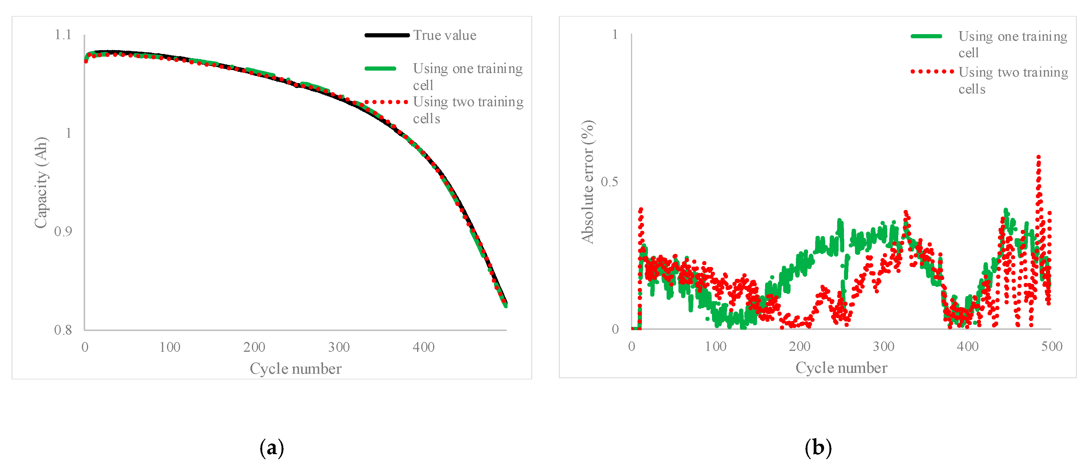
In the second experiment, one or two cells were used as training data, and other cells were used as test data to verify the proposed model. The training data can be one cell or two cells. Table 5 lists the performances of different models. The average MAPE values of GBR, LSTM with attention, and the proposed model are 1.2734, 0.9029, and 0.7294. The results show that the proposed model performs better than the GBR model and the LSTM with the attention model in all cases. For the test data such as cells #3 and #2_27, two training cells can provide better predictive performance than one training cell. Figure 6 shows the prediction performance of the proposed model using one cell or two cells as training data for cell #2_27. This shows that the proposed model can accurately predict the degradation trend of lithium–ion battery capacity.
4.2. Cycle Life Prediction
The cycle life prediction of the proposed model is evaluated by using an absolute percentage error (APE), which is given by
where represents actual cycle life and represents the predicted cycle life. The lowest APE value indicates that the model has better performance. Table 6 provides the performance of the different models by the cycle life of a single cell experiment. The actual cycle life values for seven cells are given in the second column of Table 6. In addition, Table 7 shows the estimated life cycle of six cells under one cell or two cells as training data with the actual cycle life for four test cells. For cells #2_26 and #2_27, The results show that by averaging the experimental results, the model has better performance than the single model.
5. Conclusions
Our research uses an ensemble model based on stacked long short-term memory, which combines the LSTM with attention and gradient boost regression models to predict the cycle life of lithium–ion batteries. The model hyperparameters are obtained by using the DE algorithm. The performance of the proposed model is compared with a single model using single and multiple cells for training. The first experiment used data from seven cells to verify the performance of the proposed model, where 70% of the data was used for model training, and the remaining data were used for model verification. The second experiment used one cell or two cells as the training set, and other cells to verify the model’s predictive ability. In most cases, the comparison results verify that the proposed model is superior to the single model in predicting the capacity decline trend. In the first experiment, the maximum APE value for predicting cycle life is 0.4504. In the second experiment, the average APE values of GBR, LSTM with attention, and the proposed model are 28.6580, 1.7813, and 1.5789, respectively. These results show that the proposed model has a better cycle life prediction performance than other models. In addition, the prediction variance of the model can be obtained using the MC dropout technique, which can provide prediction uncertainty. From the analysis results, we conclude that the proposed model can provide more accurate and reliable prediction results; however, the calculation time required for the ensemble model is longer than that of the single model.
In the future, the capacity degradation and cycle life prediction of other ensemble learning models in different types of lithium–ion batteries are worth investigating. In addition, the number of single models used in ensemble models can be increased to more than five. In Table 5, we found that two cells as training data provide better prediction accuracy than one cell; however, this result comes from a small experiment. Further large-scale experimental data analysis is worthy of studying the results of transfer learning.
Author Contributions
F.-K.W. conceived the original ideas; C.-Y.H. and T.M. wrote R code and analyzed the data under advice from F.-K.W.; C.-Y.H. and T.M. wrote the paper under guidance from F.-K.W. All authors have read and agreed to the published version of the manuscript.
Funding
This research was funded by The Ministry of Science and Technology in Taiwan under Grant No. MOST-107-2221-E011-100-MY3.
Conflicts of Interest
The authors declare no conflict of interest.
References
- Smith, K.; Saxon, A.; Keyser, M.; Lundstrom, B.; Cao, Z.; Roc, A. Life prediction model for grid-connected Li-ion battery energy storage system. In Proceedings of the 2017 American Control Conference (ACC), Seattle, DC, USA, 24–26 May 2017; pp. 4062–4068. [Google Scholar]
- Severson, K.A.; Attia, P.M.; Jin, N.; Perkins, N.; Jiang, B.; Yang, Z.; Chen, M.H.; Aykol, M.; Herring, P.K.; Fraggedakis, D.; et al. Data-driven prediction of battery cycle life before capacity degradation. Nat. Energy 2019, 4, 383–391. [Google Scholar] [CrossRef] [Green Version]
- Liu, C.; Wang, Y.; Chen, Z. Degradation model and cycle life prediction for lithium-ion battery used in hybrid energy storage system. Energy 2019, 166, 796–806. [Google Scholar] [CrossRef]
- Harting, N.; Schenkendorf, R.; Wolff, N.; Krewer, U. State-of-health identification of lithium-ion batteries based on nonlinear frequency response analysis: First steps with machine learning. Appl. Sci. 2018, 8, 821. [Google Scholar] [CrossRef] [Green Version]
- Tan, Y.; Zhao, G. A novel state-of-health prediction method for lithium-ion batteries based on transfer learning with long short-term memory network. IEEE Trans. Ind. Electron. 2019. [Google Scholar] [CrossRef]
- Zhang, C.; Zhu, Y.; Dong, G.; Wei, J. Data-driven lithium-ion battery states estimation using neural networks and particle filtering. Int. J. Energy Res. 2019, 43, 8230–8241. [Google Scholar] [CrossRef]
- Guo, P.; Cheng, Z.; Yang, L. A data-driven remaining capacity estimation approach for lithium-ion batteries based on charging health feature extraction. J. Power Sources 2019, 412, 442–450. [Google Scholar] [CrossRef]
- Cheng, Y.; Zerhouni, N.; Lu, C. A hybrid remaining useful life prognostic method for proton exchange membrane fuel cell. Int. J. Hydro. Energy 2018, 43, 12314–21237. [Google Scholar] [CrossRef]
- Li, Z.; Wu, D.; Hu, C.; Terpenny, J. An ensemble learning-based prognostic approach with degradation-dependent weights for remaining useful life prediction. Reliab. Eng. Syst. Safe. 2019, 184, 110–122. [Google Scholar] [CrossRef]
- Javed, K.; Gouriveau, R.; Zerhouni, N.; Hissel, D. Prognostics of proton exchange membrane fuel cells stack using an ensemble of constraints based connectionist networks. J. Power Sources 2016, 324, 745–757. [Google Scholar] [CrossRef]
- Shao, M.; Zhu, X.J.; Cao, H.F.; Shen, H.F. An artificial neural network ensemble method for fault diagnosis of proton exchange membrane fuel cell system. Energy 2014, 67, 268–275. [Google Scholar] [CrossRef]
- Zhang, D.; Baraldi, P.; Cadet, C.; Yousfi-Steiner, N.; Bérenguer, C.; Zio, E. An ensemble of models for integrating dependent sources of information for the prognosis of the remaining useful life of proton exchange membrane fuel cells. Mech. Syst. Signal Process. 2019, 124, 479–501. [Google Scholar] [CrossRef] [Green Version]
- Li, Z.; Fang, H.; Yan, Y. An ensemble hybrid model with outlier detection for prediction of lithium-ion battery remaining useful life. In Proceedings of the 2019 Chinese Control and Decision Conference (CCDC), Nanchang, China, 3–5 June 2019; pp. 2630–2635. [Google Scholar]
- Zhang, Y.; Xiong, R.; He, H.; Liu, Z. A LSTM-RNN method for the lithuim-ion battery remaining useful life prediction. In Proceedings of the 2017 Prognostics and System Health Management Conference (PHM-Harbin), Harbin, China, 9–12 July 2017; pp. 1–4. [Google Scholar]
- Chen, Z.; Sun, M.; Shu, X.; Xiao, R.; Shen, J. Online state of health estimation for lithium-ion batteries based on support vector machine. Appl. Sci. 2018, 8, 925. [Google Scholar] [CrossRef] [Green Version]
- Wang, F.K.; Mamo, T. A hybrid model based on support vector regression and differential evolution for remaining useful lifetime prediction of lithium-ion batteries. J. Power Sources 2018, 401, 49–54. [Google Scholar] [CrossRef]
- Hochreiter, S.; Schmidhuber, J. Long short-term memory. Neural Comput. 1997, 9, 1735–1780. [Google Scholar] [CrossRef] [PubMed]
- Lee, S.; Lee, Y.S.; Son, Y. Forecasting daily temperatures with different time interval data using deep neural networks. Appl. Sci. 2020, 10, 1609. [Google Scholar] [CrossRef] [Green Version]
- Wang, C.; Lu, N.; Wang, S.; Cheng, Y.; Jiang, B. Dynamic long short-term memory neural-network-based indirect remaining-useful-life prognosis for satellite lithium-ion battery. Appl. Sci. 2018, 8, 2078. [Google Scholar] [CrossRef] [Green Version]
- Ma, R.; Yang, T.; Breaz, E.; Li, Z.; Briois, P.; Gao, F. Data-driven proton exchange membrane fuel cell degradation predication through deep learning method. Appl. Energy 2018, 231, 102–115. [Google Scholar] [CrossRef]
- Kim, S.; Kang, M. Financial series prediction using attention LSTM. arXiv 2019, arXiv:1902.10877. [Google Scholar]
- Liu, J.; Wang, G.; Duan, L.Y.; Abdiyeva, K.; Kot, A.C. Skeleton-based human action recognition with global context-aware attention LSTM networks. IEEE Trans. Image Process. 2017, 27, 1586–1599. [Google Scholar] [CrossRef] [Green Version]
- Ran, X.; Shan, Z.; Fang, Y.; Lin, C. An LSTM-based method with attention mechanism for travel time prediction. Sensors 2019, 19, 861. [Google Scholar] [CrossRef] [Green Version]
- Raffel, C.; Ellis, D.P. Feed-forward networks with attention can solve some long-term memory problems. arXiv 2015, arXiv:1512.08756. [Google Scholar]
- Breiman, L. Random forests. Mach. Learn. 2001, 45, 5–32. [Google Scholar] [CrossRef] [Green Version]
- Friedman, J.H. Stochastic gradient boosting. Comput. Stat. Data An. 2002, 38, 367–378. [Google Scholar] [CrossRef]
- Ridgeway, G. Generalized boosted models: A guide to the GBM package. Update 2007, 1–15. [Google Scholar]
- Storn, R.; Price, K. Differential evolution-a simple and efficient heuristic for global optimization over continuous spaces. J. Glob. Optim. 1997, 11, 341–359. [Google Scholar] [CrossRef]
- Price, K.; Storn, R.M.; Lampinen, J.A. Differential Evolution: A Practical Approach to Global Optimization; Springer Science & Business Media: Berlin, Germany, 2006. [Google Scholar]
- Mullen, K.; Ardia, D.; Gil, D.L.; Windover, D.; Cline, J. DEoptim: An R package for global optimization by differential evolution. J. Stat. Softw. 2011, 40, 1–26. [Google Scholar] [CrossRef] [Green Version]
- Gal, Y.; Ghahramani, Z. Dropout as a bayesian approximation: Representing model uncertainty in deep learning. In Proceedings of the International Conference on Machine Learning 2016, New York City, NY, USA, 19–24 June 2016; pp. 1050–1059. [Google Scholar]

Figure 2.
The flowchart of the proposed model.
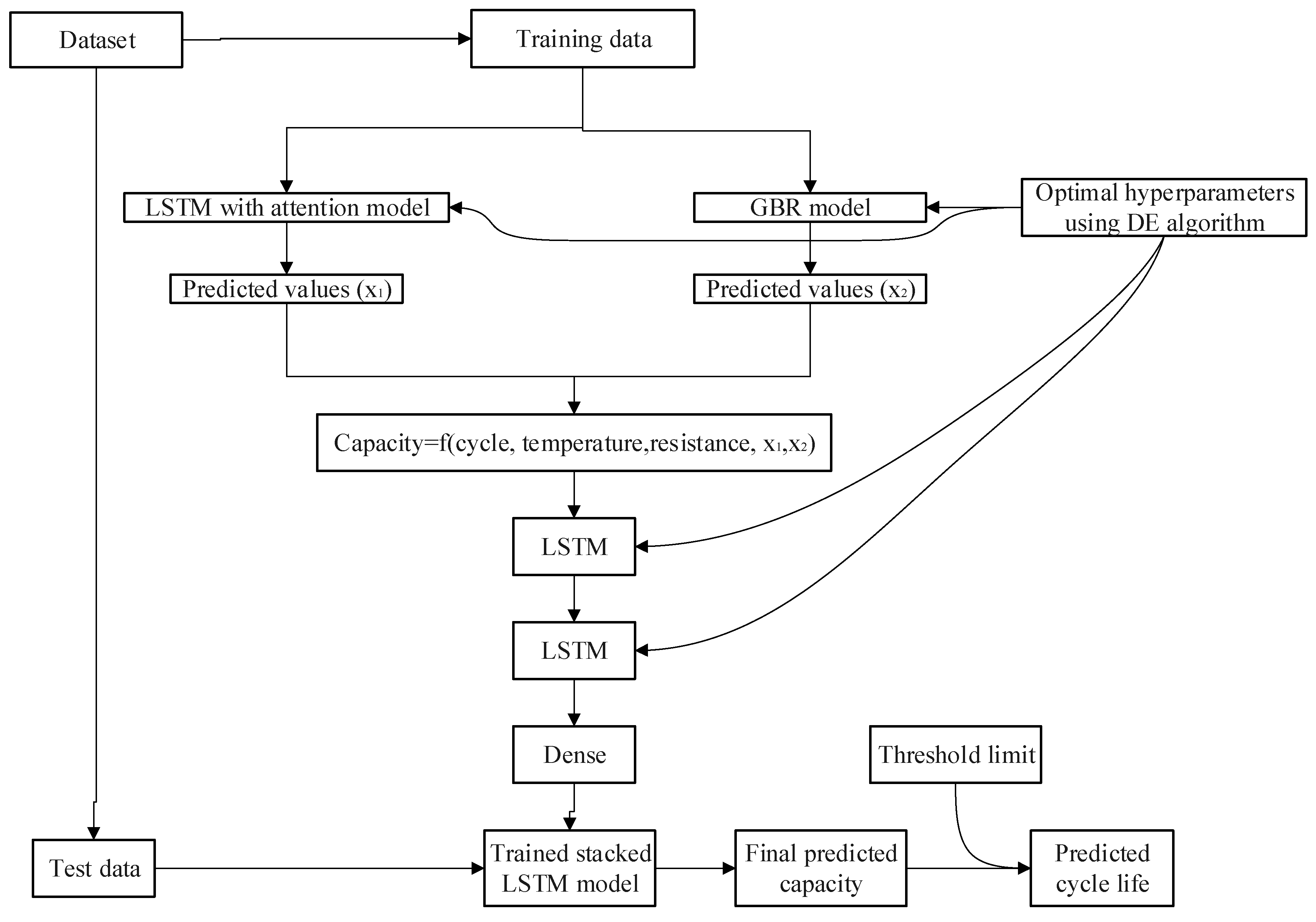
Figure 3.
Prediction performance of different models on cell #2_11 cell: (a) prediction performance and (b) absolute error.
Figure 3.
Prediction performance of different models on cell #2_11 cell: (a) prediction performance and (b) absolute error.

Figure 4.
Prediction performance of different models on cell #2_12: (a) prediction performance and (b) absolute error.
Figure 4.
Prediction performance of different models on cell #2_12: (a) prediction performance and (b) absolute error.
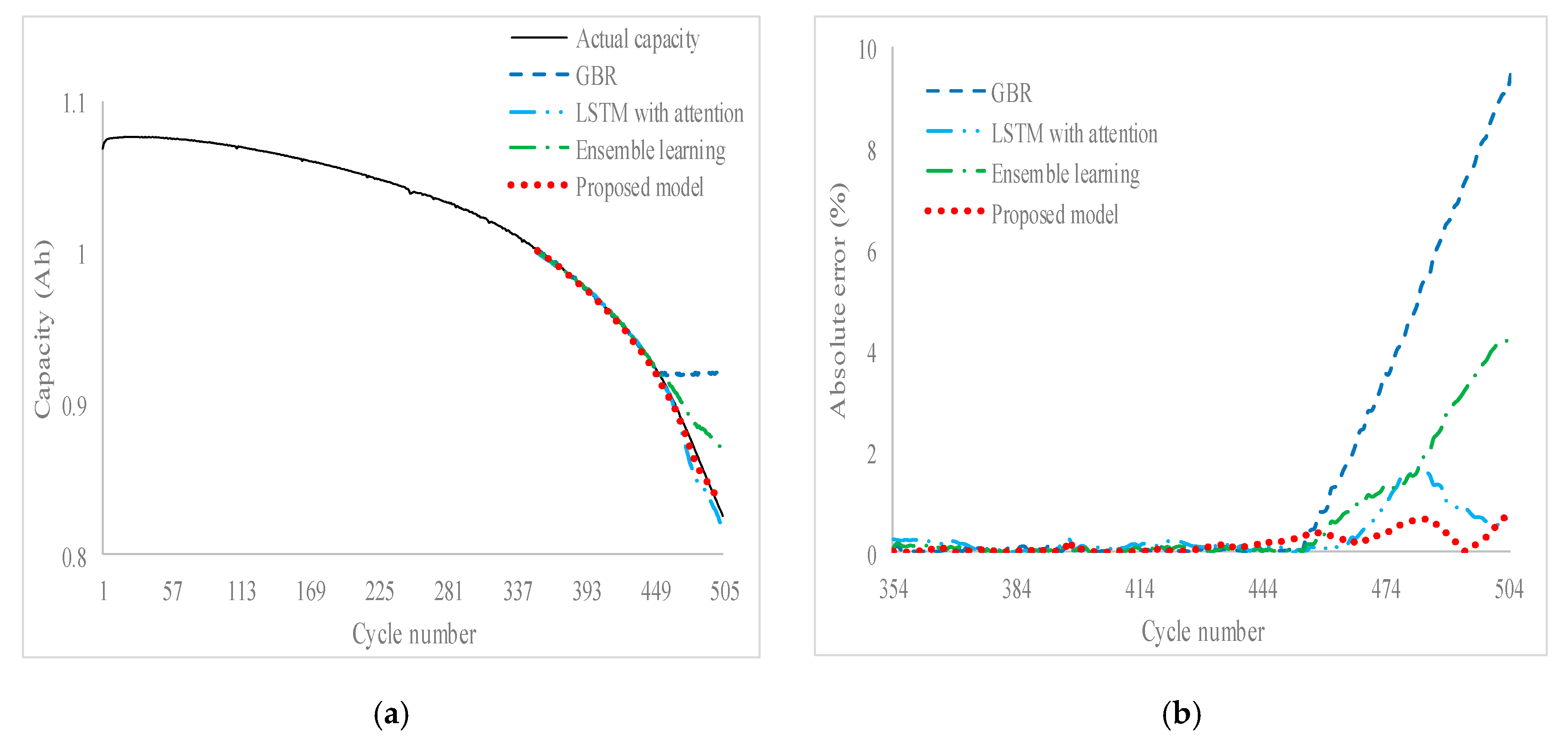
Figure 5.
Proposed model prediction intervals: (a) cell #2_11 cell and (b) cell #2_12.

Figure 6.
The prediction performance of the proposed model using one cell or two cells as training data for cell 2_27: (a) predicted capacity and (b) absolute prediction error.
Figure 6.
The prediction performance of the proposed model using one cell or two cells as training data for cell 2_27: (a) predicted capacity and (b) absolute prediction error.

Table 1.
Summary of the thirteen cells.
| Cell Barcode | Cell | Cycle Life | Charging Policy | Experiment |
|---|---|---|---|---|
| EL150800460655 | 2_5 | 444 | 3.6C (22%)—5.5C | 1 |
| EL150800460635 | 2_6 | 480 | 3.6C (2%)—4.85C | 1 |
| EL150800460208 | 2_11 | 483 | 4C 40%)—6C | 1 |
| EL150800460449 | 2_12 | 485 | 4C (4%)—4.85C | 1 |
| EL150800460480 | 2_14 | 487 | 4.4C (47%)—5.5C | 1 |
| EL150800460603 | 2_18 | 513 | 4.65C (44%)—5C | 1 |
| EL150800460501 | 2_19 | 527 | 4.65C (19%)—4.85C | 1 |
| EL150800460514 | 1 | 1852 | 3.6C (80%)—3.6C | 2 |
| EL150800460486 | 2 | 2160 | 3.6C (80%)—3.6C | 2 |
| EL150800460623 | 3 | 2237 | 3.6C (80%)—3.6C | 2 |
| EL150800460597 | 2_25 | 495 | 4.8C (80%)—4.8C | 2 |
| EL150800463611 | 2_26 | 461 | 4.8C (80%)—4.8C | 2 |
| EL150800460596 | 2_27 | 471 | 4.8C (80%)—4.8C | 2 |
Table 2.
Optimal parameters of long short-term memory (LSTM) with attention model and stacked long short-term memory (SLSTM) model.
Table 2.
Optimal parameters of long short-term memory (LSTM) with attention model and stacked long short-term memory (SLSTM) model.
| Models | Cells | Lookback | Batch Size | Neuro | Steps per Epoch | Epochs |
|---|---|---|---|---|---|---|
| LSTM with attention | 2_5 | 8 | 21 | 15 | 45 | 59 |
| 2_6 | 8 | 27 | 38 | 20 | 41 | |
| 2_11 | 9 | 23 | 26 | 58 | 65 | |
| 2_12 | 7 | 23 | 20 | 58 | 55 | |
| 2_14 | 9 | 26 | 20 | 54 | 41 | |
| 2_18 | 9 | 23 | 16 | 57 | 32 | |
| 2_19 | 9 | 22 | 16 | 31 | 31 | |
| Proposed model (SLSTM) | 2_5 | 9 | 23 | 77 | 54 | 59 |
| 2_6 | 7 | 23 | 53 | 57 | 31 | |
| 2_11 | 5 | 21 | 72 | 55 | 57 | |
| 2_12 | 7 | 23 | 53 | 57 | 31 | |
| 2_14 | 9 | 26 | 17 | 54 | 51 | |
| 2_18 | 7 | 23 | 53 | 57 | 31 | |
| 2_19 | 9 | 28 | 56 | 58 | 70 |
Table 3.
Capacity degradation prediction of different models.
| Cells | GBR Model | LSTM with Attention | Ensemble Learning | Proposed Model | ||||
|---|---|---|---|---|---|---|---|---|
| MAPE | RMSE | MAPE | RMSE | MAPE | RMSE | MAPE | RMSE | |
| 2_5 | 1.7129 | 0.0290 | 0.9936 | 0.0121 | 1.2959 | 0.0198 | 0.3049 | 0.0047 |
| 2_6 | 1.9143 | 0.0319 | 0.5822 | 0.0068 | 1.1689 | 0.0182 | 0.1669 | 0.0024 |
| 2_11 | 1.5997 | 0.0266 | 0.7603 | 0.0082 | 1.1079 | 0.0158 | 0.2782 | 0.0036 |
| 2_12 | 1.8556 | 0.0314 | 0.3497 | 0.0046 | 0.8109 | 0.0136 | 0.1912 | 0.0026 |
| 2_14 | 1.7974 | 0.0291 | 0.8646 | 0.0097 | 1.2588 | 0.0162 | 0.2681 | 0.0041 |
| 2_18 | 1.7245 | 0.0287 | 0.3201 | 0.0042 | 0.8357 | 0.0129 | 0.1959 | 0.0025 |
| 2_19 | 1.5872 | 0.0252 | 0.9389 | 0.0124 | 1.1991 | 0.0183 | 0.2656 | 0.0045 |
Table 4.
The computation time of different models (in seconds).
| Cells | GBR Model | LSTM with Attention | Ensemble Learning | Proposed Model |
|---|---|---|---|---|
| 2_5 | 78.6 | 65.4 | 141.0 | 261.6 |
| 2_6 | 69.6 | 23.7 | 94.8 | 150.0 |
| 2_11 | 82.2 | 88.8 | 173.4 | 269.4 |
| 2_12 | 77.4 | 71.4 | 150.6 | 205.2 |
| 2_14 | 80.4 | 51.4 | 134.4 | 210.0 |
| 2_18 | 78.6 | 43.3 | 121.8 | 177.0 |
| 2_19 | 64.8 | 25.6 | 90.6 | 225.6 |
Table 5.
The prediction performance of different models using one cell or two cells as training data.
Table 5.
The prediction performance of different models using one cell or two cells as training data.
| Training Data | Test Data | GBR Model | LSTM with Attention | Proposed Model | |||
|---|---|---|---|---|---|---|---|
| MAPE | RMSE | MAPE | RMSE | MAPE | RMSE | ||
| 1 | 2 | 2.0698 | 0.0257 | 1.9664 | 0.0241 | 1.7802 | 0.0219 |
| 3 | 2.0254 | 0.0254 | 1.9340 | 0.0239 | 1.7519 | 0.0217 | |
| 1 & 2 | 3 | 0.1297 | 0.0022 | 0.0406 | 0.0017 | 0.0330 | 0.0019 |
| 2_25 | 2_26 | 1.1099 | 0.0194 | 0.5025 | 0.0188 | 0.2467 | 0.0118 |
| 2_27 | 1.4351 | 0.0220 | 0.5599 | 0.0194 | 0.3058 | 0.0123 | |
| 2_25 & 2_26 | 2_27 | 0.8704 | 0.0113 | 0.4139 | 0.0144 | 0.2585 | 0.0128 |
| Average | 1.2734 | 0.0177 | 0.9029 | 0.0171 | 0.7294 | 0.0137 | |
Table 6.
The cycle life prediction results of different models using 70% of the total data as training data.
Table 6.
The cycle life prediction results of different models using 70% of the total data as training data.
| Cells | ACL | GBR Model | LSTM with Attention | Ensemble Learning | Proposed Model | ||||
|---|---|---|---|---|---|---|---|---|---|
| PCL | APE | PCL | APE | PCL | APE | PCL | APE | ||
| 2_5 | 444 | 471 | 6.0811 | 453 | 2.0270 | 471 | 6.0811 | 446 | 0.4504 |
| 2_6 | 480 | 507 | 5.6250 | 484 | 0.8333 | 507 | 5.6250 | 479 | 0.2083 |
| 2_11 | 561 | 596 | 6.2389 | 565 | 0.7130 | 589 | 4.9911 | 561 | 0.0000 |
| 2_12 | 477 | 505 | 5.8700 | 474 | 0.6289 | 492 | 3.1447 | 475 | 0.4192 |
| 2_14 | 483 | 520 | 7.6605 | 486 | 0.6211 | 505 | 4.5549 | 481 | 0.4141 |
| 2_18 | 494 | 525 | 6.2753 | 490 | 0.8097 | 509 | 3.0364 | 492 | 0.4049 |
| 2_19 | 487 | 523 | 7.3922 | 497 | 2.0534 | 521 | 6.9815 | 486 | 0.2053 |
Table 7.
The cycle life prediction results of different models using one cell or two cells as training data.
Table 7.
The cycle life prediction results of different models using one cell or two cells as training data.
| Training Data | Test Data | ACL | GBR Model | STM with Attention | Proposed Model | |||
|---|---|---|---|---|---|---|---|---|
| PCL | APE | PCL | APE | PCL | APE | |||
| 1 | 2 | 1145 | 338 | 70.4803 | 1177 | 2.7948 | 1177 | 2.7948 |
| 3 | 1140 | 207 | 81.8421 | 1146 | 0.5263 | 1142 | 0.1754 | |
| 1 & 2 | 3 | 1140 | 1176 | 3.1579 | 1134 | 0.5263 | 1139 | 0.0877 |
| 2_25 | 2_26 | 461 | 487 | 5.6399 | 451 | 2.1692 | 451 | 2.1692 |
| 2_27 | 471 | 498 | 5.7325 | 460 | 2.3355 | 460 | 2.3355 | |
| 2_25 & 2_26 | 2_27 | 471 | 447 | 5.0955 | 460 | 2.3355 | 462 | 1.9108 |
| Average APE | 28.6580 | 1.7813 | 1.5789 | |||||
© 2020 by the authors. Licensee MDPI, Basel, Switzerland. This article is an open access article distributed under the terms and conditions of the Creative Commons Attribution (CC BY) license (http://creativecommons.org/licenses/by/4.0/).
Share and Cite
MDPI and ACS Style
Wang, F.-K.; Huang, C.-Y.; Mamo, T. Ensemble Model Based on Stacked Long Short-Term Memory Model for Cycle Life Prediction of Lithium–Ion Batteries. Appl. Sci. 2020, 10, 3549. https://doi.org/10.3390/app10103549
AMA Style
Wang F-K, Huang C-Y, Mamo T. Ensemble Model Based on Stacked Long Short-Term Memory Model for Cycle Life Prediction of Lithium–Ion Batteries. Applied Sciences. 2020; 10(10):3549. https://doi.org/10.3390/app10103549
Chicago/Turabian StyleWang, Fu-Kwun, Chang-Yi Huang, and Tadele Mamo. 2020. "Ensemble Model Based on Stacked Long Short-Term Memory Model for Cycle Life Prediction of Lithium–Ion Batteries" Applied Sciences 10, no. 10: 3549. https://doi.org/10.3390/app10103549
Note that from the first issue of 2016, this journal uses article numbers instead of page numbers. See further details here.