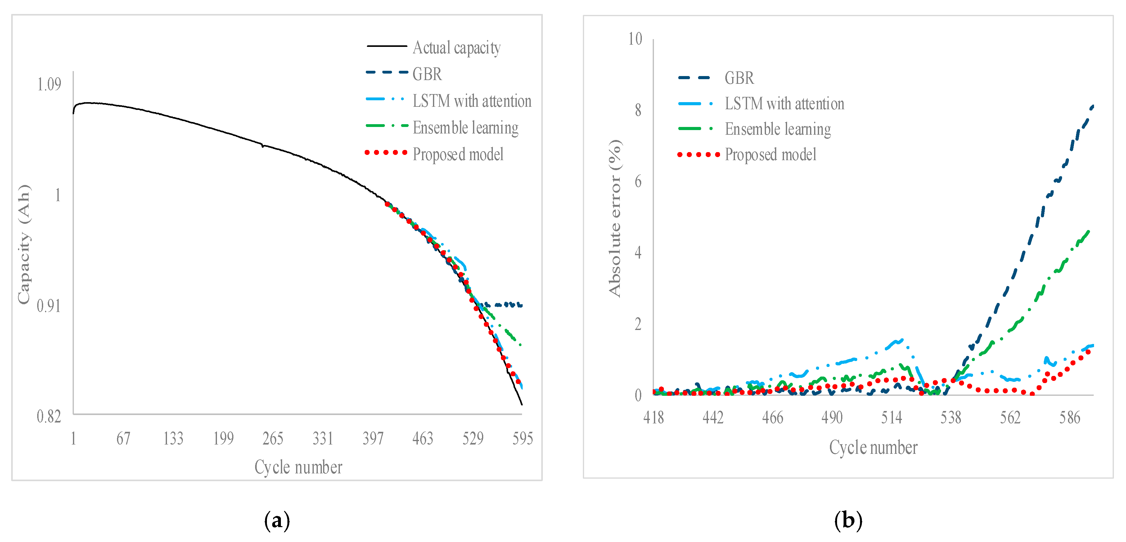
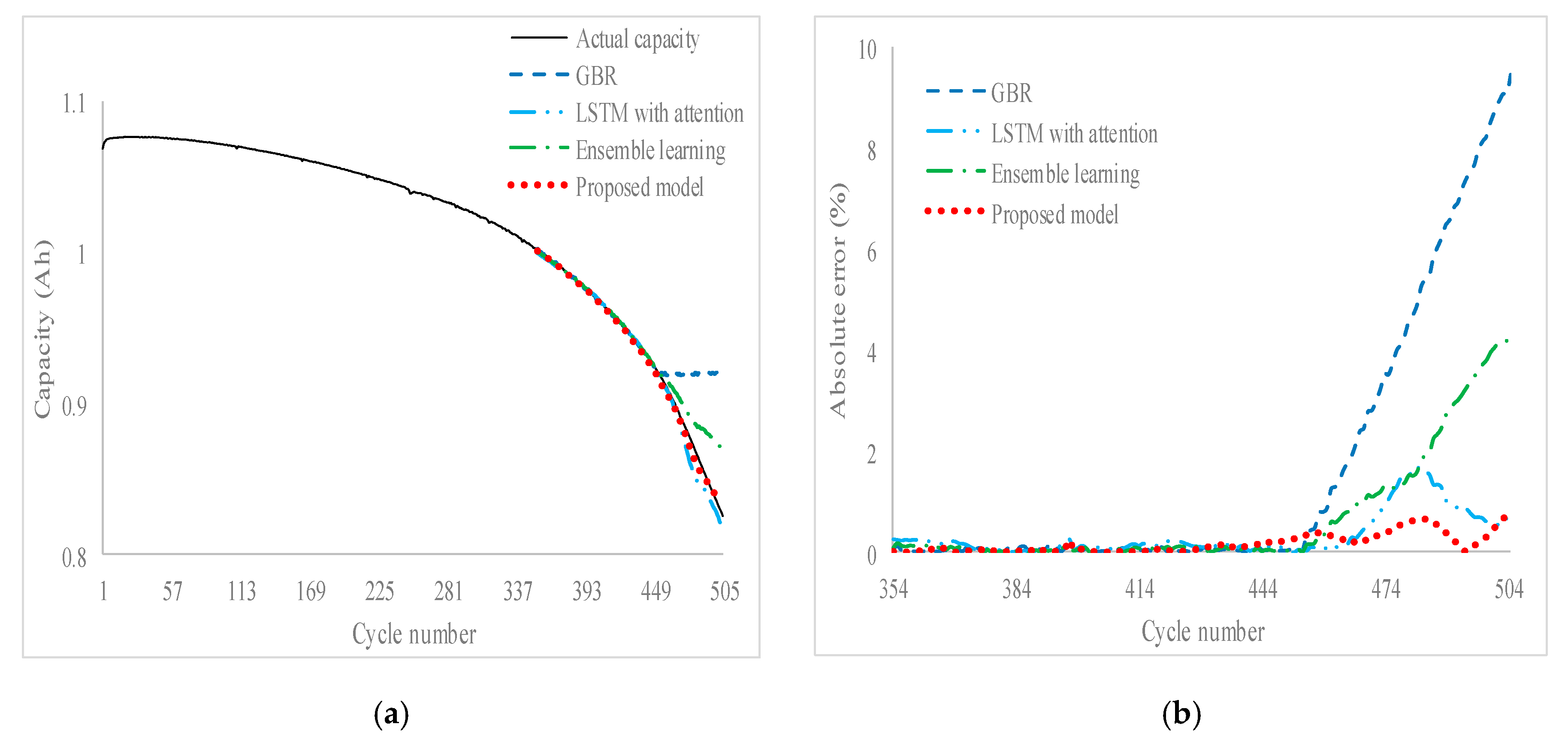
In this study, we propose an ensemble model based on the SLSTM model for cycle life prediction. The ensemble model is based on two models, LSTM with attention and GBR models, which are introduced in this subsection.
3.1. LSTM with an Attention Mechanism
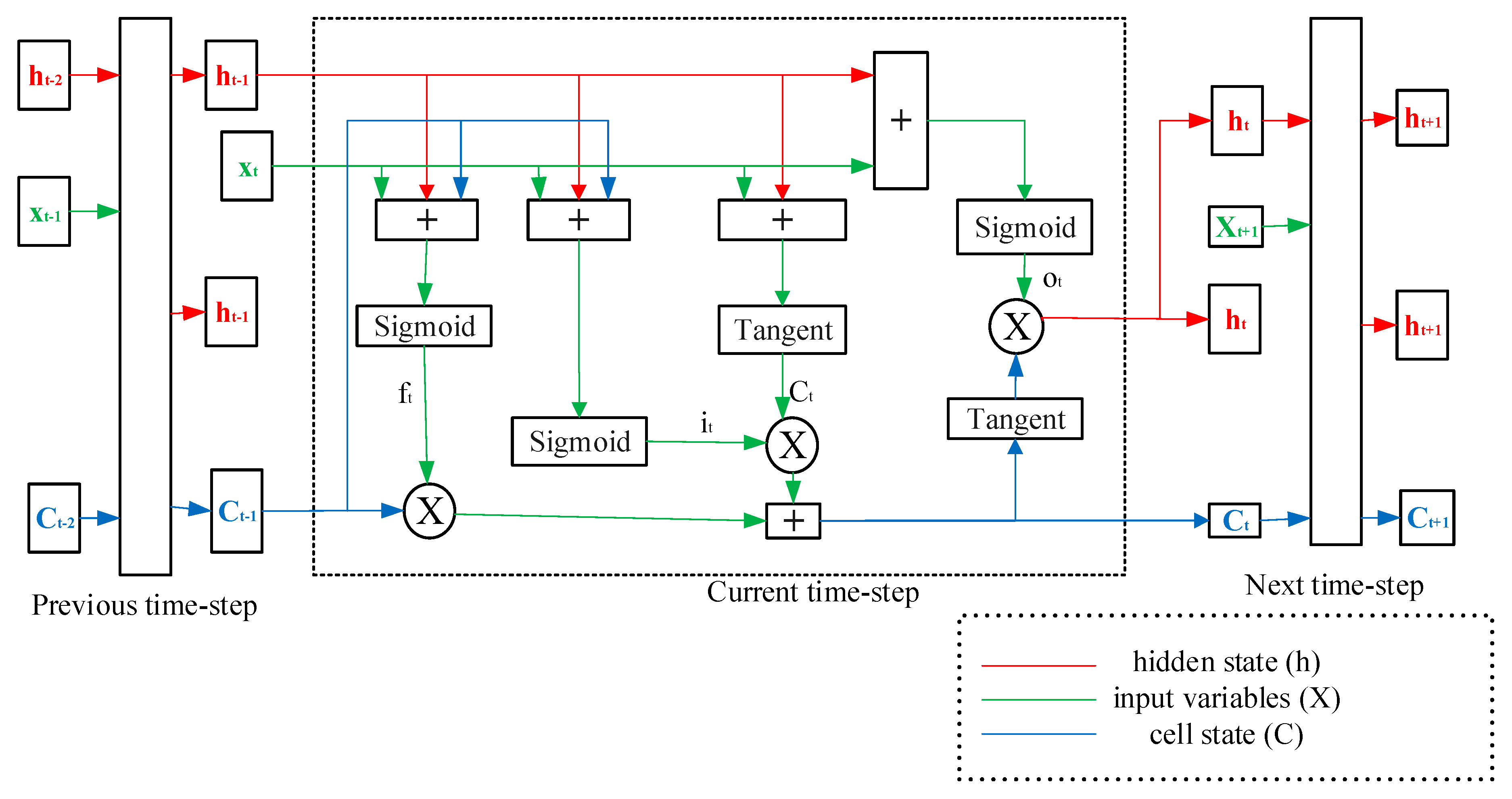
Although the standard recurrent neural network is an extension of the conventional feed-forward neural network, it has the problem of gradient vanishing or explosion. LSTM was developed to solve these problems and achieve excellent performance. It has unique memory and forgetting modes and can be flexibly adapted to the timing characteristics of network learning tasks. The units of the LSTM model includes a forget gate, input gate, and output gate [
17,
18]. The forget gate is designed to determine whether it needs to be discarded from the cell state. The input gate is designed to determine whether new information should be stored in the cell state. The output gate is designed to determine what information will be transferred from the cell state to the current hidden layer data. These gating units are derived by
where
is the sigmoid function to keep the output value between 0 and 1;
ht−1 and
Xt are previous layer data and the current input layer data;
are the input weight, the recurrent weight, and the bias of a forget gate.
where
are the input weight, the recurrent weight, and the bias of an input gate. A tanh layer is chosen to form the new memory as
where
are the input weight, the recurrent weight, and the bias of a new memory. Then, the cell state is updated by
.
where
are the input weight, the recurrent weight, and the bias of an output gate. Finally, we multiply it by the output of the sigmoid gate as
.
Figure 1 shows the architecture of the LSTM cell.
Recently, the attention mechanism is usually used to analyze images and time-series data. Compared with other ordinary deep learning models, combining attention with LSTM can obtain better results. Note that the attention layer only helps to select the output of earlier layers that are critical to each subsequent stage of the model. It allows the network to focus on specific information selectively. It is accomplished by building a neural network focused on appropriate tasks. Detailed information on the attention-based LSTM model can be found in [
21,
22,
23,
24]. In this study, the attention-based LSTM model is used as a single model. The best model parameters are obtained from the DE algorithm.
3.2. Gradient Boosted Regression
Gradient boosting is a useful machine learning model that can obtain accurate results in various practical tasks. It focuses on the errors caused by each step iteratively until the weak learners are combined by finding suitable strong learners as the sum of consecutive weak learners [
25,
26,
27]. The boosting iteration can be based on functional gradient descent. Let S =
be samples. A function
is used to predict values based on the local loss function
. We minimize the expected value of the loss function to obtain the approximate value
of the function
f(
x). GBR follows the regularization-method based on shrinkage and updates in each corresponding area as follows:
where
is called shrinkage to control the learning rate of the procedure and
is the number of leaves of
defined by the rectangular regions
. The coefficients
of a new tree can be fitted by retaining the leaves rectangles
of
as
. Parameters such as shrinkage (
v), number of trees (
t), number of leaves (
), bag fraction, and interaction depth need to be determined by using the DE algorithm. The ratio of bags is the observed score of the training data, which is randomly selected to generate the next tree.
3.3. Propose Model
Figure 2 illustrates a novel framework for cycle life prediction using an ensemble model. In the first level, two machine learning models, such as LSTM with attention and GBR models, are used to generate predictions. These predicted values are used as input features for the final prediction with actual features. In the second level, the SLSTM model with a sliding window method is used to predict the final predicted value. All hyperparameters of each model are derived using the DE algorithm. The detail of the DE algorithm can be found in [
28,
29,
30]. For example, five parameters need to be determined in advance, such as lookback, batch size, neuro, steps per epochs, and epochs in the LSTM model. The following steps can obtain the best hyperparameters.
Step 1. Extract the features such as cycle, capacity, internal resistance, and average temperature.
Step 2. Use mean absolute percentage error (MAPE) as the fitness function, which is obtained by
where
is the actual capacity at cycle
t,
is the predicted capacity at cycle
t, and
n is the prediction length.
Step 3. Select the range of LSTM and GBR hyperparameters, and use the specified model to calculate the MAPE value.
Step 4. Decide the values of DE algorithms such as NP, CR, and F, which are 50, 0.9, and 0.8, respectively, in this study.
Step 5. Output the best value. For example, the optimal values for the lookback, batch size, neuro, steps per epoch, and epochs of the proposed model in cell 2_5 are 8, 21, 15, 45, and 59, respectively.
The LSTM model should include dropout parameters to reduce overfitting and enhance model performance. Dropout is a regularization method. In this method, the cyclic connection with the input of the LSTM cell may not be excluded from the activation and weight update in network training. That is to say, two parameters (such as dropout and recursive dropout) are used for linear transformation of the recursive state. Therefore, the Monte Carlo (MC) dropout technique is used to obtain the variance and bias of the proposed model, and the sliding window method is used to construct its prediction interval. Converting a conventional network to a Bayesian network through MC dropout is as simple as using the dropout technique for each layer during training and testing. It is equivalent to sampling from the Bernoulli distribution and provides predictive stability across samples [
31]. The idea is to run the model several times with random dropout, which will produce different output values. Then, we can calculate the empirical mean and variance of the output to obtain the prediction interval for each time step. The sliding window is a temporary approximation of the actual value of the time-series data. The window and segment sizes will increase until a smaller error approximation is reached. After selecting the first segment, we select the next segment from the end of the first segment; repeat the process until all time-series data are segmented.


