Development of A Linear Delta Robot with Three Horizontal-Axial Pneumatic Actuators for 3-DOF Trajectory Tracking


1
Department of Mechanical and Electro-Mechanical Engineering, Tamkang University, New Taipei City 251301, Taiwan
2
Department of Electrical Engineering, National Taiwan Normal University, Taipei City 106308, Taiwan
3
Department of Mechanical Engineering, National Chung Hsing University, Taichung City 402204, Taiwan
*
Author to whom correspondence should be addressed.
Appl. Sci. 2020, 10(10), 3526; https://doi.org/10.3390/app10103526
Submission received: 28 March 2020
/
Revised: 27 April 2020
/
Accepted: 18 May 2020
/
Published: 20 May 2020
(This article belongs to the Special Issue Applications of Intelligent Control Methods in Mechatronic Systems)
Abstract
:This paper focuses on developing a pneumatic-driven and horizontal-structure linear delta robot (PH-LDR) and increasing its trajectory tracking performance on the three-degrees-of-freedom (3-DOF) space. With the investigation of inverse and forward kinematics, the parallel mechanism of PH-LDR is designed by using three high-power and low-cost rod-less pneumatic actuators (PAs) to track 3-DOF motion, and this has a horizontal structure to enlarge the workspace. Since the PH-LDR features nonlinear coupling among its three axes and is disturbed by the three high-nonlinear rod-less PAs, the tracking control performance is significantly decreased, subject to uncertain nonlinearity and parametric uncertainty. Therefore, a fuzzy-PID controller is used to achieve highly accurate 3-DOF trajectory tracking, and furthermore, this study exploits neural networks (NNs) to pre-compensate the impacts arising from the compressibility of air and temperature change. The control system for the PH-LDR also features an embedded controller that allows real-time control. Experimental demonstration verifies the developed PH-LDR with the proposed controller, and the dynamic tracking accuracy in 3-DOF trajectory can be achieved.

1. Introduction
Linear delta robots (LDRs) for industrial applications are superior to series manipulators, because they have a large carrying capacity and are highly precise and fast [1,2], so they are widely used for assembly detection, pick-and-place, positioning, and packaging [3]. They are constructed using multiple independent closed-loop mechanisms, each of which has an arm that connects a fixed base to a moving platform. LDRs require three linear actuators to drive the arms and to translate one-dimensional linear motion into three-degrees-of-freedom (3-DOF) movements. Linear actuators can be installed on or near to a fixed base, so that most LDRs use lightweight material for the arms and have a high rigidity-to-weight ratio. LDRs also feature excellent positioning accuracy, because the position error from one single closed-loop kinematic chain is spread among the other chains. However, LDRs have some intrinsic drawbacks, such as a small workspace and complicated kinematics, but there has been increased demand for them in recent years.
Pneumatic actuators (PAs) are low-cost and widely used devices for manufacturing. They use compressed air as the operating fluid to push a piston and produce linear movement for payloads [4,5,6]. PAs are highly suited to industrial environments, because they are clean, safe, and easier to maintain and have a high power-to-weight ratio. However, PAs are less accurate in terms of position control and less versatile and flexible for engineering applications than electrical motors with the same power, due to the compressibility of air, air leakage, a low natural frequency and high nonlinearity. Despite these inherent drawbacks, PA-driven facilities are still commonly used in manufacturing.
Milutinovic et al. [7] presented three different LDRs with actuated arms at specific angles to each other: a vertical type, a tri-pyramid type and a horizontal type. For a specific sensitivity, proper design for LDRs can fulfil a larger workspace, but cause more difficult control problems in real time, because of the multi-input and multi-output system dynamics involving various nonlinearities and coupling effects. Choi et al. [8] presented a hybrid serial-parallel pneumatic-driven robot with a high ratio of strength-to-moving-weight for mounting window glass and fixing pixels. Chiang et al. [9] developed a pneumatic-driven LDR with three pneumatic actuators on three vertical axes at 120 degrees to each other, to achieve complex 3-DOF motion control. Furthermore, Chiang et al. [10] developed a three-axial tripod-type pneumatic parallel LDR. A geometric approach was used to derive the kinematic model and drive the LDR in a 3-DOF space with an acceptable output tracking error. In [11], Andrzej et al. designed a 3-DOF tripod-type pneumatic LDR for municipal waste recycling that demonstrated excellent accuracy and repeatability in pick-and-place tasks. Lafmejani et al. [12] presented a 6-DOF pneumatic Gough–Stewart parallel robot. In order to determine an accuracy model for the 6-DOF pneumatic robot, a genetic algorithm (GA) was used to identify unknown parameters within the dynamic model of the cylinder and the proportional valve. Yan et al. [13] presented a multi-objective optimization methodology for the LDRs that optimizes dexterity, stiffness and space utilization, and showed that the methodology gives optimal solutions that are better than the results using current optimization methodology.
To address the problems of high nonlinearity, low accuracy and low robustness in LDRs, numerous control strategies have been proposed. Dongtao [14] determined the kinematic reliability and sensitivity of LDRs. Fu et al. [15] designed an LDR with three arms and showed that problems with kinematic accuracy are mostly due to U joint errors, clearances and driving errors. When the dynamics of a PA are linearized at a fixed operating point to determine the linear state equation, Liu and Bobrow [16] used a linear optimal controller to regulate the pneumatic servo system for testrobotic applications. Richer et al. [5] and Bone et al. [17] proposed a sliding mode control (SMC) to control the motion for Pas, because the SMC compensates for nonlinearities. A SMC uses a model-based approach, which can produce an unstable system which is unstable due to modeling error. To attenuate the modeling error effect in the tracking control performance, Chiang et al. [9,10,18] proposed an adaptive SMC that regulates the position of the moving platform of LDR. Lee et al. [19,20] employed a function approximation technique to determine an unknown model for PAs and increase tracking performance over time for the overall system. Despite the pervasive development of control algorithms in literature and the widespread using of PAs, the practical solution to achieve positioning accuracy and repeatability still remains an open problem in pneumatic-driven systems.
This study presents the development and implementation of a pneumatic-driven and horizontal-structure linear delta robot (PH-LDR) for industrial manufacturing that is cost-effective and highly reliable. The PH-LDR is a pneumatic-driven and horizontal-structure (PH) linear delta robot (LDR), that uses pneumatic actuators to achieve high trajectory tracking performance and reduce the cost, and which is designed as a horizontal structure to enlarge the workspace. The PH-LDR uses three rod-less PAs as the linear actuator to produce the 3-DOF motion, as well as adopting a hybrid control technique to compensate for nonlinearities and uncertainties. The rod-less PAs possess a long stroke, because unlike general pneumatic actuators, the stroke is contained within the envelope of a cylinder body. Without the need of parameter identification of the pneumatic actuating system for the controller implementation, the hybrid controller uses a simple and straightforward approach and contains two parts: a fuzzy-PID controller, as designed by using expert knowledge, to achieve the positional accuracy, and a neural network pre-compensator (NNPC), that predicts variations caused by the environmental changes such as temperature, and works with the fuzzy-PID controller. Experiments with the implemented full-scale test rig are conducted to confirm the validness of the PH-LDR for complex 3-DOF trajectory tracking problems.
The remainder of this paper is organized as follows. In Section 2, the layout of the test rig and its experimental setup are described. Furthermore, a kinematics analysis of the PH-LDR is analyzed in Section 3. The controller design for the PH-LDR is given in Section 4. Two experiments of the PH-LDR are presented in Section 5 to investigate the trajectory tracking performance. Finally, Section 6 concludes this paper.
2. Test Rig Layout
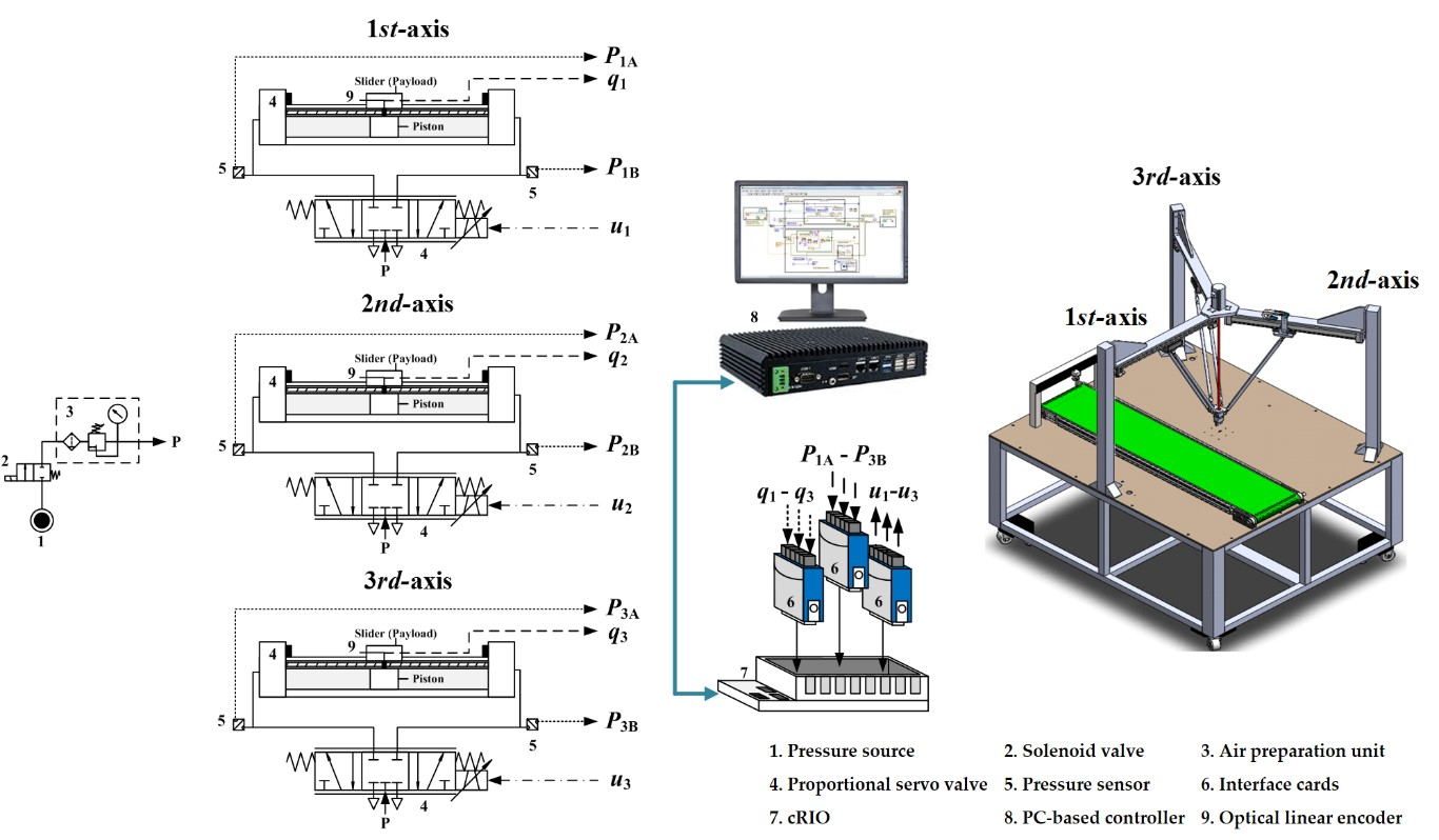
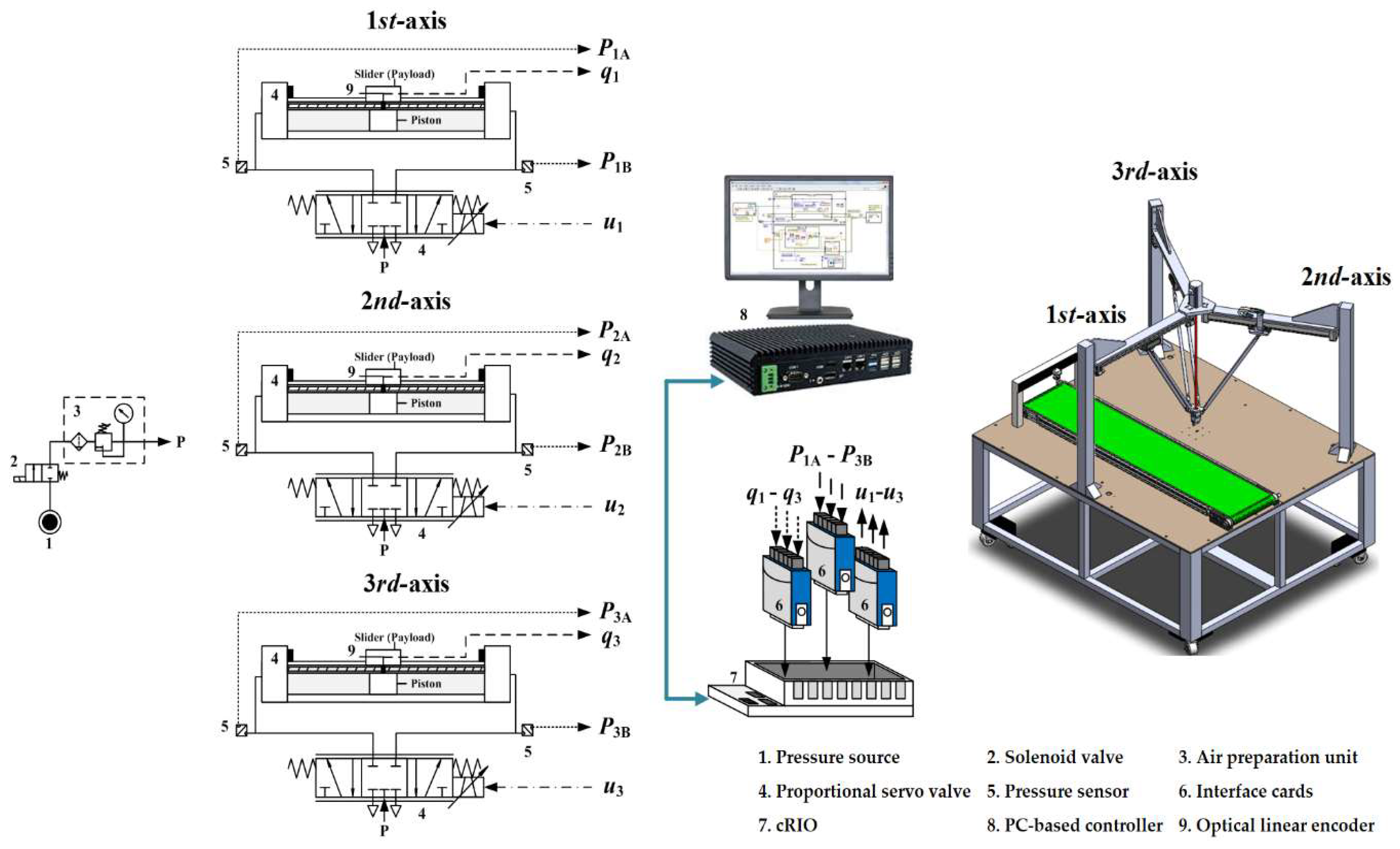
Figure 1 illustrates the test-rig layout for the PH-LDR. The PH-LDR uses three rod-less PAs that are installed under the three links at an angle of to each other. Each of the rod-less PAs produces a linear movement that drives the arms, so that the moving platform moves with 3-DOF. The rod-less PAs are Festo DGC-25-500-KF-PPV-A with a piston that has a 500 mm long stroke and a 25 mm diameter. A proportional servo valve (Festo MPYE-5-1/8-HF-010-B) controls the compressed air that flows into two chambers. The air acts on the surface of the piston to produce a rectilinear translation. The piston remains at the center of the rod-less Pas, while both of the two chambers have the same air pressure of six bars if the proportional servo valve is set to 5 V, as shown in Figure 2. Figure 1 shows that two pressure sensors (Festo SDE1) are installed on the air inlets of the cylinders to measure the pressure inside the two chambers, and three optical linear encoders with a resolution of 1μm are installed on the links to measure the position of the pistons. An embedded controller c-RIO is embedded in the control loop to achieve real-time control. It receives all measurement data via interface cards and sends an input voltage command to proportional servo valves. The interface cards include a NI-9411 digital I/O converter, a NI-9263 analog output interface card, and a NI-9215 analog input interface card. An industrial PC provides a LabVIEW integrated development environment (IDE) for developers and downloads programs into the c-RIO.
3. Analysis of Kinematics
This paper uses a vector-loop closure equation [21] for each arm to solve the solutions of the inverse kinematic model for the PH-LDR. Figure 3 shows the coordinate frames for the PH-LDR. The three arms of the PH-LDR have an identical kinematic structure. Two coordinate frames are used to analyze the kinematic model of the PH-LDR. There is a fixed Cartesian reference frame {}, for which the origin is located at the point on the fixed base. The frame {} also serves as the world coordinate. There is also a mobile Cartesian reference frame {}, for which the origin is at the center of the moving platform. are joints that are located at the center of the parallel chain of each arm and there is a pair of universal joints at its two ends and denote the location of joints on the moving platform. Three arms connect the joint and the joint and firmly connect the fixed base to the moving platform. In Figure 3, denote the actuated joint variables that are defined as the length between the point and the points . The slider moves when the PH-LDR operates, so are not constants. is the maximum value for and are equal to the maximum stroke of the rod-less PAs. Table 1 shows the geometry parameters for the PH-LDR. In this study, are defined as the joint variables; and the Cartesian variable vector represents the coordinate of the point with respect to the frame {}. The coordinates of the vector with respect to the frame {} are:
where is the unit vector along . For simplicity, the unit vector of is also defined as the vector because the orientation of {} is identical to the orientation of {} for this design. The coordinate of the vector with respect to the frame {} is:
where is the distance between and . In general, the superscript can be ignored if the vector is expressed with respect to the frame {}. In the design of the PH-LDR, the origin of the frame {} shares the plane with the origin of the frame {}, and the orientation of {} has an orientaion that is identical to the orientation of {}, so is equal to . For simplicity, therefore, is expressed as , and are expressed as .
3.1. Inverse Position Kinematics
For the inverse position kinematics, the actuated joint variables are solved for a specific position on the moving platform. In terms of Figure 3, the vector-loop closure equation for each arm is:
Substituting (1) and (2) into (3) yields:
where is the length of the kinematic chain. From Equation (4), the solution for is:
where
In Equation (5), there are two solutions for each actuator. However, only the negative square root solution satisfies the current assembly for the mechanism in which the three actuators are inclined inward from top to bottom. Thus, the inverse position kinematic equation for ith arm is:
Substituting (1), (2) and (7) into (4) yields:
As is given, the set of solutions for is:
3.2. Forward Position Kinematics
For a set of the input actuated joint variables, , the position of the moving platform, , is solved using the forward position kinemactics. In Equation (8), combining the second equation with the first equation yields:
Additionally, combining the third equation with the first equation yields:
For , the solution from Equations (10) and (11) is:
Additionally,
Substituting Equations (12) and (13) into the first equation in Equation (9) yields:
Equation (14) gives two solutions for . must be negative, because the moving platform must move under the fixed base, so the solution of is:
The unique solution of the forward position kinematic for the PH-LDR is defined in Equations (12), (13), and (15).
3.3. Velocity Analysis
If vector is the velocity vector for the sliders on the three axes and vector is the velocity vector for the moving platform, the Jacobian matrix between and is defined as [21,22]:
Differentiating Equation (8) with time yields:
Its matrix form is:
where
Additionally,
From Equations (16) and (18), we have:
where
The determinant of is calculated as:
Obviously, singularities occur for the following conditions:
Contrastingly,
Equations (24) and (25) identify the singularities at which or . There is no singularity at , because it implies that the moving platform is on the fixed base. Additionally, the initial length of the moving platform is set to 60mm so the singularity possibly occurs when the three input actuated joint variables , and reach a distance of 60mm at the same time. In our design, the length of the parallel chain of each arm for the PH-LDR is designed as 130mm and the joints are located at the center of the parallel chain of each arm, so the minimum value for the joint varibles is 65 mm. Consequently, the singularity certainly can be prevented for the operation of the PH-LDR.
4. Controller Design
The LDR is a complex MIMO system with high nonlinearities and coupling states. In general, one can design a trajectory tracking controller for the end-effector through a kinetic model or a dynamic model. Thus, nonliearities and time-varying characteristics increase when the PH-LDR carries heavyweight and high mass moment of interia, and it is so difficult to model the exact dynamics for overall control systems of the PH-LDR. Moreover, the complicated and nonlinear dynamic model make the PH-LDR auduous to design a controller to manipulate the trajectory tracking in real time, due to massive numerical computation to solve partial differential equations. The purpose of this study is to implement the PH-LDR based on the kinetic model with the intelligence based controllers, which has the self-adaptation ability to deal with system nonlinearities and parameter uncertainties.
The dynamic for the PH-LDR has two parts: a rod-less PAs dynamic and a LDR motion dynamic. The rod-less PAs dynamic model can be separated into a pneumatic servo valve dynamic model and a pneumatic cylinder dynamic model, both of which have a significant effect on the stability of the PH-LDR, due to the highly nonlinear behavior caused by the airflow and air compression. In addition, without loss of generality, the motion dynamics of the LDR can be modeled in terms of the motion equations to configure the LDR in relation to the joint torque that is exerted by the three rod-less PAs. The inverse dynamics control (IDC), which is the so-called the computed torque control [23], is a well-known control design technique for conventional LDRs. It refers to the LDR motion model and directly predicts the desired output forces or torques for actuators using a feedforward method. However, the derived PH-LDR dynamic in this study is too complicated to obtain an accurate mathematical representation, so that the IDC method is difficult to be implemented in the developed PH-LDR.
Hence, a hybrid controller is proposed, based on a simple and straightforward technique that accounts for nonlinearities and uncertainties of PH-LDR under environmental temperature changes. The designed hybrid controller consists of a fuzzy-PID controller and a NNPC. Figure 4 shows the overall control system for the PH-LDR, in which each of the three independent Fuzzy-PID + NNPC’s regulates the position of a rod-less PA. The fuzzy-PID receives the feed-back measured position and sends a control voltage to the proportional servo valve to regulate the amount of air that flows into the rod-less PA. The NNPC compensates for turnaround delay due to variations in the target, and , and variations in the temperature of the environment.
The inverse position kinematic model calculates the reference positions for the three axes using a specific 3-DOF trajectory coordinate . Accordingly, the feedback errors and the variations in the target are determined as:
Additionally,
where is the sampling time in the control loop. The outputs of define the 3-DOF position of the moving platform.
4.1. Fuzzy-PID Controller Design
In this paper, the fuzzy-PID controller uses a fuzzy inference system to determine the variations of the PID controller parameters, i.e., , for the PH-LDR. The feedback error and error change, , were adopted for yielding the online self-adjustment and . The alterations in the control parameters , and in each time step are shown as follows:
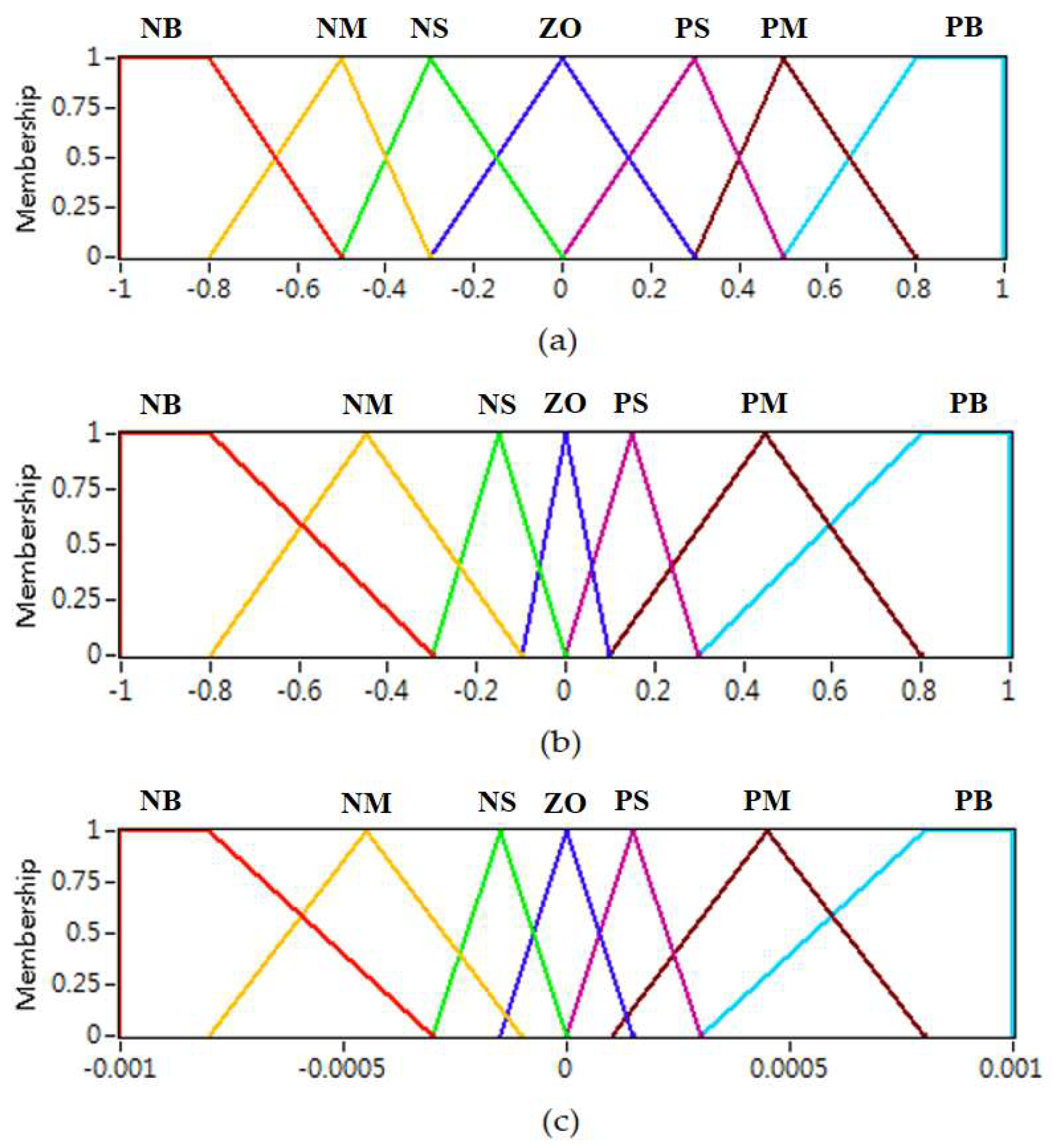
The knowledge base for a fuzzy controller consists of a rule base and membership functions. The triangle-type fuzzy membership functions for and are shown in Figure 5a, and the membership functions for are shown in Figure 5b. The fuzzy membership functions for and are shown in Figure 5c. The fuzzy subset is {NB, NM, NS, ZO, PS, PM, PB}, in which the NB, NM, NS, ZO, PS, PM, and PB stand for negative big, negative medium, negative small, zero, positive small, positive medium and positive big, respectively. These levels of each parameter were determined based on the experimental properties and characteristics of the PAs. In this paper, expert’s experience and knowledge are used to build a rule base. There are 49 rules in the fuzzy logic controller for , , and , respectively, shown in Table 2, Table 3, and Table 4, these were designed by experts. In this paper, 49 fuzzy rules are created to implement the proposed fuzzy-PID controller for the PH-LDR. The outputs of the fuzzy PID can be obtained using the Mamdani fuzzy inference and the center of area (COA) defuzzification.
4.2. NNPC Design
To prevent leaks from the high-pressure gas transmission, the gap between the rod-less PA and the slider is sealed using rubber bands. However, during the operation of PH-LDR, static friction and hysteresis between the slider and the pneumatic cylinder frequently produce a turnaround delay. A pre-compensator that adjusts the control force to account for variations in the reference position is commonly used to address turnaround delay. This paper thus formulates the pre-compensation control as a linear combination of and its rate of change, , which is expressed as:
where and are constant gains, is an offset pneumatic control voltage for the proportional servo valve, and the rate of change, , is calculated by:
When the slider moves on the rod-less pneumatic cylinder, the degree of frictional resistance to forward and backward motion is different, so the pre-compensation control is designed as:
where and denote the respective compensation gains for the slider in the forward and backward directions. When the slider moves forward, so must be greater than the median voltage. On the contrary, when the slider moves backward, so must be smaller than the median voltage. The range for the offset pneumatic control voltage in the pre-compensation control is and , since the proportional servo valve works within the interval .
When the parameters are fine-tuned, the pre-compensation control in Equation (31) is effective at dealing with the turnaround delay of each rod-less PA. However, the static friction and hysteresis in the PH-LDR exhibit highly nonlinear and coupling behavior and their values vary with time and operating temperature, so it is difficult to design accurate pre-compensation control using only the method in Equation (31). This study uses an artificial neural network (ANN) for NNPC to estimate the pre-compensation control , in which the inputs of the ANN are the environmental temperature, and , and the output of the ANN is . As shown in Figure 6, the structure of the ANN that is used for this study is a feedforward propagation network with three layers, in which the input layer has three neurons, the hidden layer has ten neurons and the output layer has one neuron. Each neuron in the ANN calculates the weighted sum of the inputs from the previous layer and then produces an output with a bias value, as written by the following:
where is the ith input node in the kth layer, is the weight between the jth node in the (k − 1)th layer and the ith node in the kth layer, is the output of the ith node in the kth layer, and is the bias of the ith node in the kth layer.
The NNPC for each rod-less PA uses the Matlab neural network toolbox to train the ANN and then the weights and bias for encoding the input-output relationship are obtained from training samples. The root-mean-square error (RMSE) is chosen as the performance function. To accelerate training speed and to avoid the problem of local minimum that is common to conventional back propagation (BP) algorithms, Levenberg–Marquardt BP is used and the training procedure will automatically terminate when the performance of generation cannot be improved. In this study, for each rod-less PA, a NNPC with a specific topology is trained and the ANN that performs best through the test set is selected. During the trajectory tracking operation of PH-LDR, the pre-compensation control for each rod-less PA is then calculated from the associated NNPC, in order to counterbalance the uncertain static friction and hysteresis. In such a case, the position regulation of rod-less Pas, even under the temperature change, can be well performed with the combination of Fuzzy-PID controller and NNPC in the feedback loop.
5. Experiments
Figure 7 shows the test-rig for the PH-LDR. Two experiments are used here to determine the feasibility of the PH-LDR. Figure 5 and Table 2, Table 3 and Table 4 respectively show the fuzzy membership functions and the fuzzy rules for the Fuzzy-PID controller. The temperature in the laboratory where the test-rig was located was between 24 °C and 28 °C. The data sets for and for the NNPC were collected between 24 °C to 28 °C, with an interval of one degree. 50% of the collected data was used to train the ANN and 50% was used for testing. During the training phase, the learning rate was set to 0.01 and the momentum coefficient was set to 0.91. The training was terminated if RMSE% < 10%, or after 10,000 iterations. In the present study, when the RMSE between the target value of and the estimated value is less than 0.1, the training procedure of ANN will be terminated. To evaluate the tracking performance for the PH-LDR, the instantaneous overall error of the moving platform is defined as:
where is defined as . The position is calculated by the forward position kinematics, as are given. , and respectively represent the tracking errors for the 1st-axis, the 2nd-axis and the 3rd-axis. It is proven in Section 3 that there are no singularities on the workspace for the PH-LDR. In this paper, the Monte Carlo method was used for the workspace analysis of the PH-LDR. The Monte Carlo method is also called the extreme limit boundary searching method, which is conducted based on the inverse solution of the kinematic location of the PH-LDR. Given all the possible workspaces of the PH-LDR, a large number of random points will be generated, and every point will be judged whether to be in the workspace or not. If it meets the constraint condition, it belongs to the workspace; if not, it shall be rejected. All the feasible points will constitute the workspace of the PH-LDR. The one from the qualified to the unqualified is just the boundary point of the workspace, and the line constituted is the boundary line. The structural parameters of the PH-LDR are shown in Table 1. The search step length of each variable was set to be 2mm. Through the Equation (9) and employment of MATLAB, the 3D stereoscopic graph of the workspace of this PH-LDR was plotted, as shown in Figure 8. The detailed steps of the Monte Carlo method for the workspace can refer to [24].
5.1. Experiment 1-Star Loop Motion Trajectory (a Two-Dimensional Motion)
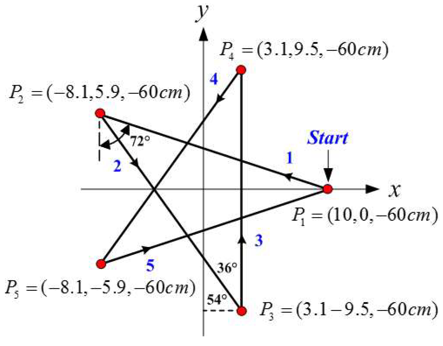
In Experiment 1, the PH-LDR tracks the plane trajectory of a star loop motion trajectory. The tracking objective is a star loop, which is composed of five oblique straight lines. The profile and the direction of movement for the trajectory are shown in Figure 9. The formulation is:
In Equation (35), is the position increment, is the x-axis trajectory, and is the y-axis trajectory of the moving platform. The actuated joint trajectories for the PH-LDR are computed by the inverse kinematics. To prevent the sliders and the shock absorber from touching at the ends of the 1st-axis, the 2nd-axis and the 3rd-axis rod-less PAs stroke during the trajectory tracking, the center position of the star motion trajectory is shifted by a bias that is larger than the amplitude of the trajectory. Initially, the moving platform moves along the fifth-order path in 3 s and the moving platform moves from the zero position to the starting point for the star motion trajectory. For segment 1 to segment 5, the platform moves along a star loop path with edges of length through five positioning points at the vertices of the star loop. The trajectory comprises six segments, which define five positioning points at the vertices of the stat: and The time that is required to travel along each of the segments 1 to 5 is 2 s.
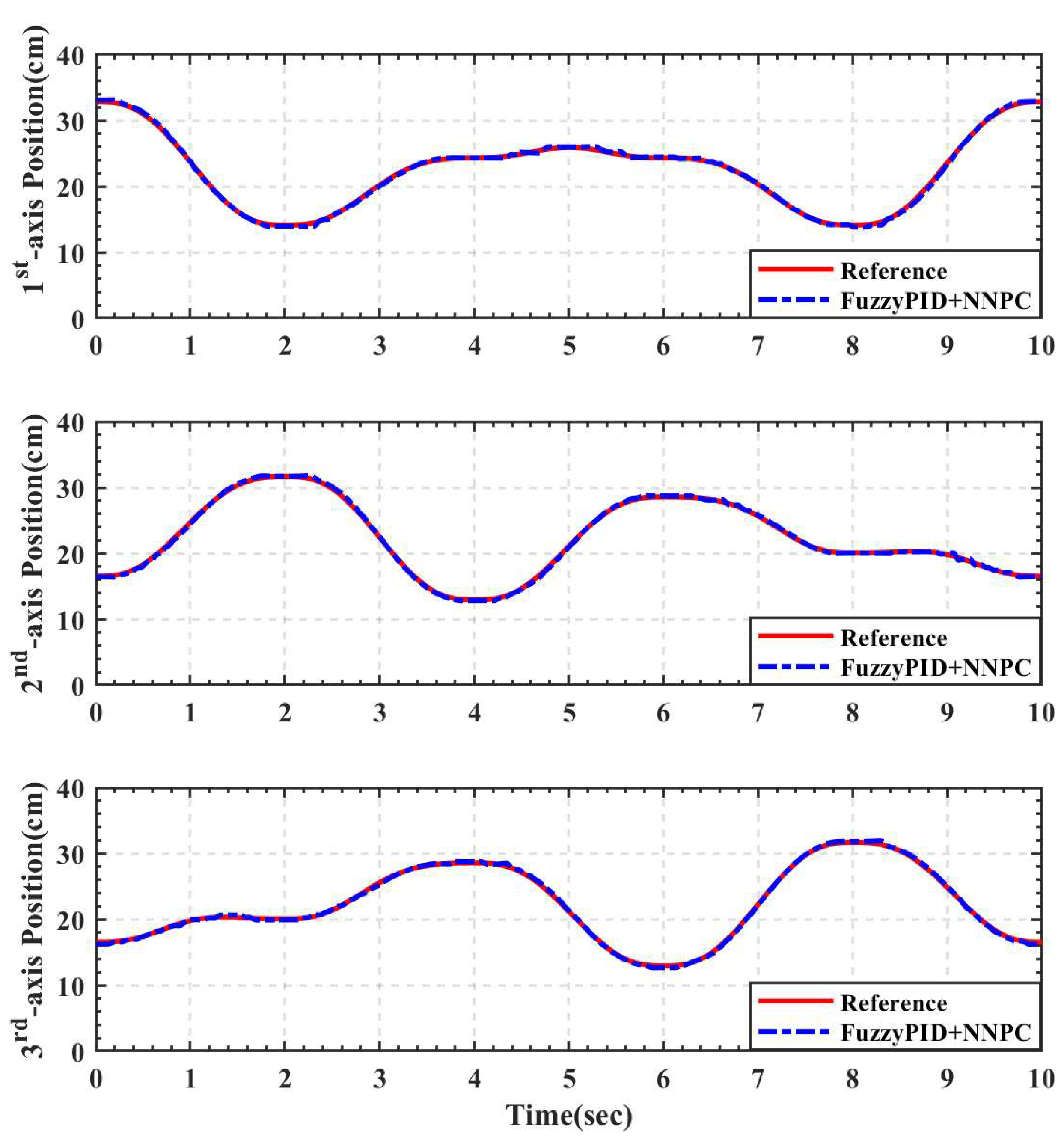
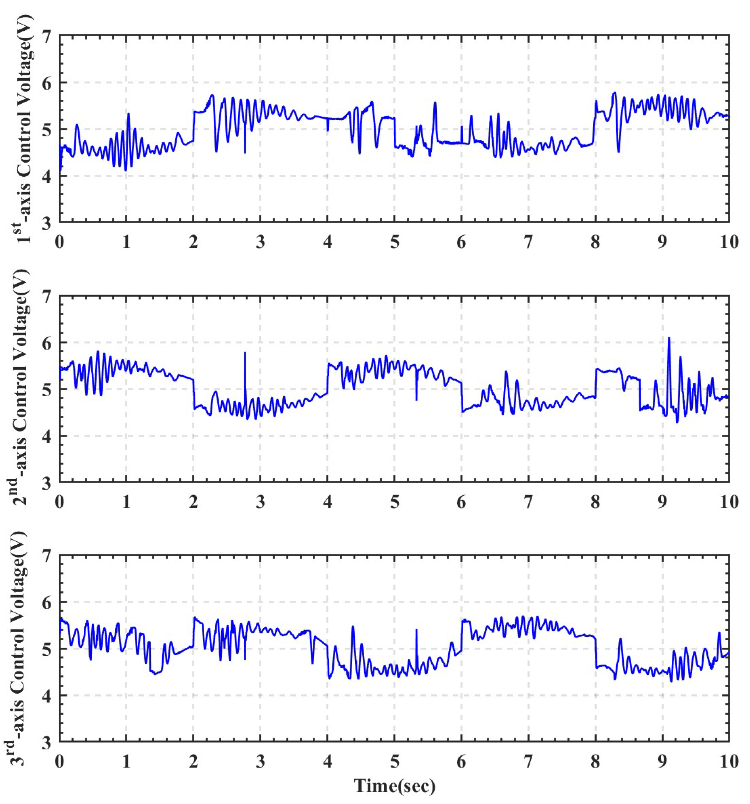
Figure 10 shows the desired star loop motion trajectory and the movement of the moving platform and the overall error . Figure 11 shows the desired trajectories and the system responses for the three rod-less PAs. Figure 12 shows the control voltages of the proportional servo valve for the 1st-axis, the 2nd-axis, and the 3rd-axis rod-less PA when the end-effector moves along the star loop motion trajectory. The proportional servo valve can adjust a spool according to input-voltage to change compressed air that flows into the chambers of a rod-less PA. Initially, the input-voltage is set to 5 V to remain the piston at the center of the rod-less PA in the experiments. Figure 13 shows the tracking errors of the 1st-axis, the 2nd-axis and the 3rd-axis rod-less PAs. The tracking error for the 1st-axis is within ±0.6 cm; the tracking error for the 2nd-axis is within ±0.58 cm; the tracking error for the 3rd-axis is within ±0.6 cm; and the maximum of for the star loop motion is less than 0.65 cm. There is a large tracking error in the start loop trajectory when the command position is suddenly changed; otherwise, the tracking error is very small. The results show good contour tracking for the star loop motion trajectory.
5.2. Experiment 2—Helical Circular Motion Trajectory
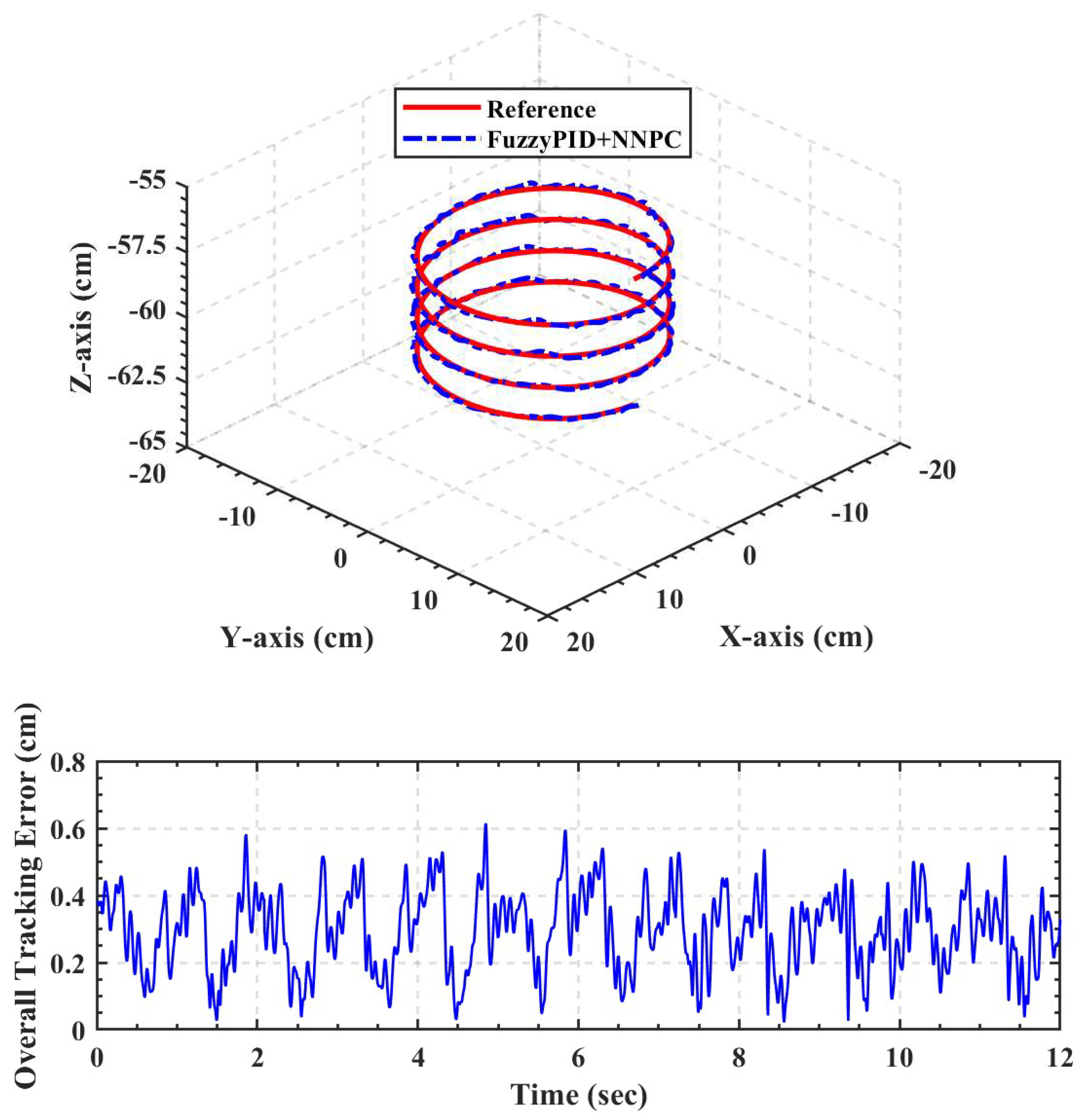
In Experiment 2, a helical circular motion trajectory is used to conduct space trajectory tracking control for the PH-LDR. The tracking objective is to force the moving platform along the helical circular motion trajectory. To prevent the slider and the shock from touching at the ends of the stroke of the 1st-axis, the 2nd-axis and the 3rd-axis rod-less PAs during trajectory tracking, the center position of the specified helical circular trajectory is shifted by a bias that is larger than the amplitude of the trajectory. The overall trajectory has two segments: a fifth-order path that takes the slider from the zero position to the starting point of the helical circular motion trajectory, and a segment wherein the platform moves along a helical circular motion trajectory. The helical circular motion trajectory is shown in Figure 14. The trajectory is formulated as [25]:
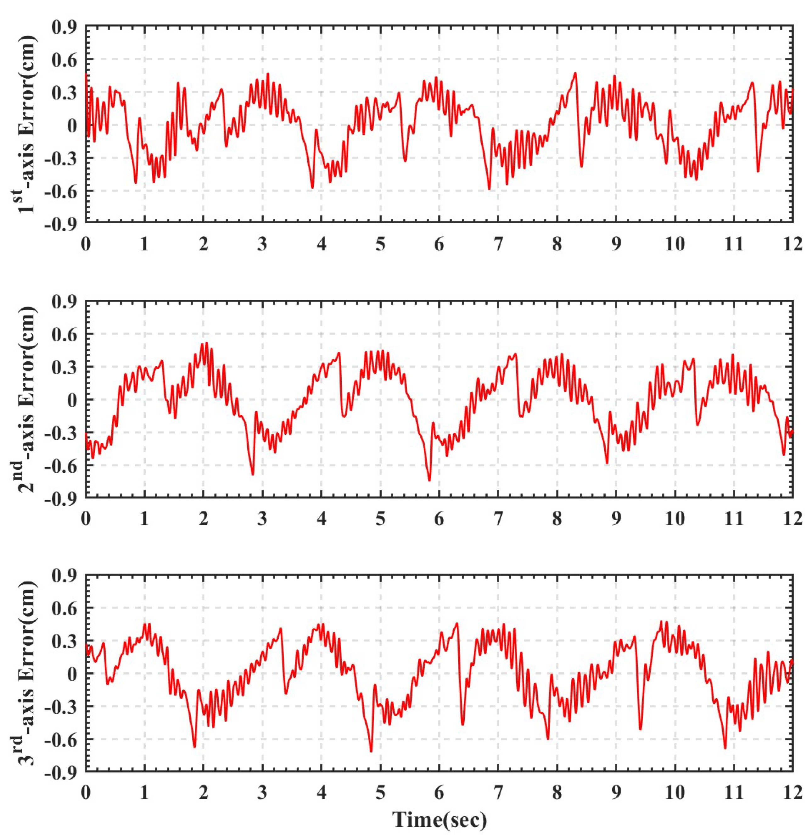
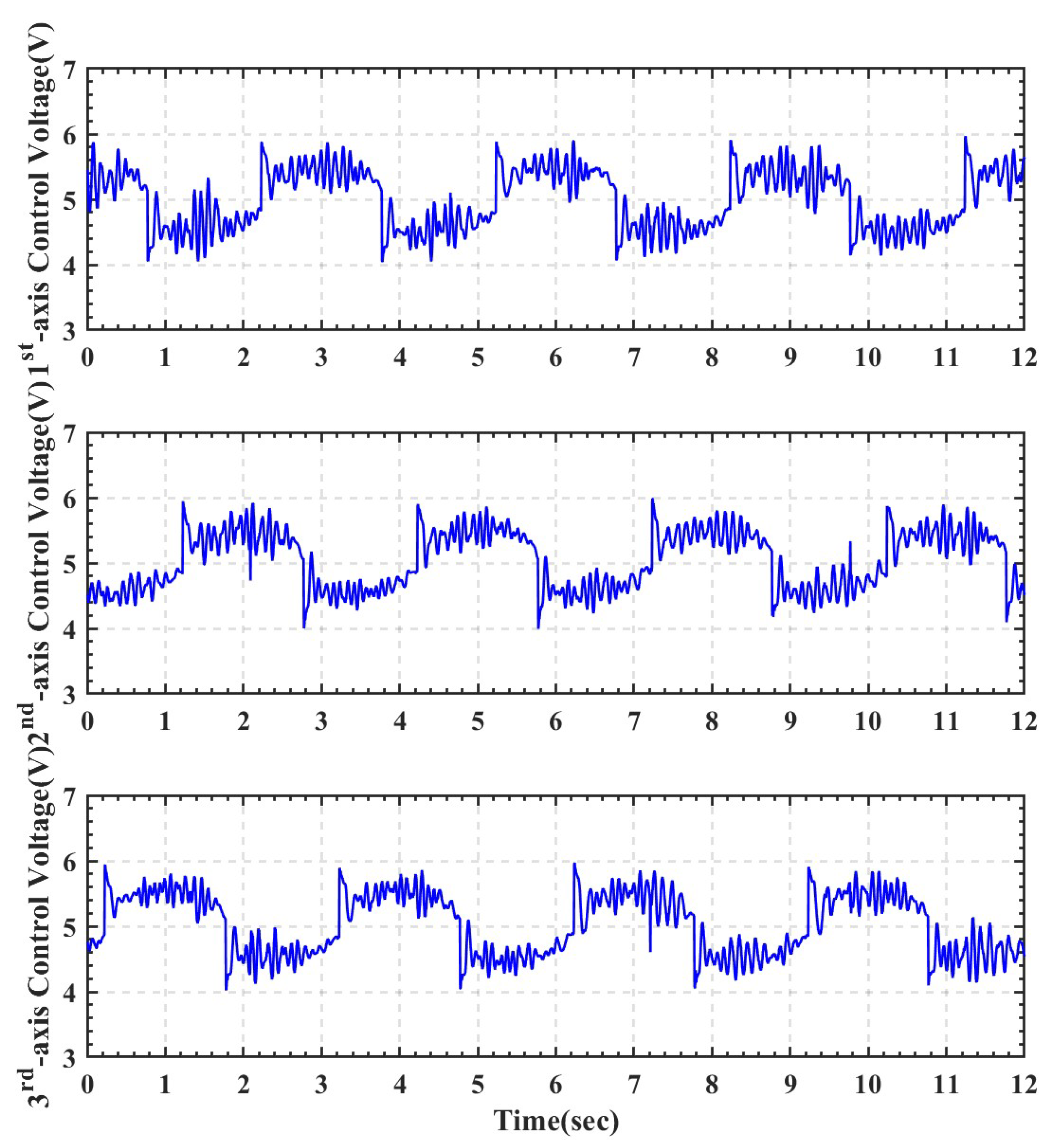
where , and are the increment of the angle, the increment of the z-axis, the radius, the x-axis position, the y-axis position, and the z-axis position of the moving platform, respectively. The helical circular tracking motion has a trajectory that is described by Equation (36), where the radius are within the interval of and are from −65 cm to −60 cm. The desired path and the system response for the moving platform for the helical circular trajectory are shown in Figure 15. The maximum of for the overall helical circular motion is less than 0.61 cm. Figure 16 shows the desired trajectories and the system responses for the three rod-less PAs. Figure 17 shows the control voltages of the proportional servo valve for the 1st-axis, the 2nd-axis, and the 3rd-axis rod-less PA when the end-effector moves along the star loop motion trajectory. The proportional servo valve can adjust a spool according to input-voltage to change compressed air that flows into the chambers of a rod-less PA. Initially, the input-voltage is set to 5 V to remain the piston at the center of the rod-less PA in the experiments. Figure 18 shows the tracking errors of the 1st-axis, 2nd-axis and 3rd-axis for the rod-less PAs when the platform moves along the helical circular trajectory, where the tracking error for the 1st-axis is within ±0.6 cm, the tracking error for the 2nd-axis is within ±0.7 cm, and the tracking error for the 3rd-axis is within ±0.7 cm. The tracking error in the 3-DOF motion contour tracking for the overall helical circular motion is small. Figure 15, Figure 16, Figure 17 and Figure 18 show that the proposed rod-less PAs based PH-LDR is effective and accurate.
6. Conclusions
This study develops a PH-LDR that consists of three rod-less PAs in a horizontal structure, so that a larger workspace can be yielded for the end-effector of LDR to achieve 3-DOF trajectory tracking. The parallel mechanism of the PH-LDR is analyzed based on a geometric method to determine the closed-form solutions of the kinematic chains. Moreover, a full-scale test-rig is experimentally set up in order to verify the feasibility of the proposed PH-LDR. For realizing the trajectory tracking control, a hybrid controller consisting of fuzzy-PID controller and NNPC is proposed, to overcome the nonlinearities and uncertainties resulted from the air compressibility and temperature change in the motion control of the pneumatic actuating system. From the experimental results, the design and construction of the PH-LDR system is verified through complex 3-DOF motion tracking control, including a star loop trajectory and a helical circular trajectory, on the developed test rig. In addition, the proposed architecture of LDR with the control methodologies can also be easily extended to the other 3D parallel mechanism robot, with modification of the workspace and the drive system.
7. Patents
This section is not mandatory, but may be added if there are patents resulting from the work reported in this manuscript.
Author Contributions
Conceptualization, L.-W.L. and H.-H.C.; methodology, L.-W.L. and I.-H.L.; software, H.-H.C. and I.-H.L.; validation, L.-W.L., H.-H.C. and I.-H.L.; formal analysis, L.-W.L. and H.-H.C.; investigation, L.-W.L. and H.-H.C.; resources, L.-W.L.; data curation, L.-W.L. and H.-H.C.; Writing—Original draft preparation, L.-W.L.; Writing—Review and editing, H.-H.C. and I.-H.L.; supervision, I.-H.L. and L.-W.L.; project administration, L.-W.L.; funding acquisition, L.-W.L. All authors have read and agreed to the published version of the manuscript.
Funding
This research has two financial support streams; from (1) Ministry of Science and Technology, R. O. C. Grant: (MOST 108-2628-E-005-003-MY2); (2) TBI MOTION Technology CORP., LTD.
Acknowledgments
This research is sponsored by the Ministry of Science and Technology, Taiwan, R.O.C., under Grants No. MOST 108-2628-E-005-003-MY2 and MOST 108-2221-E-032-047-.
Conflicts of Interest
The authors declare no conflict of interest.
References
- Li, Y.; Shang, D.; Fan, X.; Liu, Y. Motion reliability analysis of the delta parallel robot considering mechanism errors. Math. Probl. Eng. 2019. [Google Scholar] [CrossRef]
- Arockia, S.A.; Arul, K.M. Experimental investigation on position analysis of 3—DOF parallel manipulators. Procedia Eng. 2014, 97, 1126–1134. [Google Scholar]
- Patel, Y.D.; George, P.M. Parallel manipulators applications—A survey. Mod. Mech. Eng. 2012, 2, 57–64. [Google Scholar] [CrossRef] [Green Version]
- Ben-Dov, E.; Salcudean, S.E. A force-controlled pneumatic actuator. IEEE Trans. Robot. Autom. 1995, 11, 906–911. [Google Scholar] [CrossRef]
- Richer, E.; Hurmuzlu, Y. A high performance pneumatic force actuator system: Part II—Nonlinear controller design. J. Dyn. Syst. Meas. Control 1999, 122, 426–434. [Google Scholar] [CrossRef]
- Wang, J.; Wang, D.; Moore, P.R.; Pu, J. Modelling study, analysis and robust servocontrol of pneumatic cylinder actuator systems. IEE Proc. Control Theory Appl. 2001, 148, 35–42. [Google Scholar] [CrossRef]
- Milutinovic, D.; Slavkovic, N.; Kokotovic, B.M.; Zivanovic, S.; Dimic, Z. Kinematic modeling of reconfigurable parallel robots based on delta concept. J. Prod. Eng. 2013, 15, 71–74. [Google Scholar]
- Choi, H.S.; Han, C.S.; Lee, K.Y.; Lee, S.H. Development of hybrid robot for construction works with pneumatic actuator. Autom. Constr. 2005, 14, 452–459. [Google Scholar] [CrossRef]
- Chiang, M.H.; Lin, H.T. Development of a 3D parallel mechanism robot arm with three vertical-axial pneumatic actuators combined with a stereo vision system. Sensors 2011, 11, 11476–11494. [Google Scholar] [CrossRef] [Green Version]
- Chiang, M.H.; Chen, Y.H.; Chou, W.H. Analysis and control of a three-axial pyramidal pneumatic parallel manipulator. In Proceedings of the 9th JFPS International Symposium on Fluid Power, Matsue, Japan, 28–31 October 2014. [Google Scholar]
- Boudjedir, C.E.; Boukhetala, D.; Bouri, M. Nonlinear PD plus sliding mode control with application to a parallel delta robot. J. Electr. Eng. 2018, 69, 329–336. [Google Scholar] [CrossRef] [Green Version]
- Andrzej, L.P.; Emanuel, T.J.; Slawomir, B. Design of a 3-DOF tripod electro-pneumatic parallel manipulator. Robot. Auton. Syst. 2015, 72, 59–70. [Google Scholar]
- Lafmejani, A.S.; Masouleh, M.T.; Kalhor, A. Trajectory tracking control of a pneumatically actuated 6-DOF Gough–Stewart parallel robot using backstepping-sliding mode controller. Robot. Comput. Integr. Manuf. 2018, 54, 96–114. [Google Scholar] [CrossRef]
- Yan, S.J.; Ong, S.K.; Nee, A.Y.C. Optimization design of general triglide parallel manipulators. Adv. Robot. 2016, 30, 1027–1038. [Google Scholar] [CrossRef]
- Dongton, X.; Sun, Z. Kinematic reliability and sensitivity analysis of the modified delta parallel mechanism. Mach. Des. Manuf. 2016, 10, 167–169. [Google Scholar]
- Fu, J.; Gao, F.; Chen, W.; Pan, Y.; Lin, R. Kinematic accuracy research of a novel six-degree-of-freedom parallel robot with three legs. Mech. Mach. Theory 2016, 102, 86–102. [Google Scholar] [CrossRef]
- Liu, S.; Bobrow, J.E. An analysis of a pneumatic servo system and its application to a computer-controlled robot. J. Dyn. Syst. Meas. Control 1988, 110, 228–235. [Google Scholar] [CrossRef]
- Bone, G.M.; Shu, N. Experimental comparison of position tracking control algorithms for pneumatic cylinder actuators. IEEE ASME Trans. Mechatron. 2007, 12, 557–561. [Google Scholar] [CrossRef]
- Lee, L.W.; Li, I.H. Wavelet-based adaptive sliding-mode control with tracking performance for pneumatic servo system position tracking control. IET Control Theory Appl. 2012, 6, 1–16. [Google Scholar] [CrossRef]
- Lee, L.W.; Li, I.H. Design and implementation of a robust FNN-based adaptive sliding-mode controller for pneumatic actuator systems. J. Mech. Sci. Technol. 2016, 30, 381–396. [Google Scholar] [CrossRef]
- Tsai, L.W. Robot Analysis: The Mechanics of Serial and Parallel Manipulators; Wiley-Interscience: Hoboken, NJ, USA, 1999. [Google Scholar]
- Waldron, K.J.; Hunt, K.H. Series-parallel dualities in actively coordinated mechanisms. Int. J. Robot. Res. 1991, 10, 473–480. [Google Scholar] [CrossRef]
- Jankowski, K. Inverse Dynamics Control in Robotics Applications; Trafford Publishing: Bloomington, IN, USA, 2004. [Google Scholar]
- Hou, Y.; Zhao, Y. Workspace analysis and optimization of 3-PUU parallel mechanism in medicine base on genetic algorithm. Open Biomed. Eng. J. 2015, 9, 214–218. [Google Scholar] [CrossRef] [PubMed] [Green Version]
- Kung, Y.S.; Lin, J.M.; Chen, Y.J.; Chou, H.H. Model sim/simulink cosimulation and FPGA realization of a multiaxis motion controller. Math. Probl. Eng. 2015, 2015, 1–17. [Google Scholar] [CrossRef] [Green Version]
Figure 1.
Test-rig layout for the pneumatic-driven and horizontal-structure linear delta robot (PH-LDR).
Figure 1.
Test-rig layout for the pneumatic-driven and horizontal-structure linear delta robot (PH-LDR).

Figure 2.
Operation at the initial position for the rod-less pneumatic actuators (Pas).
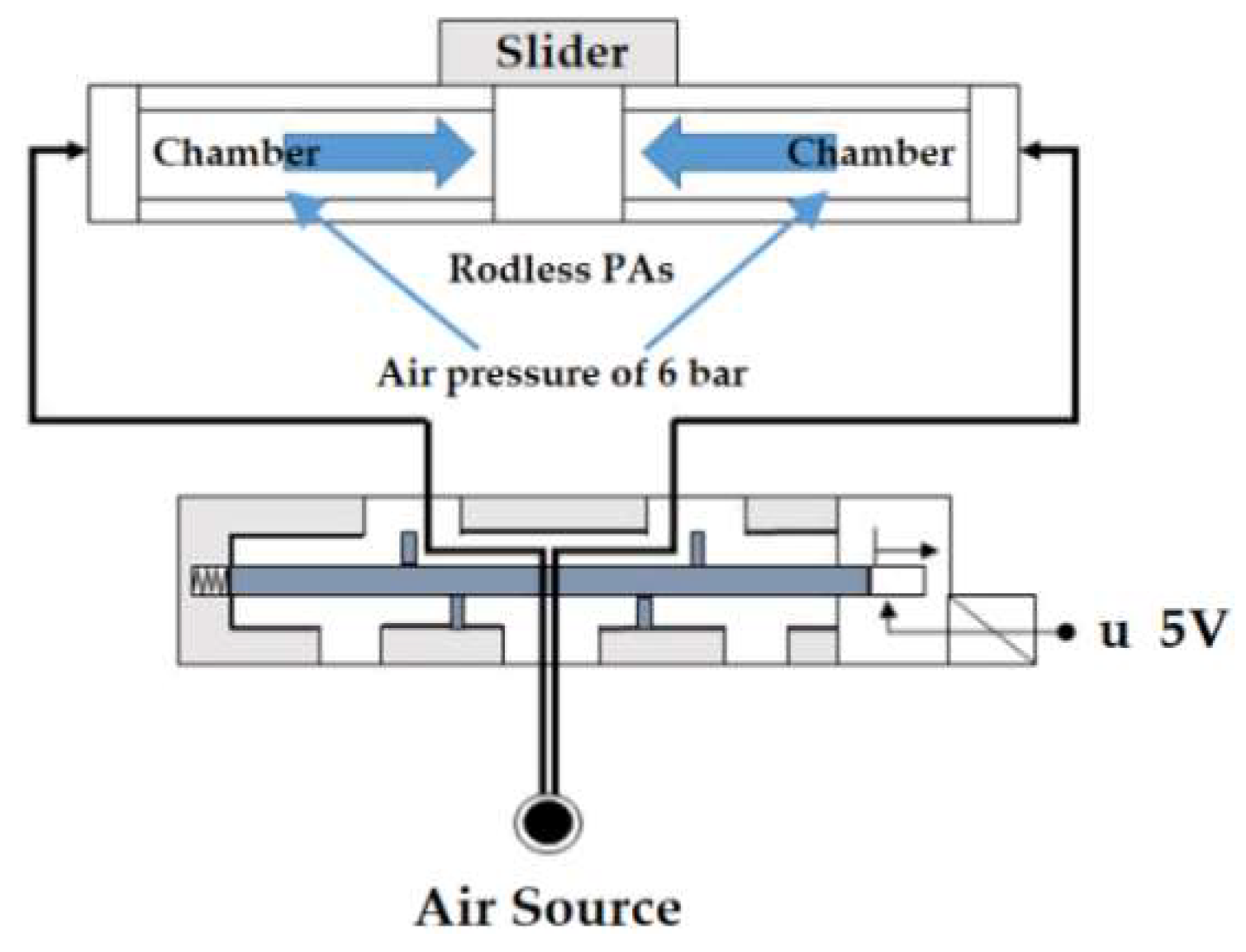
Figure 3.
Coordinate frames of the PH-LDR.
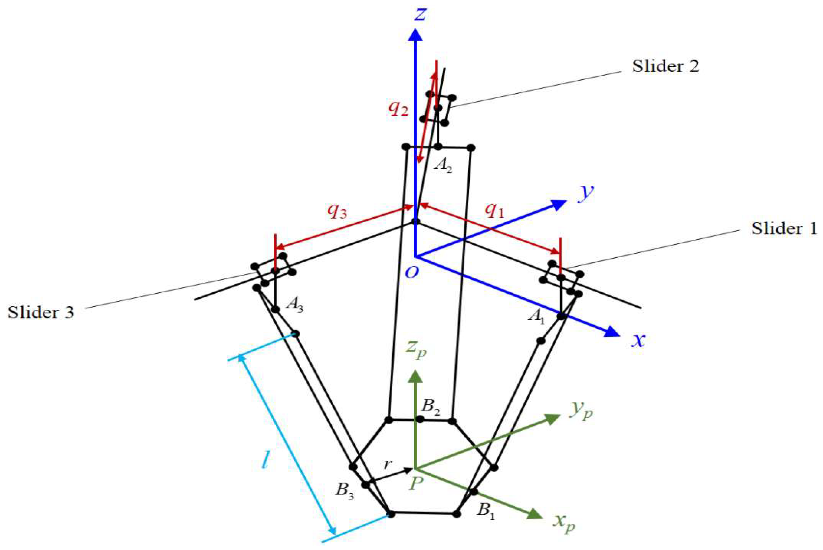
Figure 4.
Overall control system for the PH-LDR.
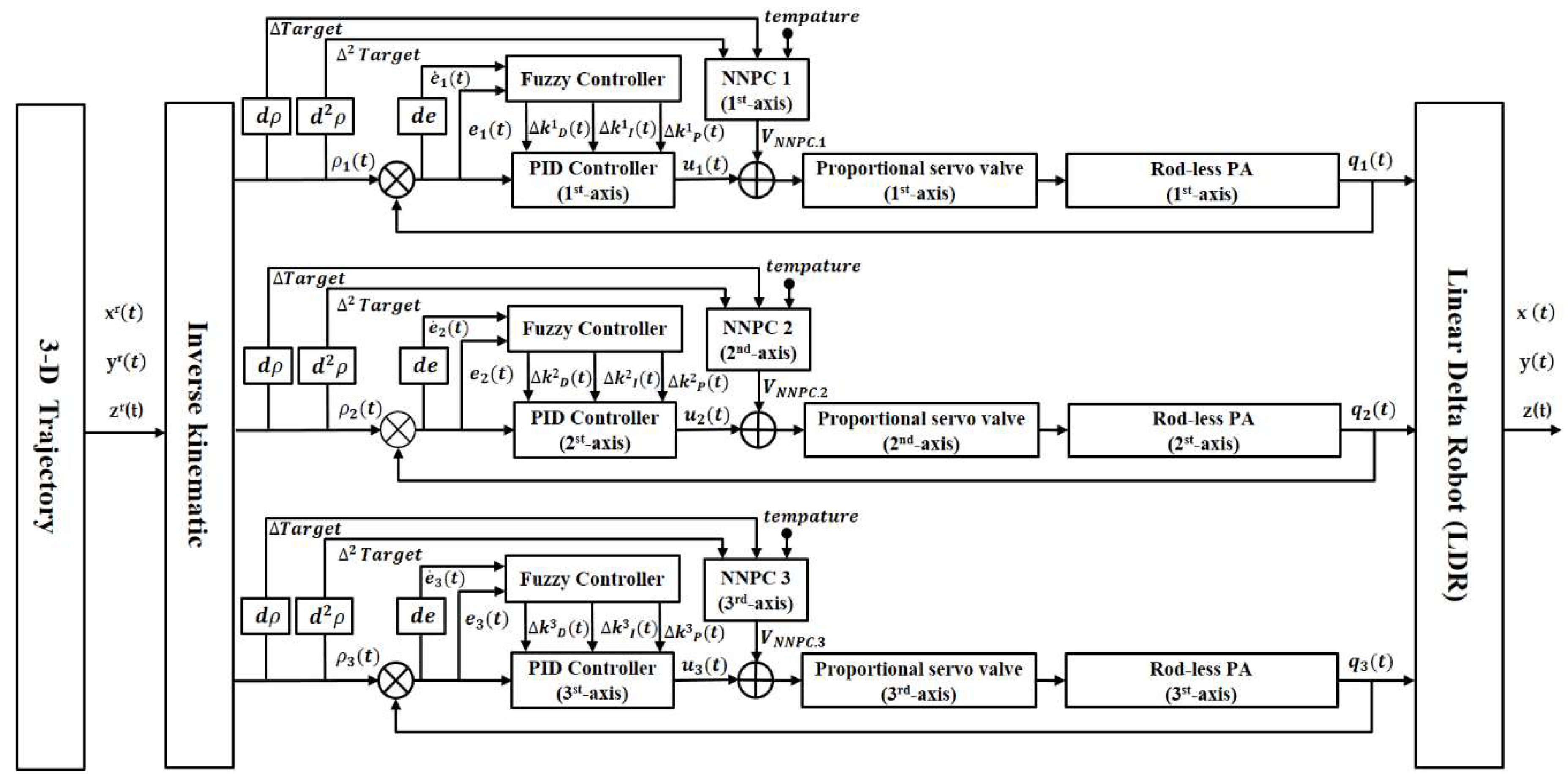
Figure 5.
Membership functions for (a) and (b) (c) and .

Figure 6.
Network Structure of the proposed NNPC.
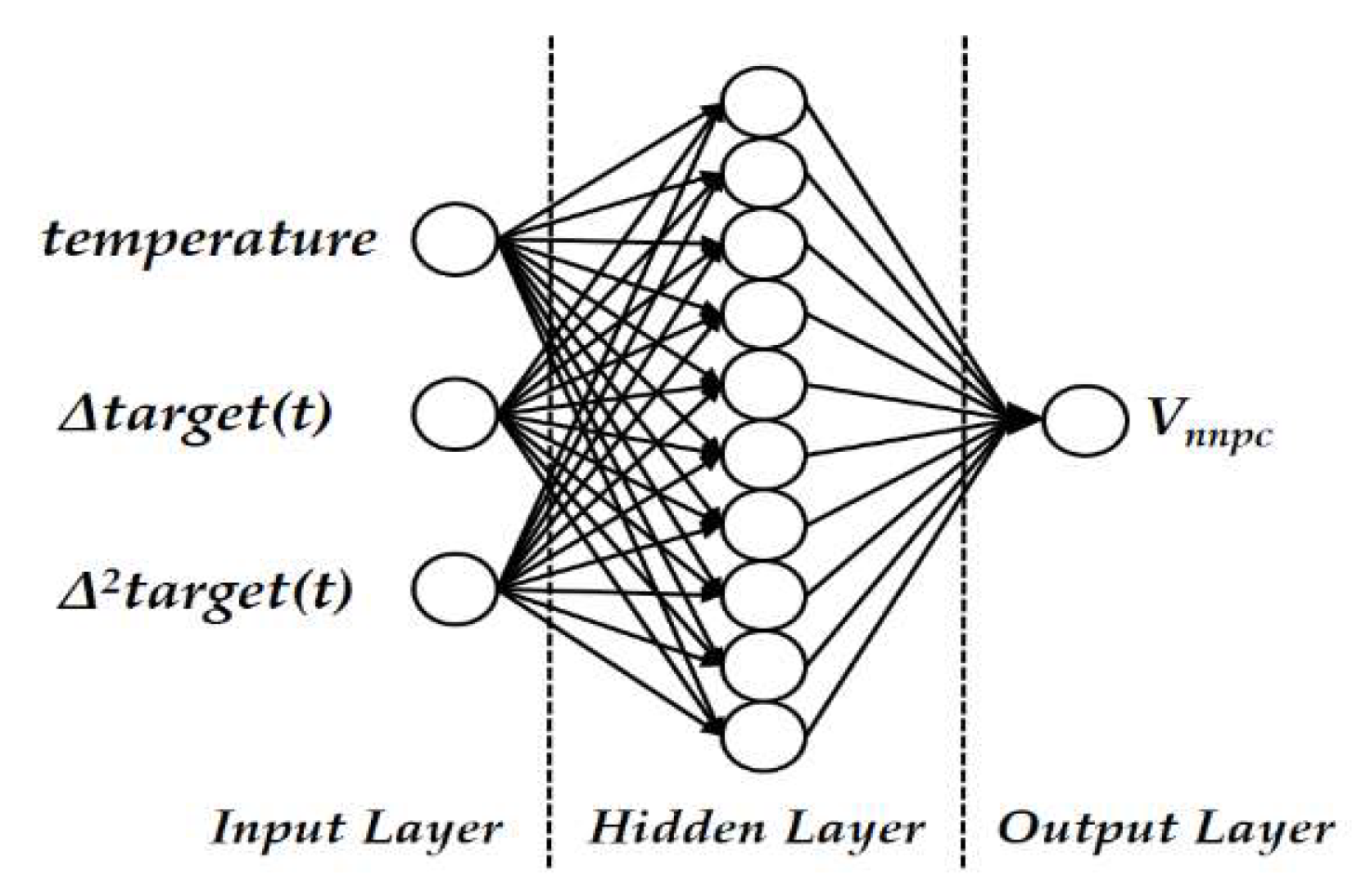
Figure 7.
The test-rig of PH-LDR.
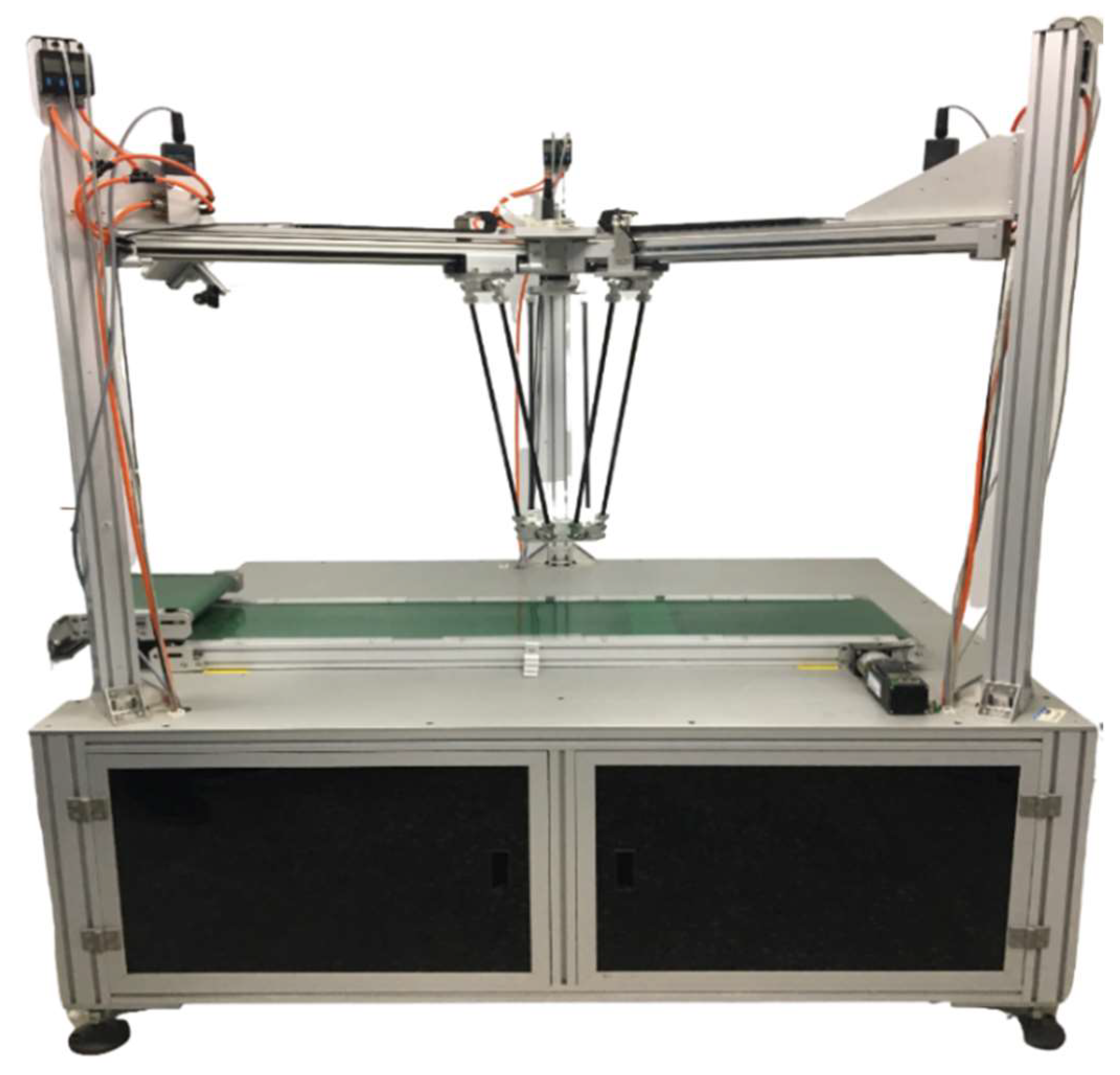
Figure 8.
Workspace of the PH-LDR using Monte Carlo method.
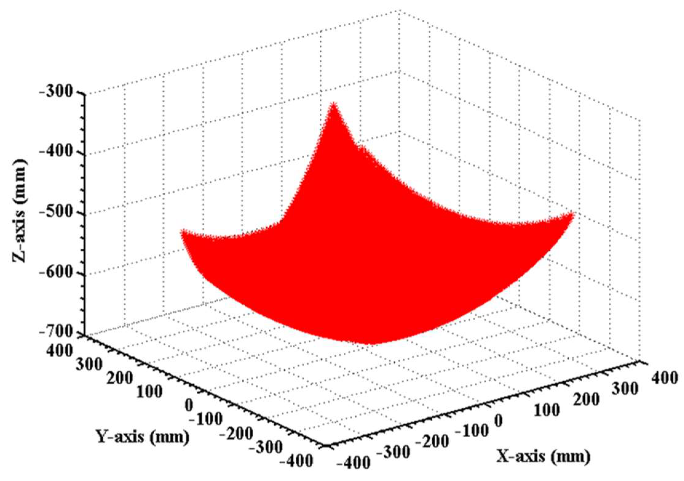
Figure 9.
The star loop trajectory.

Figure 10.
Star trajectory tracking and the overall error, as defined in Equation (34).
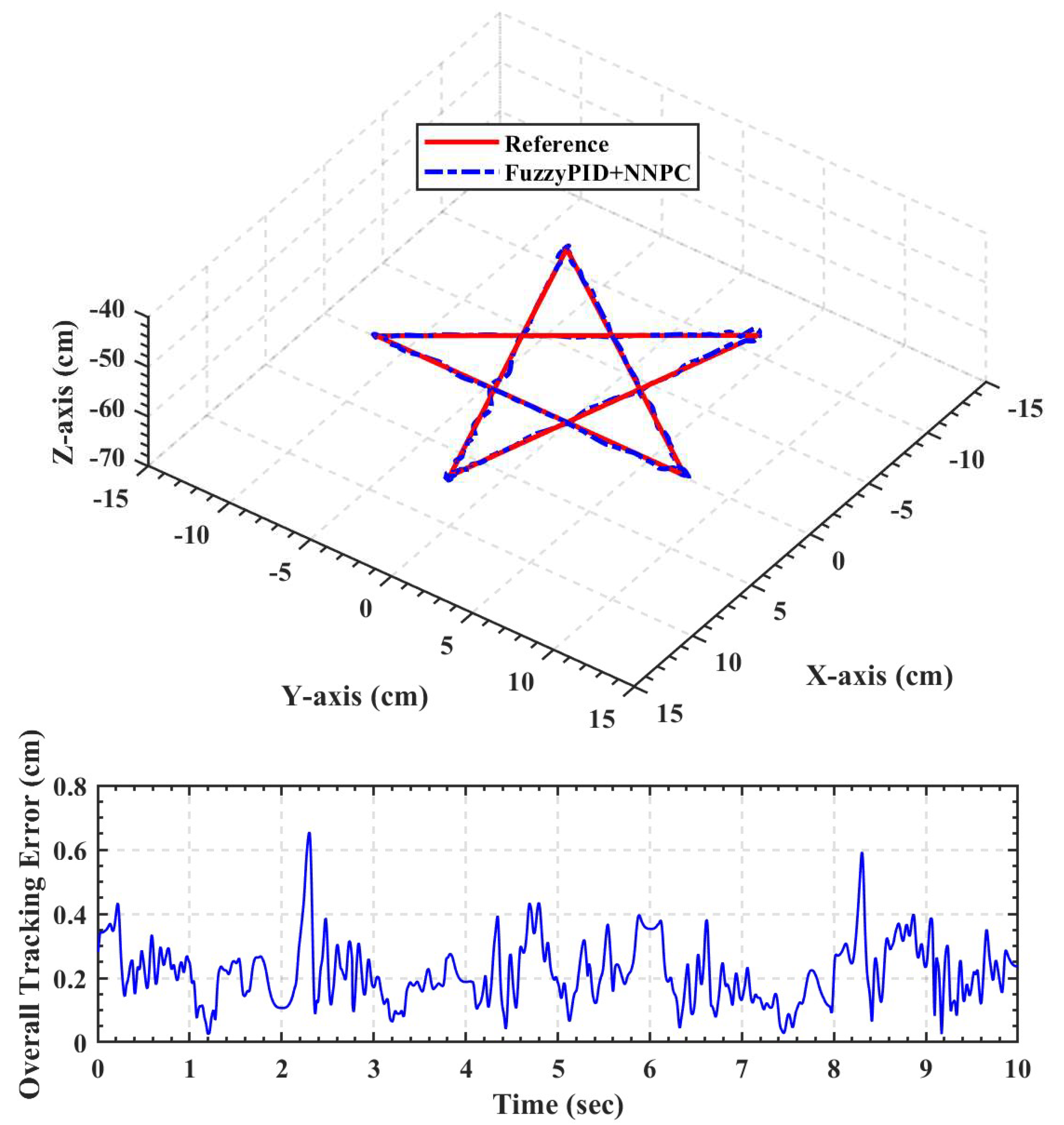
Figure 11.
Position tracking for the star trajectory for the 1st-axis, the 2nd-axis and the 3rd-axis rod-less PAs.
Figure 11.
Position tracking for the star trajectory for the 1st-axis, the 2nd-axis and the 3rd-axis rod-less PAs.

Figure 12.
Control voltages for the star trajectory for the 1st-axis, the 2nd-axis and the 3rd-axis rod-less PAs.
Figure 12.
Control voltages for the star trajectory for the 1st-axis, the 2nd-axis and the 3rd-axis rod-less PAs.

Figure 13.
Tracking errors for the star trajectory for the 1st-axis, the 2nd-axis and the 3rd-axiss rod-less PAs.
Figure 13.
Tracking errors for the star trajectory for the 1st-axis, the 2nd-axis and the 3rd-axiss rod-less PAs.
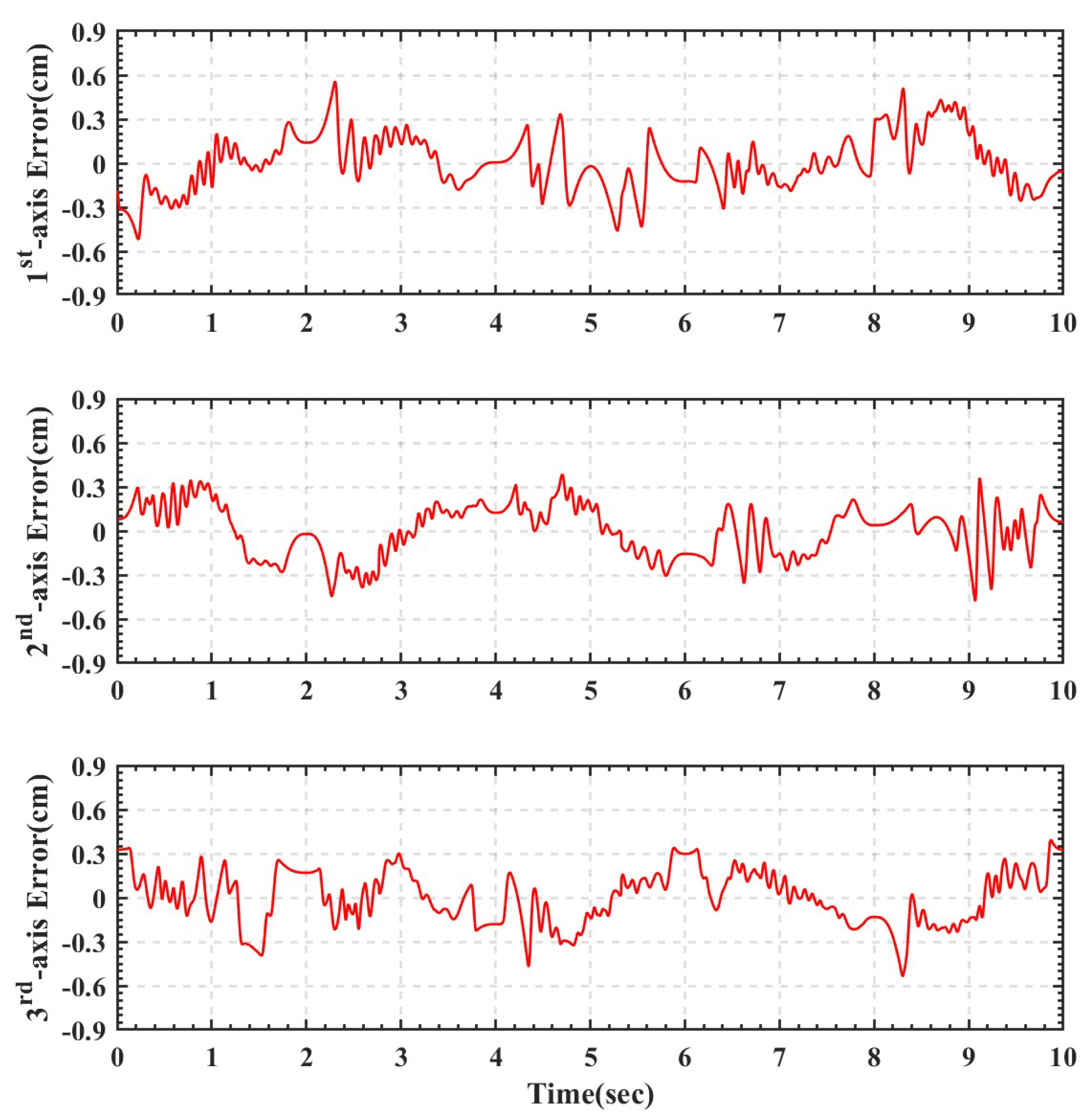
Figure 14.
Helical circular trajectory.
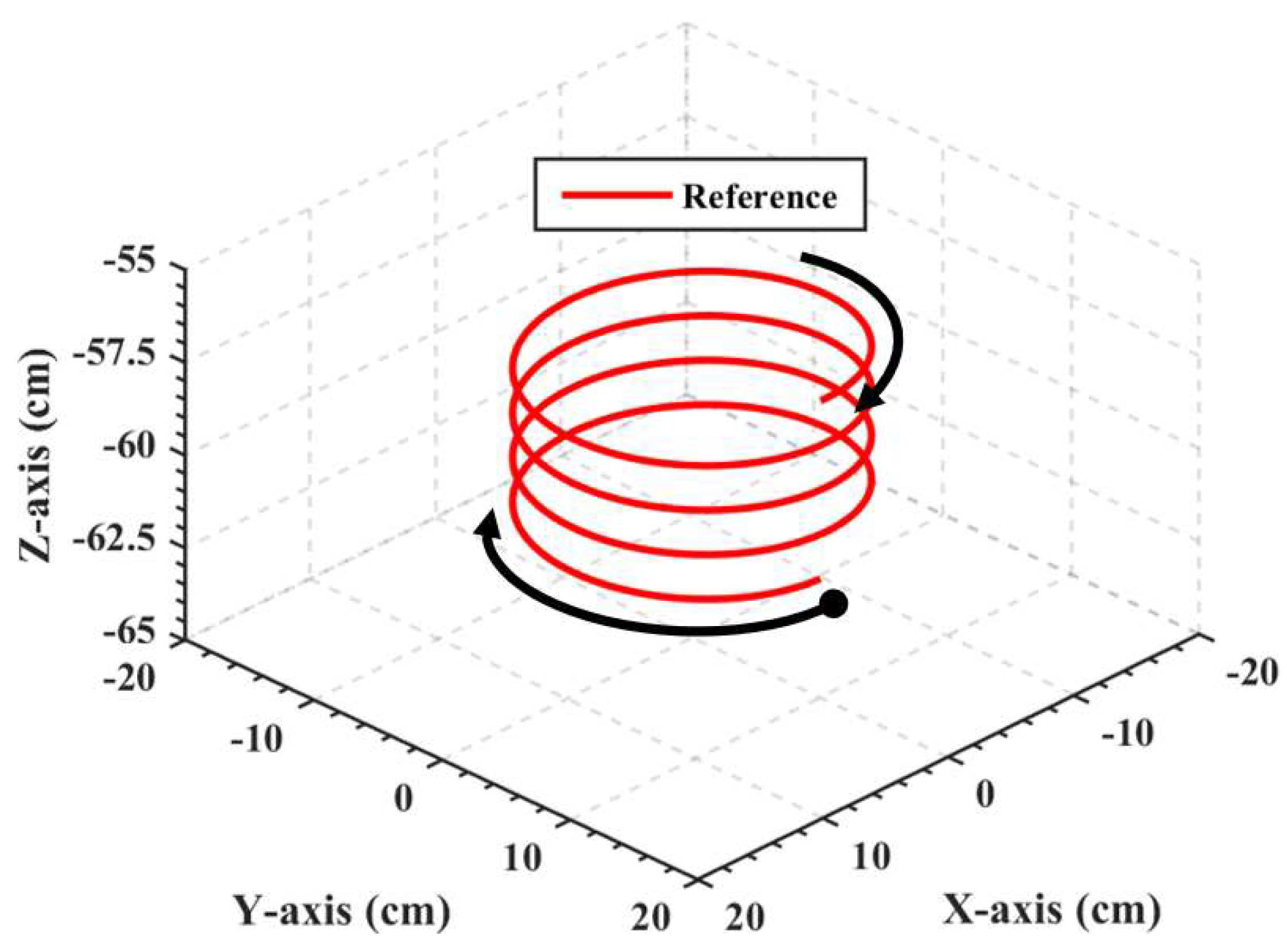
Figure 15.
Helical circular trajectory tracking and the overall error, as defined in Equation (34).

Figure 16.
Position tracking for the helical circular trajectory for the 1st-axis, the 2nd-axis and the 3rd-axis rod-less PAs.
Figure 16.
Position tracking for the helical circular trajectory for the 1st-axis, the 2nd-axis and the 3rd-axis rod-less PAs.
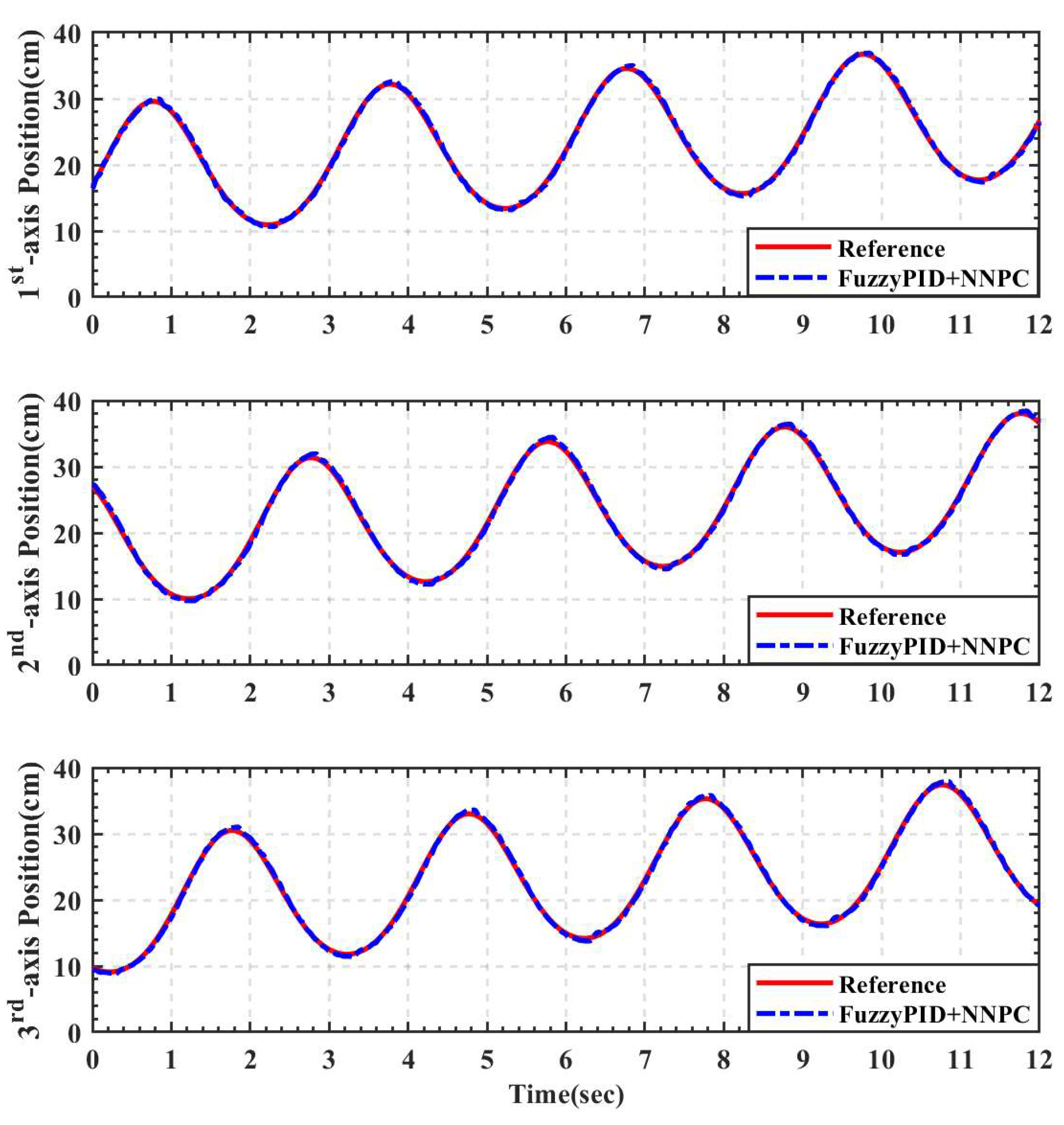
Figure 17.
Control voltages for the helical circular for the 1st-axis, the 2nd-axis and the 3rd-axis rod-less PAs.
Figure 17.
Control voltages for the helical circular for the 1st-axis, the 2nd-axis and the 3rd-axis rod-less PAs.

Figure 18.
Tracking errors for the helical circular trajectory for the 1st-axis, the 2nd-axis and the 3rd-axis rod-less PAs.
Figure 18.
Tracking errors for the helical circular trajectory for the 1st-axis, the 2nd-axis and the 3rd-axis rod-less PAs.

Table 1.
Geometry parameters for the PH-LDR.
| Parameters | Description | Value |
|---|---|---|
| The length between and | 60 mm | |
| The length of kinematic chain | 670 mm | |
| The maximum of the actuated joint variables (the maximum stroke) | 500 mm |
Table 2.
The fuzzy rules for .
| NB | NM | NS | ZO | PS | PM | PB | ||
|---|---|---|---|---|---|---|---|---|
| NB | PB | PB | PM | PM | PS | ZO | ZO | |
| NM | PB | PB | PM | PS | PS | ZO | NS | |
| NS | PM | PM | PM | PS | ZO | NS | NS | |
| ZO | PM | PM | PS | ZO | NS | NM | NM | |
| PS | PS | PS | ZO | NS | NS | NM | NM | |
| PM | PS | ZO | NS | NM | NM | NM | NB | |
| PB | ZO | ZO | NM | NM | NM | NB | NB | |
Table 3.
The fuzzy rules for .
| NB | NM | NS | ZO | PS | PM | PB | ||
|---|---|---|---|---|---|---|---|---|
| NB | NB | NB | NM | NM | NS | ZO | ZO | |
| NM | NB | NB | NM | NS | NS | ZO | ZO | |
| NS | NB | NM | NS | NS | ZO | PS | PS | |
| ZO | NM | NM | NS | ZO | PS | PM | PM | |
| PS | NM | NS | ZO | NS | PS | PM | PB | |
| PM | ZO | ZO | PS | PS | PM | PB | PB | |
| PB | ZO | ZO | PS | PM | PM | PB | PB | |
Table 4.
The fuzzy rules for .
| NB | NM | NS | ZO | PS | PM | PB | ||
|---|---|---|---|---|---|---|---|---|
| NB | PS | NS | NB | NB | NB | NB | PS | |
| NM | PS | NS | NB | NM | NM | NS | ZO | |
| NS | ZO | NS | NM | NM | NS | NS | ZO | |
| ZO | ZO | NS | NS | NS | NS | NS | ZO | |
| PS | ZO | ZO | ZO | ZO | ZO | ZO | ZO | |
| PM | PB | NS | PS | PS | PS | PS | PB | |
| PB | PB | PM | PM | PM | PS | PS | PB | |
© 2020 by the authors. Licensee MDPI, Basel, Switzerland. This article is an open access article distributed under the terms and conditions of the Creative Commons Attribution (CC BY) license (http://creativecommons.org/licenses/by/4.0/).
Share and Cite
MDPI and ACS Style
Li, I.-H.; Chiang, H.-H.; Lee, L.-W. Development of A Linear Delta Robot with Three Horizontal-Axial Pneumatic Actuators for 3-DOF Trajectory Tracking. Appl. Sci. 2020, 10, 3526. https://doi.org/10.3390/app10103526
AMA Style
Li I-H, Chiang H-H, Lee L-W. Development of A Linear Delta Robot with Three Horizontal-Axial Pneumatic Actuators for 3-DOF Trajectory Tracking. Applied Sciences. 2020; 10(10):3526. https://doi.org/10.3390/app10103526
Chicago/Turabian StyleLi, I-Hsum, Hsin-Han Chiang, and Lian-Wang Lee. 2020. "Development of A Linear Delta Robot with Three Horizontal-Axial Pneumatic Actuators for 3-DOF Trajectory Tracking" Applied Sciences 10, no. 10: 3526. https://doi.org/10.3390/app10103526
Note that from the first issue of 2016, this journal uses article numbers instead of page numbers. See further details here.