Computation of Stray Losses in Transformer Bushing Regions Considering Harmonics in the Load Current


 ,
,
Abstract
1. Introduction
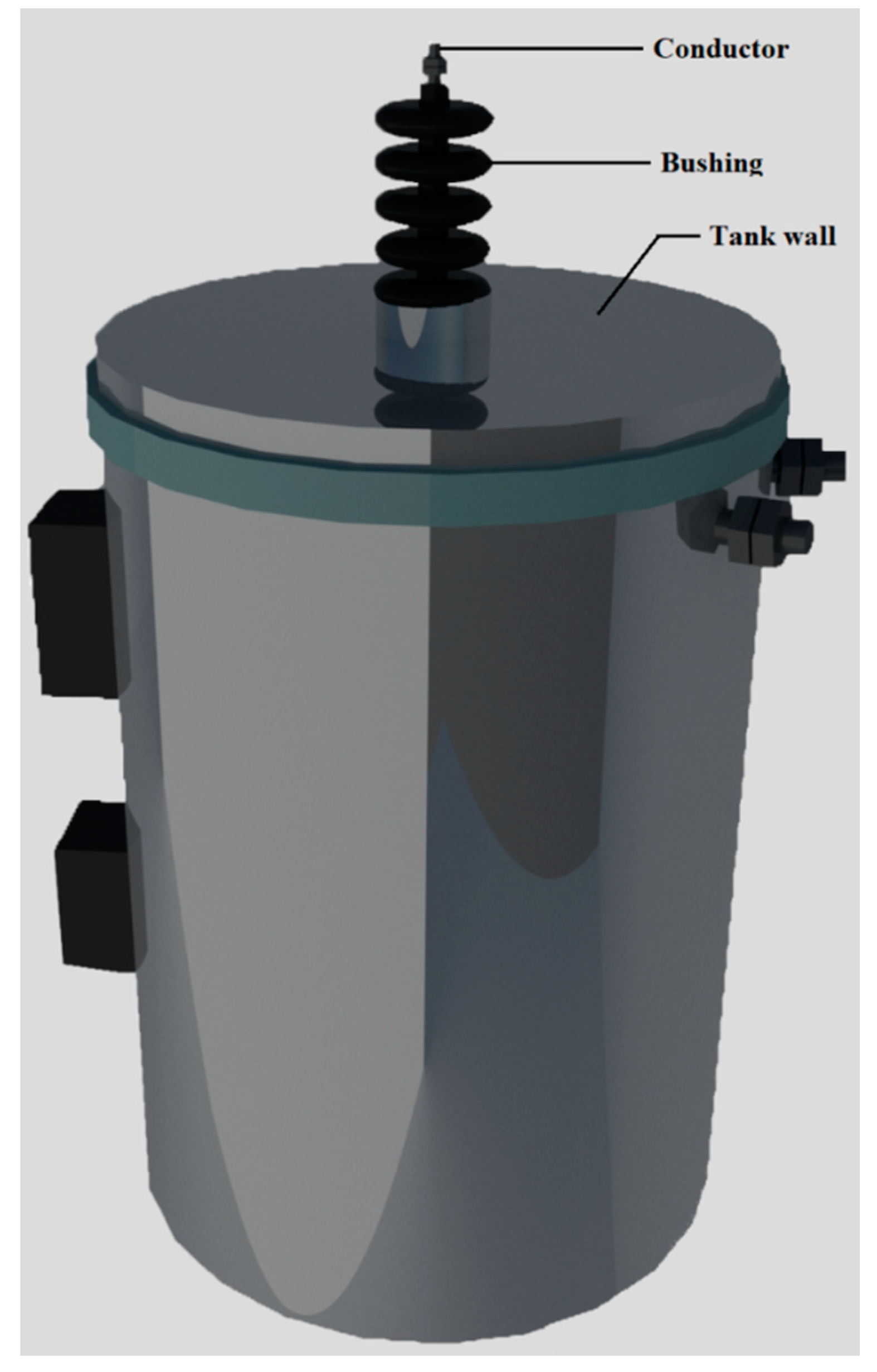
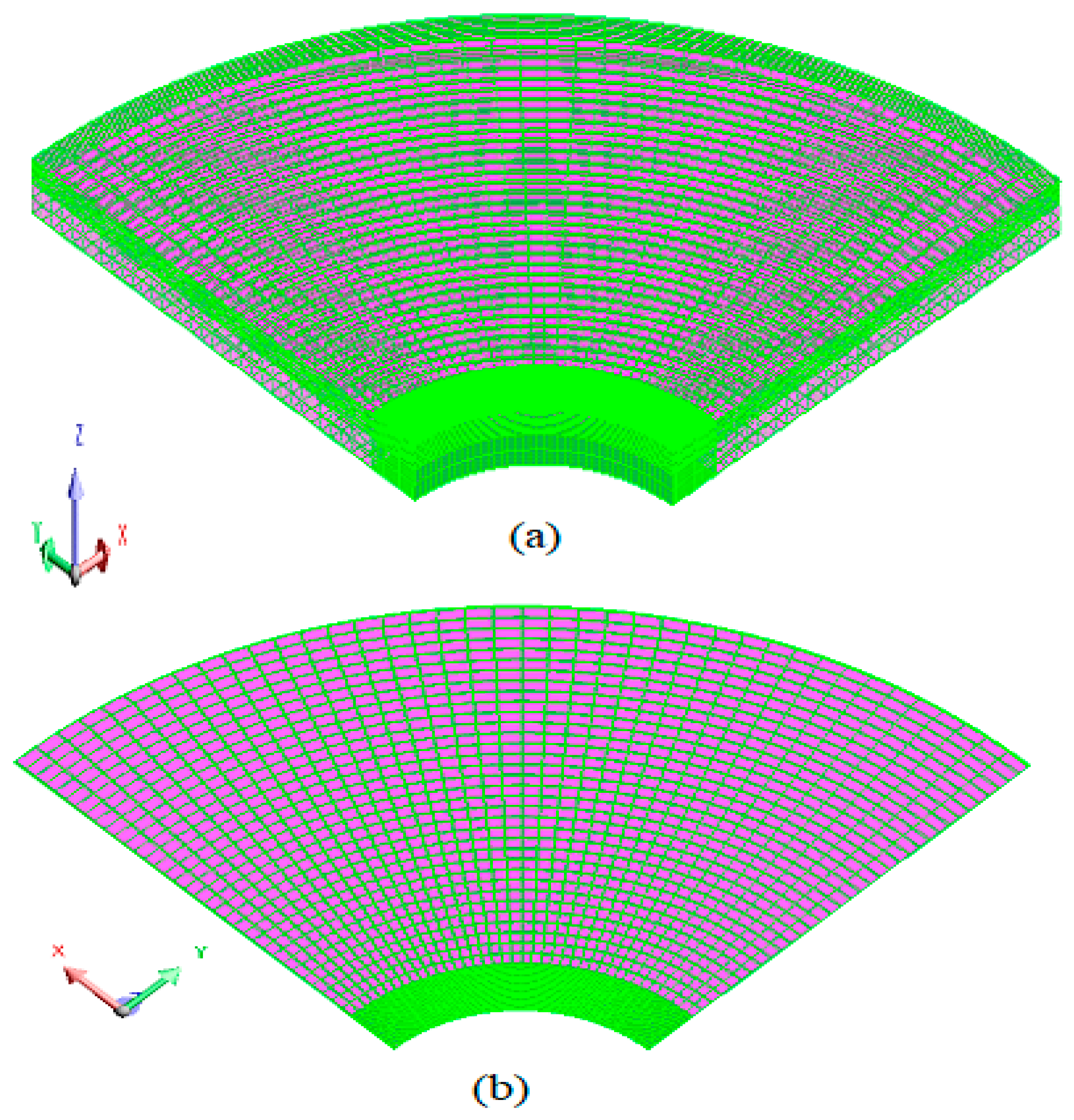
2. Model
3. Electromagnetic Field (EMF) Distribution in Region
4. Coupling of Solutions in Regions and
5. Electric Field (EF) and Eddy Current (EC) Losses in the Tank Wall
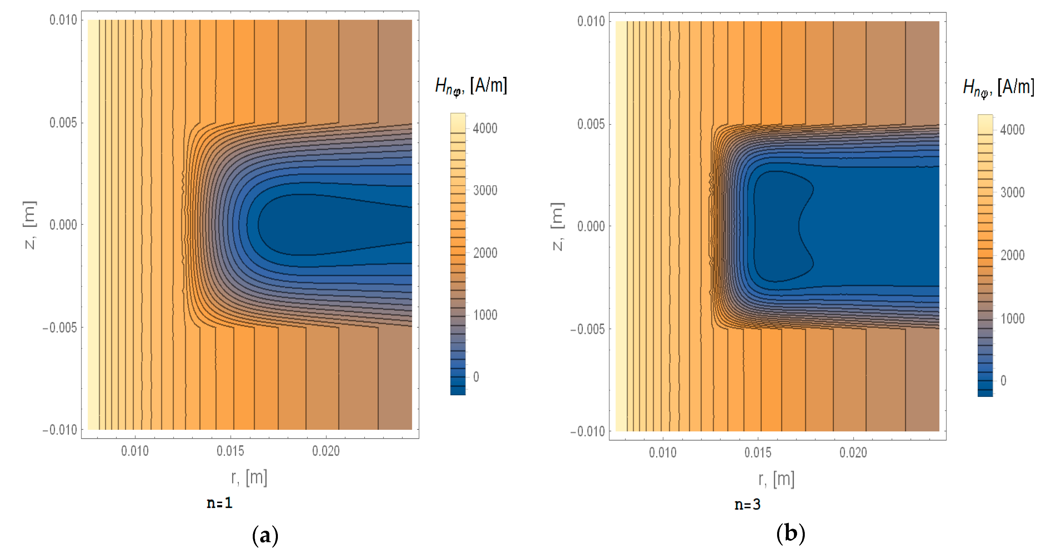
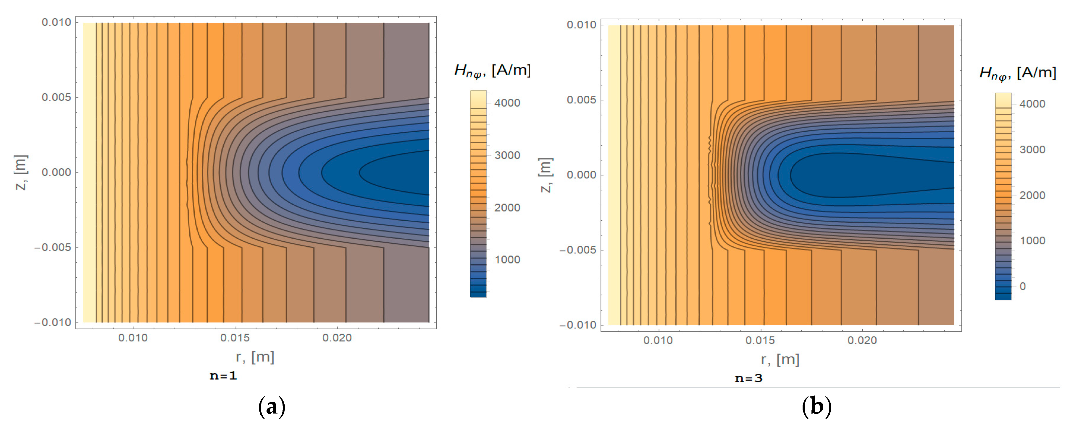
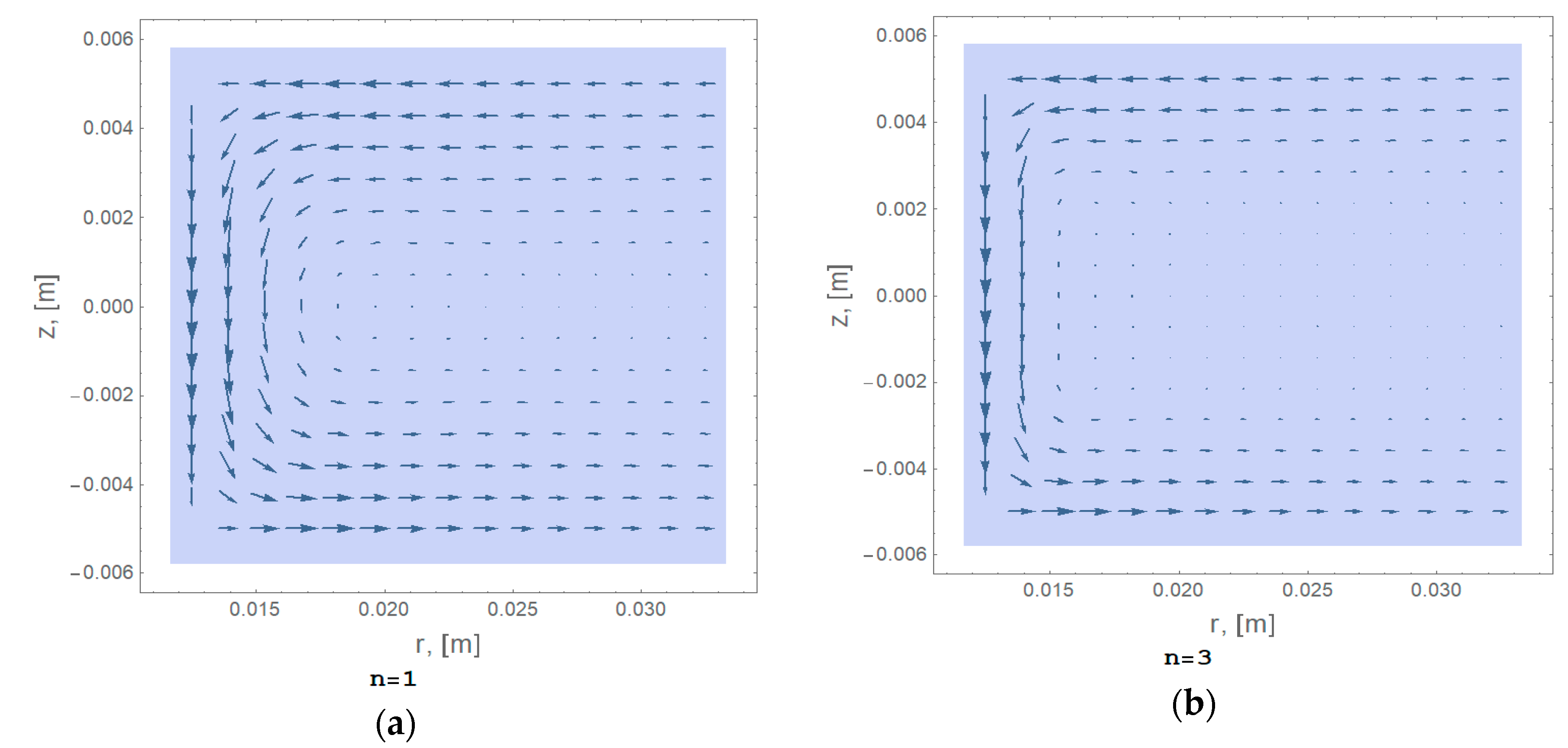
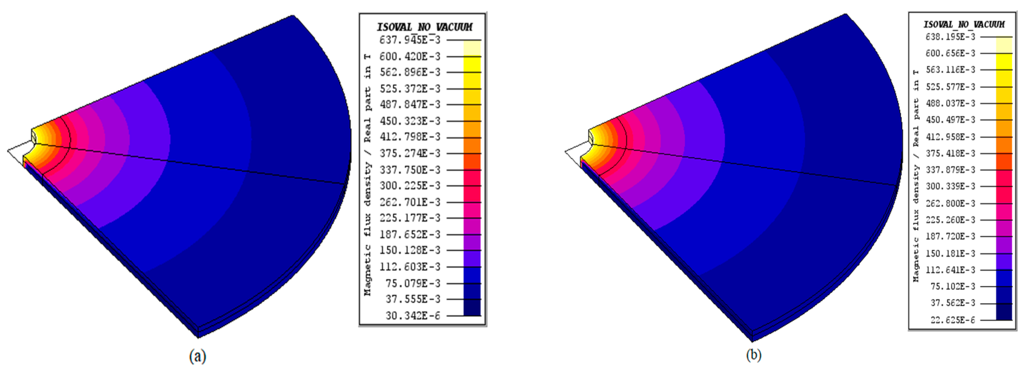
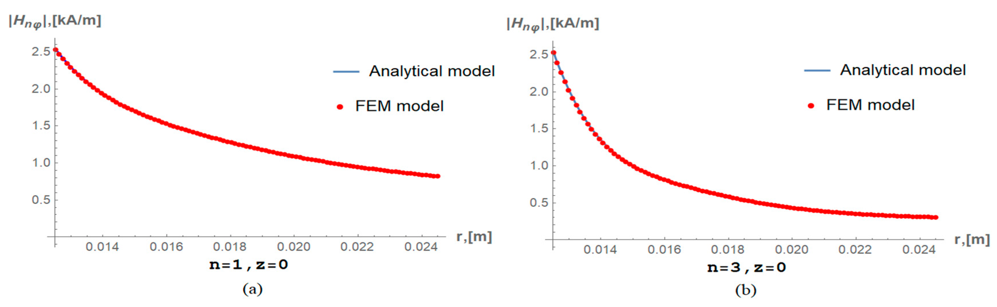
6. Simulation Results and Discussion
7. Conclusions
Author Contributions
Funding
Conflicts of Interest
References
- Kong, X.; Quan, S.; Sun, F.; Chen, Z.; Wang, X.; Zhou, Z. Two-Stage Optimal Scheduling of Large-Scale Renewable Energy System Considering the Uncertainty of Generation and Load. Appl. Sci. 2020, 10, 971. [Google Scholar] [CrossRef]
- Karimi, M.; Mokhlis, H.; Naidu, K.; Uddin, S.; Bakar, A.H.A. Photovoltaic penetration issues and impacts in distribution network A review. Renew. Sustain. Energy Rev. 2016, 53, 594–605. [Google Scholar] [CrossRef]
- Song, S.; Yoon, M.; Jang, G. Analysis of six active power control strategies of interconnected grids with VSC-HVDC. Appl. Sci. 2019, 9, 183. [Google Scholar] [CrossRef]
- Arranz-Gimon, A.; Zorita-Lamadrid, A.; Morinigo-Sotelo, D.; Duque-Perez, O. A Study of the Effects of Time Aggregation and Overlapping within the Framework of IEC Standards for the Measurement of Harmonics and Interharmonics. Appl. Sci. 2019, 9, 4549. [Google Scholar] [CrossRef]
- Petrović, P.; Damljanović, N. New procedure for harmonics estimation based on Hilbert transformation. Electr. Eng. 2017, 99, 313. [Google Scholar] [CrossRef]
- Kalair, A.; Abas, N.; Kalair, A.R.; Saleem, Z.; Khan, N. Review of harmonic analysis, modeling and mitigation techniques. Renew. Sustain. Energy Rev. 2017, 78, 1152–1187. [Google Scholar]
- Faiz, J.; Ghazizadeh, M.; Oraee, H. Derating of transformers under non-linear load current and non-sinusoidal voltage an overview. IET Electr. Power Appl. 2015, 9, 486–495. [Google Scholar] [CrossRef]
- Faiz, J.; Ebrahimi, B.M.; Ghofrani, M. Mixed Derating of Distribution Transformers Under Unbalanced Supply Voltage and Nonlinear Load Conditions Using TSFEM. IEEE Trans. Power Deliv. 2010, 25, 780–789. [Google Scholar] [CrossRef]
- Christina, A.J.; Salam, M.A.; Rahman, Q.M.; Wen, F.; Ang, S.P.; Voon, W. Causes of transformer failures and diagnostic methods–A review. Renew. Sustain. Energy Rev. 2018, 82, 1442–1456. [Google Scholar]
- Metwally, I.A. Failures, Monitoring and New Trends of Power Transformers. IEEE Potentials 2011, 30, 36–43. [Google Scholar] [CrossRef]
- Ho, S.L.; Li, Y.; Wong, H.C.; Wang, S.H.; Tang, R.Y. Numerical simulation of transient force and eddy current loss in a 720-MVA power transformer. IEEE Trans. Magn. 2004, 40, 687–690. [Google Scholar] [CrossRef]
- Di Pasquale, A.; Antonini, G.; Orlandi, A. Shielding effectiveness for a three-phase transformer at various harmonic frequencies. IET Sci. Meas. Technol. 2009, 3, 175–183. [Google Scholar] [CrossRef]
- Zia Zahedi, M.; Iskender, I. Nonlinear Adaptive Magneto-Thermal Analysis at Bushing Regions of a Transformers Cover Using Finite Difference Method. J. Therm. Sci. Eng. Appl. 2019, 11. [Google Scholar] [CrossRef]
- Lopez-Fernandez, X.M.; Penabad-Duran, P.; Turowski, J. Three-dimensional methodology for the overheating hazard assessment on transformer covers. IEEE Trans. Ind. Appl. 2012, 48, 1549–1555. [Google Scholar] [CrossRef]
- Turowski, J.; Pelikant, A. Eddy current losses and hot-spot evaluation in cover plates of power transformers. IEE Proc.-Electr. Power Appl. 1997, 144, 435–440. [Google Scholar] [CrossRef]
- Junyou, Y.; Renyuan, T.; Yan, L.; Yongbin, C. Eddy current fields and overheating problems due to heavy current carrying conductors. IEEE Trans. Magn. 1994, 30, 3064–3067. [Google Scholar] [CrossRef]
- Zahedi, M.Z.; Iskender, I. FDM electromagnetic analysis in bushing regions of transformer. Int. J. Tech. Phys. Prob. Eng. 2018, 10, 27–33. [Google Scholar]
- Penabad-Duran, P.; Lopez-Fernandez, X.M.; Turowski, J. 3D non-linear magneto-thermal behavior on transformer covers. Electr. Power Syst. Res. 2015, 121, 333–340. [Google Scholar] [CrossRef]
- Del Vecchio, R.M.; Poulin, B.; Feeney, M.E.F.; Feghali, P.T.; Shah, D.M.; Ahuja, R.; Shah, D.M. Transformer Design Principles: With Applications to Core-Form Power Transformers, 2nd ed.; CRC Press: Washington, DC, USA, 2001; pp. 412–418. [Google Scholar]
- Maximov, S.; Olivares-Galvan, J.C.; Magdaleno-Adame, S.; Escarela-Perez, R.; Campero-Littlewood, E. New analytical formulas for electromagnetic field and eddy current losses in bushing regions of transformers. IEEE Trans. Magn. 2015, 51, 1–10. [Google Scholar] [CrossRef]
- Saito, S.; Inagaki, K.; Sato, T.; Inui, Y.; Okuyama, K.; Otani, H. Eddy currents in structure surrounding large currents bushing of a large capacity transformer. IEEE Trans. Power App. Syst. 1981, 100, 4502–4509. [Google Scholar] [CrossRef]
- Renyuan, T.; Junyou, Y.; Feng, L.; Yongping, L. Solutions of three-dimensional Multiply Connected and Open Boundary Problems by BEM in Three-Phase Combinations Transformers. IEEE Trans. Magn. 1992, 28, 1340–1343. [Google Scholar] [CrossRef]
- Guerin, C.; Meunier, G.; Tanneau, G. Surface impedance for 3D nonlinear eddy current problems-application to loss computation in transformers. IEEE Trans. Magn. 1996, 32, 808–811. [Google Scholar] [CrossRef]
- Vladimirov, V.S. Equations of Mathematical Physics, Marcel Dekker, 1971: Equations of Mathematical Physics, 1st ed.; Marcel Dekker, Inc.: New York, NY, USA, 1971; pp. 263–269. [Google Scholar]
- Olver, F.W.J.; Lozier, D.M.; Boisvert, R.F.; Clark, C.W. NIST Handbook of Mathematical Functions; Cambridge University Press: New York, NY, USA, 2010; pp. 248–261. [Google Scholar]
- Olver, F.W.J. Asymptotics and Special Functions, 1st ed.; Academic Press: New York, NY, USA; London, UK, 1974; pp. 4–6. [Google Scholar]


| Case | A [m] | B [m] | h [m] | Irms [A] | Harmonic | |
|---|---|---|---|---|---|---|
| 1 | 0.0125 | 0.150 | 0.010 | 141.42 | n = 1 | |
| 2 | 0.0125 | 0.150 | 0.010 | 141.42 | n = 3 | |
| 3 | 0.04 | 0.145 | 0.00952 | 141.42 | n = 1 | |
| 4 | 0.04 | 0.145 | 0.00952 | 141.42 | n = 3 | |
| 5 | 0.04 | 0.145 | 0.00952 | 141.42 | n = 5 | |
| 6 | 0.035 | 0.140 | 0.00952 | 141.42 | n = 1 | |
| 7 | 0.035 | 0.140 | 0.00952 | 141.42 | n = 3 | |
| 8 | 0.035 | 0.140 | 0.00952 | 141.42 | n = 5 |
| Case | Ptotal [W], Analytical | Ptotal [W], Numerical | Relative Error (%) | Skin-Effect Depth, [mm] | Harmonic |
|---|---|---|---|---|---|
| 1 | 1.874 | 1.870 | 0.22 | 2.297 | n = 1 |
| 2 | 3.276 | 3.267 | 0.27 | 1.326 | n = 3 |
| 3 | 0.959 | 0.953 | 0.63 | 2.297 | n = 1 |
| 4 | 1.632 | 1.630 | 0.13 | 1.326 | n = 3 |
| 5 | 2.127 | 2.117 | 0.470 | 1.027 | n = 5 |
| 6 | 1.614 | 1.588 | 1.610 | 3.979 | n = 1 |
| 7 | 3.108 | 3.100 | 0.26 | 2.297 | n = 3 |
| 8 | 3.917 | 3.901 | 0.41 | 1.779 | n = 5 |
© 2020 by the authors. Licensee MDPI, Basel, Switzerland. This article is an open access article distributed under the terms and conditions of the Creative Commons Attribution (CC BY) license (http://creativecommons.org/licenses/by/4.0/).
Share and Cite
Khan, S.; Maximov, S.; Escarela-Perez, R.; Olivares-Galvan, J.C.; Melgoza-Vazquez, E.; Lopez-Garcia, I. Computation of Stray Losses in Transformer Bushing Regions Considering Harmonics in the Load Current. Appl. Sci. 2020, 10, 3527. https://doi.org/10.3390/app10103527
Khan S, Maximov S, Escarela-Perez R, Olivares-Galvan JC, Melgoza-Vazquez E, Lopez-Garcia I. Computation of Stray Losses in Transformer Bushing Regions Considering Harmonics in the Load Current. Applied Sciences. 2020; 10(10):3527. https://doi.org/10.3390/app10103527
Chicago/Turabian StyleKhan, Sohail, Serguei Maximov, Rafael Escarela-Perez, Juan Carlos Olivares-Galvan, Enrique Melgoza-Vazquez, and Irvin Lopez-Garcia. 2020. "Computation of Stray Losses in Transformer Bushing Regions Considering Harmonics in the Load Current" Applied Sciences 10, no. 10: 3527. https://doi.org/10.3390/app10103527
APA StyleKhan, S., Maximov, S., Escarela-Perez, R., Olivares-Galvan, J. C., Melgoza-Vazquez, E., & Lopez-Garcia, I. (2020). Computation of Stray Losses in Transformer Bushing Regions Considering Harmonics in the Load Current. Applied Sciences, 10(10), 3527. https://doi.org/10.3390/app10103527