Walsh Transform and Empirical Mode Decomposition Applied to Reconstruction of Velocity and Displacement from Seismic Acceleration Measurement

Abstract

This paper focuses on reconstruction of dynamic velocity and displacement from seismic acceleration signal. For conventional time-domain approaches or frequency-domain approaches, due to initial values and non-negligible noise in the acceleration signal, drift and deviation in velocity and displacement are inevitable. To deal with this deficiency, this paper develops a Walsh transform and Empirical Mode Decomposition (EMD)-based integral algorithm, or WATEBI in short. In the WATEBI algorithm, the Walsh transform is employed to realize vibration signal reconstruction. Next, the EMD method is used to eliminate the residual in the reconstructed signal. Finally, the trend term in velocity and displacement is removed by linear least-squares fit. This algorithm can be straightforwardly implemented by an ordinary computer. Reconstructed displacements and velocities from vibration of a simulated single-degree-of-freedom system and two-site measured ground motions in earthquakes validated the robustness and adaptiveness of this algorithm. It can be also applied to many other areas, like mechanical engineering and ocean engineering.

1. Introduction

With the rapid development of modern science and technology, the research on mechanical and structural vibration has promoted great advances in numerous engineering fields and areas, such as aerospace engineering, bridge engineering, earthquake engineering and offshore engineering [1,2]. In mechanical engineering, vibration tests have attracted considerable attention, as they are of significant value for the health monitoring of machinery [3], including system operational reliability and mechanical breakdown detection. In earthquake engineering, ground motion signals are the key to evaluating seismic magnitude and intensity [4]. Records of ground motions in a strong seismic event are an essential input to time-domain dynamic response calculation for structures located in earthquake-prone zones. Thus, it is important to obtain accurate vibration responses, either directly through in situ real-time monitoring, or indirectly through vibration tests and numerical reconstruction through data post-processing. Usually the responses of interest are acceleration, velocity, displacement, and stress signals of a structure. They can be measured by a wide variety of sensors. In most situations it is acceleration that is measured. Please note that the measured acceleration is an absolute quantity, while the measured displacement is relative to a reference object. In reality, it is not straightforward to install a fixed displacement sensor due to the geometrical complexity of a structure and its restricted ambient space [5]. By contrast, as a result of their small size, acceleration sensors need neither a large space nor a stationary reference [1]. Among concurrent motion sensors, acceleration sensors (for instance accelerometers) are technically the most versatile. It is very convenient in both laboratory tests and field observations to carry out acceleration logging.

To acquire data of unknown velocity and displacement, a traditional and popular approach is the integral of measured acceleration. There are two main integral schemes. One is by integrating the circuit and the other uses a numerical integral algorithm [6]. Circuit integration is rarely used as it is sensitive to the low frequency of acceleration, while the numerical integral scheme has been widely adopted for years. The numerical scheme can be divided into two categories, time-domain integral [5] and frequency-domain conversion [7]. The former includes known methods like trapezoid formula, Simpson’s rule, Newton-Cotes formula and first to Nth-order integral operator based on the Runge-Kutta algorithm. However, these conventional methods have several disadvantages [1]. The result usually exhibits drift and errors in the trend term [8] because of the contained direct current component, and high-frequency or low-frequency noise. The frequency-domain conversion method by contrast is numerically much faster, by transforming the time-domain acceleration into a curve synthesizing complex coefficients through finite Fourier series. Various Fast Fourier transform (FFT) algorithms have been widely applied to build the corresponding relationship between frequencies and amplitudes [9]. To solve the problem of spectral leakage in FFT, the antileakage least-squares spectral analysis (ALLSSA) [10] and multichannel ALLSSA [11] have been proposed to regularize the irregularly sampled series and to attenuate the random noise. They were proven more robust than the antileakage Fourier transform (ALFT) [12] and the arbitrarily sampled Fourier transform (ASFT) [13]. It follows that by the principle of trigonometric function integrals, the velocity and displacement signals in frequency domain could be obtained by simply dividing the Fourier coefficients of acceleration with transfer functions (iω) and (iω)². Then, the time series of velocity and displacement are recovered by applying the Inverse Fourier Transform (IFT) [7].

Many attempts have been proposed to improve the rationality and accuracy of the aforementioned methods. These attempts are categorized into three classes of integral approaches, the time-domain polynomial fitting to remove the trend error [14], the band-pass filtering method [15], and FFT implementation with low-frequency cutoff and attenuation attempts [16,17,18], have demonstrated their good applicability in engineering problems. Nevertheless, these approaches still have flaws with respect to error control and fidelity. Recent years have also seen the application of Hilbert-Huang transform and wavelet transform [19,20,21,22], such as the least-squares wavelet and cross-wavelet analyses [23]. However, these transforms have not yet been well established for signal conversion.

This paper proposes a Walsh Transform and Empirical Model Decomposition (EMD)-based Integral algorithm (WATEBI) to obtain the desired velocity and displacement from acceleration. To demonstrate the level of robustness and adaptiveness of this algorithm, three case studies are presented. The first study is a numerically simulated vibration of a single-degree-of-freedom (SDOF) system driven by white noise. The other two cases are seismic recordings including ground acceleration, velocity and displacement, respectively, measured in two typical earthquakes.

2. The Proposed Method

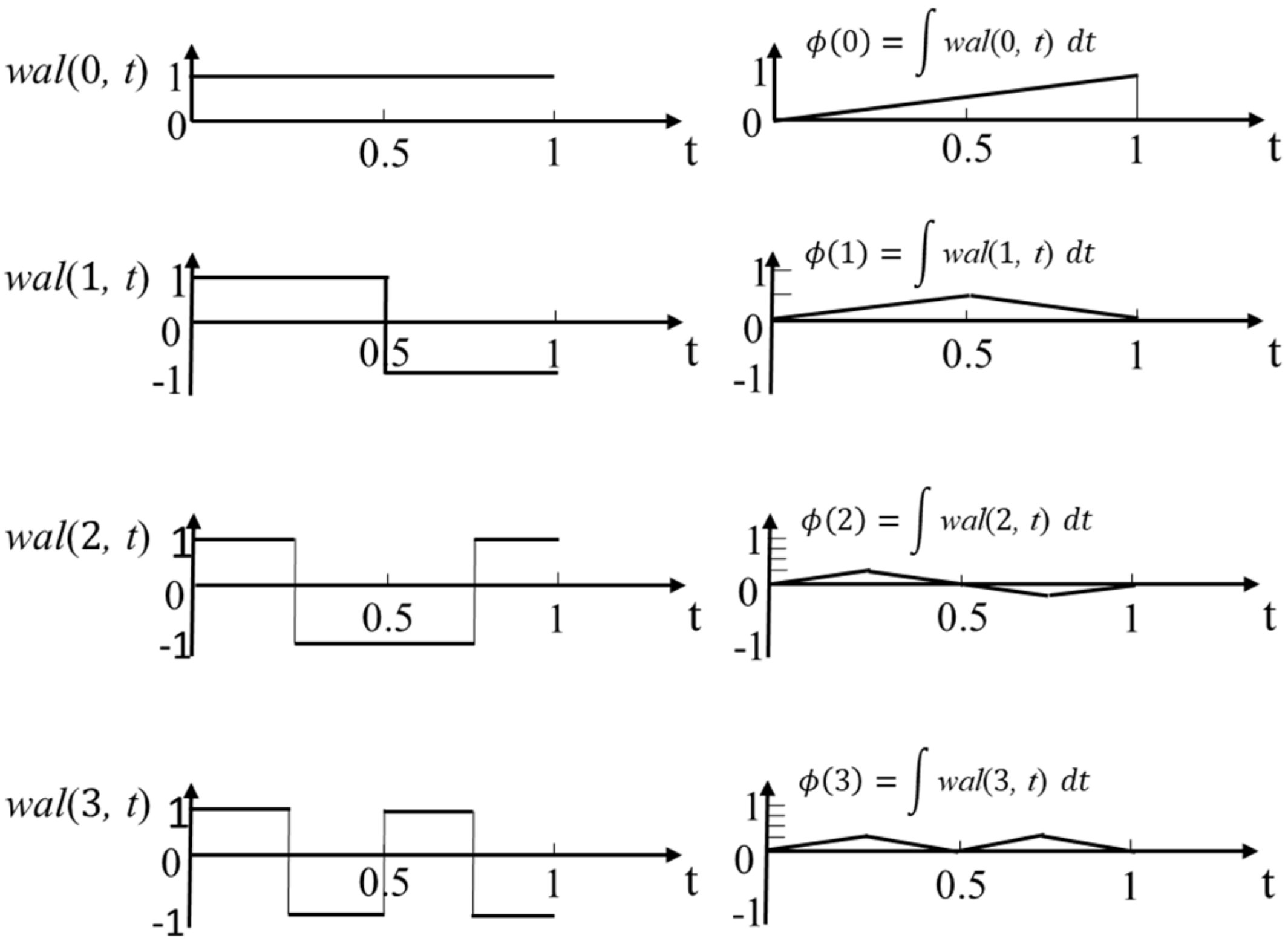
2.1. Walsh Series and Transform

The Walsh series is a family of non-sinusoidal orthogonal rectangular functions, originally defined by Walsh in 1923 [24,25]. Figure 1 shows the first eight Walsh series. Each function in the Walsh series, of different orders, jumps from 1 to −1 within the interval [0, 1] [26]. They are orthogonal, symmetrical and linear, thus extremely suitable for signal reconstruction [27], but only a few studies in literature have addressed their applicability to the recovery of random series.

In digital processing, the discrete Walsh transform (DWT) and the inverse DWT (IDWT) of a signal x(t) in terms of the Walsh series wal(k, n) are defined as [28]:

$$X\left(k\right)=\frac{1}{N}{\displaystyle \sum }_{n=0}^{N-1}x\left(n\right)wal\left(k,n\right);k=0,1,2,\dots ,N-1$$

(1)

$$x\left(n\right)={\displaystyle \sum }_{k=0}^{N-1}X\left(k\right)wal\left(k,n\right);n=0,1,2,\dots ,N-1$$

(2)

2.2. Walsh Transform Versus Fourier Transform

Unlike the Fourier transform, the Walsh transform is operated by real number additions and subtractions. Walsh functions are formed in rectangular waveforms of ±1 that are piecewise constant. This characteristic makes the calculations much less complicated, as opposed to complex number handling in FFT [29,30]. Moreover, all Walsh functions are arranged by a certain order and in constant formations (Figure 1). Their shapes are invariable regardless of the selected order number k for a given random signal. As a result, the stability of the integral result is guaranteed. On the contrary, the Fourier transform aims to convert a signal into a trigonometric series whose frequencies, amplitudes and corresponding resolution depend on the sample number N used in FFT. In addition, in accordance with the Nyquist-Shannon sampling theorem [31], the Nyquist folding frequency fc in FFT is determined by the time interval Δt. Aliasing of components higher than fc into the spectral zone of f < fc is inevitable. Hence, selections of parameters would significantly influence the integral results [17].

2.3. Empirical Mode Decomposition (EMD)

The Empirical Mode Decomposition (EMD) method is adopted in the WATEBI algorithm for removing the nonlinear noise in the reconstructed velocity and displacement. The EMD method was proposed by Huang et al. [32]. The vibration signal can be decomposed into several intrinsic mode functions (IMF) and a residual term shown as Equation (3).

$$x\left(t\right)=IMF\left[x\left(t\right)\right]+RS\left[x_r\left(t\right)\right]$$

(3)

where IMF[x(t)] are the intrinsic mode functions and RS[x_r(t)] is the residual term.

It is suggested that the remnant RS[x_r(t)] of a signal serving as random inutile residue be discarded after the Hilbert-Huang transform [32,33,34]. Thus, the last term of EMD is removed from the velocity and displacement signal in the WATEBI method.

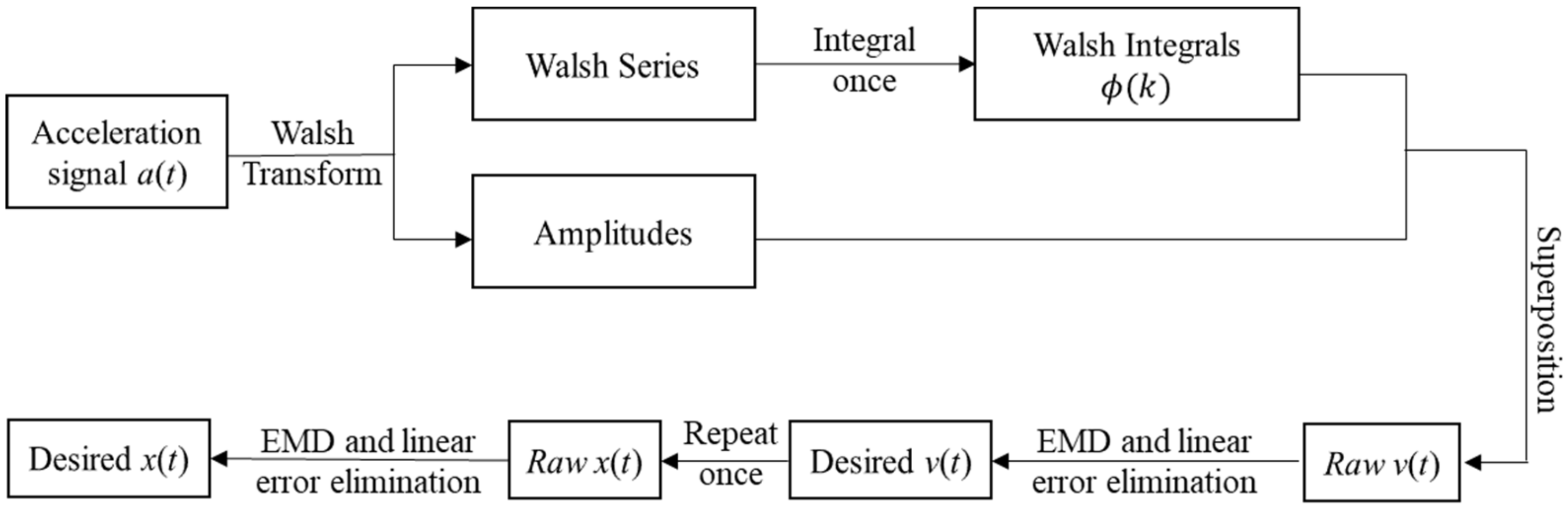
2.4. Signal Reconstruction

A digital time history of acceleration can be first transformed into N-order Walsh series as follows.

$$a\left(n\right)={\displaystyle \sum }_{k=0}^{N-1}A\left(k\right)wal\left(k,n\right);n=0,1,2,\dots ,N-1$$

(4)

where a(n) is the varying acceleration at time instant of (n-1)Δt, Δt is the equidistant time interval. The velocity is then obtained by integration of the right-hand-side (RHS) once, despite that its initial condition might be unknown.

$$v\left(n\right)=\Delta t{\displaystyle \sum }_{m=0}^{m=n}{\displaystyle \sum }_{k=0}^{N-1}A\left(k\right)wal\left(k,m\right)={\displaystyle \sum }_{k=0}^{N-1}A\left(k\right)\varphi \left(k\right);n=0,1,2,\dots ,N-1$$

(5)

where

$$\varphi \left(k\right)={\displaystyle \sum }_{m=0}^{m=n}wal\left(k,m\right)\Delta t$$

is the discrete version of the integral of Walsh series [27]. Figure 2 illustrates the first four integrals of Walsh series. Obviously, they are triangles and linear.

The derivation of displacement follows the same steps as velocity.

$$v\left(n\right)={\displaystyle \sum }_{k=0}^{N-1}V\left(k\right)wal\left(k,n\right); n=0,1,2,\dots ,N-1$$

(6)

$$x\left(n\right)={\displaystyle \sum }_{k=0}^{N-1}V\left(k\right){\displaystyle \sum }_{m=0}^{m=n}wal\left(k,m\right)\Delta t={\displaystyle \sum }_{k=0}^{N-1}V\left(k\right)\varphi \left(k\right);n=0,1,2,\dots ,N-1$$

(7)

A(k) and V(k) in Equations (4) and (6) are respective Walsh coefficients of acceleration and velocity, indicating the amplitudes of Walsh series in Figure 1. These two equations both involve integrals of wal(k, n) that are identical and therefore need to be computed only once. A 2-dimensional N-by-N matrix can be used to store them beforehand. Apparently, the above algorithm is numerically simple and fast as it only requires superposition of the integrals of series wal(k, n) with respective coefficients for k = 0, 1, …, N − 1 that can be easily fulfilled by matrix manipulations. In this study, the MATLAB-based Hadamard-Walsh transform [35] is used to obtain the Walsh coefficients. The residual noise in the discrete velocity and displacement is then removed by the EMD method respectively.

Figure 3 illustrates the procedures of implementing WATEBI algorithm.

2.5. Numerical Effectiveness and Elimination of Trend Error

It should be noted that the amplitude, namely coefficient A(k) or V(k), of a high-order Walsh series is very small, such that the corresponding integral contributes little to the overall displacement. Additionally, analogous to Fourier series, high-frequency components in the original signal are usually regarded as noise that ought to be filtered off. Therefore, in the WATEBI algorithm, only the low-order series are retained for use. By doing so, the computational time is reduced by approximately half as well. In general, the first half of Walsh series suffices the accuracy requirement while the second half are truncated, i.e.

$$A\left(k\right)=V\left(k\right)=0; k=\frac{N}{2},\frac{N}{2}+1,\dots ,N-1$$

(8)

Considering that this WATEBI algorithm only uses first-order integrals of Walsh series in the linear formation, the accumulation of integral errors of the derived velocity is insignificant.

For displacement, although the linear superposition of Walsh series is performed for one more time, the integral kernels in Figure 2 are unchanged. Hence, the accumulated error is one order lower than the square term from conventional time-domain integration methods. Nevertheless, the trend error still exists and should be removed in order to eliminate its subsequent influence on the displacement. In this study, the least-squares method is employed to fit the linear term in trend error of velocity and displacement.

3. Case Studies and Analyses

To assess the performance of the proposed WATEBI method, three case studies are presented in this paper. These are vibration of a SDOF system and the ground motions of El Centro earthquake and Kaikoura earthquake. In each case study, the WATEBI method is compared with time-domain trapezoidal integral by Labview [36], MATLAB Ode45 (Ordinary Differential Equation) function with tolerance of 10⁻⁶ [37], low-frequency cutoff [18], and low-frequency attenuation with the target accuracy α_T = 0.97 [16,17]. For a fair comparison among all methods, both the linear trend in velocity and the nonlinear trend in displacement have been removed, respectively by linear fitting and nonlinear fitting. The only difference is that the WATEBI method employs EMD while the benchmark methods use the common least-squares method.

Please note that the attenuation algorithm in reference [16] is only given for displacement. The accuracy of the frequency domain methods (low-frequency cutoff [18] and low-frequency attenuation [16,17]) heavily depends upon parameter selection. In this paper, the parameters in the selected frequency domain methods for all three case studies are tuned to obtain the ideal results. In Case 1, the cut-off frequency in the cutoff method and the target frequency in the attenuation method are 0.1 Hz, coincidently. In Case 2, they are 0.07 Hz and 0.1 Hz respectively. In Case 3, they coincide again at 0.15 Hz.

In each case study, the following three indicators are used to evaluate the deviation of the reconstructed signal away from the reference velocity/displacement.

(1) Average peak error Er₁, which denotes the average deviation at both positive and negative extremes of the time series, is defined as

$$E{r}_{peak}{}^{+}=\left|\frac{\mathit{max}[X\left(t\right)\left]-\mathit{max}[x\left(t\right)\right]}{\mathit{max}[x\left(t\right)]}\right|, E{r}_{peak}{}^{-}=\left|\frac{\mathit{min}[X\left(t\right)\left]-\mathit{min}[x\left(t\right)\right]}{\mathit{min}[x\left(t\right)]}\right|$$

(9)

where x(t) is the reference signal and X(t) is the reconstructed signal.

$$E{r}_1=\frac{1}{2}\left(E{r}_{peak}{}^{+}+E{r}_{peak}{}^{-}\right)$$

(10)

(2) Maximum peak error Er₂, denoting the larger deviation at positive and negative extremes of the time series, which is often the most concerned and useful information for comparison.

$$E{r}_2=\mathit{max}(E{r}_{peak}{}^{+},E{r}_{peak}{}^{-})$$

(11)

(3) Root-mean-square error Er₃ represents the overall deviation of the whole time series at every time instants.

$$E{r}_3=\sqrt{\frac{{{\displaystyle \sum }}_{i=0}^{N-1}{(x\left(t_i\right)-X\left(t_i\right))}^2}{N}}$$

(12)

3.1. Case 1: Vibration of a SDOF System

A SDOF vibration system driven by white noise is considered first.

$$M\cdot a\left(t\right)+C\cdot v\left(t\right)+K\cdot x\left(t\right)=-F\left(t\right)$$

(13)

where x, v and a are respectively displacement, velocity and acceleration of system vibration. The assumed frequency of excitation F ranges from 0.1 Hz to 5.1 Hz and its power spectrum is constant, 1 N²s. Mean of F is zero. The SDOF system has a vibration mass M of 1 kg, natural frequency f_n of 0.45 Hz and damping ratio of 3%. The initial velocity and displacement are assumed as 0 cm/s and −3.2 cm.

The dynamic responses including acceleration, velocity and displacement are solved by the Newmark-β method of β = ¼ [38]. This method is stepwise and has been widely applied in civil engineering for years due to its accuracy, as long as a suitable interval Δt is chosen in computation. This study uses a small time interval, Δt = 0.0586 s. Figure 4 shows the time-domain numerical solution of excited acceleration for duration of 239.94 s.

Figure 5a shows the velocities reconstructed by the five methods against the reference velocity solved by the Newmark-β method. The comparison of displacements is given in Figure 6a. In these two figures, it can be clearly seen that after removal of trend by fittings, none of the reconstructed signals contains drift. Moreover, at the beginning and ending parts of the full duration, these two frequency domain methods fail to precisely reconstruct both velocity and displacement. By contrast, as illustrated in the enlarged details in Figure 5b and Figure 6b, the velocity and displacement reconstructed by the WATEBI method match the reference time series with smallest deviations.

The comparisons of average peak, maximum peak error and root-mean-square error for the underlying five methods are given in

Table 1. Five methods for the velocity reconstruction of SDOF system.

Algorithms	Average Peak Error (%)	Maximum Peak Error (%)	Root-Mean-Square Error
Trapezoidal integral	0.32	0.33	0.12
Matlab Ode45	0.05	0.05	0.01
Low-frequency cutoff	0.83	0.91	0.04
Low-frequency attenuation	-	-	-
WATEBI	0.43	0.57	0.02

and

Table 2. Five methods for the displacement reconstruction of SDOF system

Algorithms	Average Peak Error (%)	Maximum Peak Error (%)	Root-Mean-Square Error
Trapezoidal integral	0.21	0.26	0.07
Matlab Ode45	0.39	0.6	0.01
Low-frequency cutoff	0.4	0.47	0.04
Low-frequency attenuation	10.85	21.43	0.12
WATEBI	0.19	0.23	0.02

, respectively for velocity and displacement. It can be shown from the three error indicators that for velocity the low-frequency cutoff method performs worst, while for displacement the low-frequency attenuation is of lowest accuracy. For both velocity and displacement, the best performance among all five methods is WATEBI. In addition, the good performances of Matlab Ode45 and trapezoidal integral are noticeable, because they are analogous to the Newmark-β algorithm for the adopted step-by-step integration scheme in the time domain and actually in this SDOF system no noise is contained in the acceleration signal. Nonetheless, in the following case studies, the limitation and drawback of time-domain methods will be demonstrated when random noise is mixed in the acceleration.

3.2. Case 2: El Centro Earthquake Ground Motion

The El Centro earthquake ground motion, widely used in civil and earthquake engineering, was obtained from the Imperial Valley earthquake in 1940, recorded at the site of El Centro. The acceleration record is a 2688-point signal with Δt = 0.02s. It can be seen from Figure 7a that the maximum ground motion exceeds 300 Gal (cm/s²). Figure 7b shows the amplitude spectrum of acceleration. Obviously, it is wide-banded, and contains numerous frequency components as many other seismic records do and the frequencies of significant components are lower than 10 Hz. Noise may exist in the record due to low-frequency tilt of device, high frequency burr or even direct component, all possibly leading to deviation in the reconstructed velocity and displacement.

The site-recorded velocity and displacement are used as reference for assessing the accuracy of WATEBI algorithm. Before running WATEBI, the original acceleration history is interpolated with the cubic spline function using Δt/6, in order to achieve a finer and smoother curve.

Although the original ground motion of acceleration is stochastic and transient, it can be seen from Figure 8 and Figure 9 that the reconstructed signals (especially velocity) by WATEBI approach more closely to the site records than the other four methods do. For displacement, the deviation from the real data starts at some 35 s, but the two most useful peak-to-trough cycles (from 12 s to 28 s) for checking structural dynamic responses are well matched.

Table 3. Five methods for the velocity reconstruction of El Centro event.

Algorithms	Average Peak Error (%)	Maximum Peak Error (%)	Root-Mean-Square Error
Trapezoidal integral	1.63	1.68	0.51
Matlab Ode45	3.86	7.04	1.05
Low-frequency cutoff	3.33	6.42	0.64
Low-frequency attenuation	-	-	-
WATEBI	1.47	2.47	0.32

and

Table 4. Five methods for the displacement reconstruction of El Centro event.

Algorithms	Average Peak Error (%)	Maximum Peak Error (%)	Root-Mean-Square Error
Trapezoidal integral	6.81	12.55	0.77
Matlab Ode45	7.98	13.87	1.15
Low-frequency cutoff	11.04	11.09	1.33
Low-frequency attenuation	11.73	12.41	1.23
WATEBI	5.93	8.71	0.74

compares the performance of five methods for numerically derived velocity and displacement. It is obvious that the trapezoidal integral is still efficient in velocity reconstruction, with regard to error control on peaks, but for the overall performance of velocity and displacement, the proposed WATEBI method outruns all the rest four methods. It should be also recognized that the three error evaluating indicators (Equations (10)–(12)) of displacement results are larger than those of the velocity results. After all, displacement reconstruction is based on velocity. Both noise and the tiny trend term in velocity can amplify the deviation in displacement.

3.3. Case 3: Kaikoura Earthquake in The South Island of New Zealand

The Kaikoura earthquake that occurred in the South Island of New Zealand on 13 November 2016 was a very strong seismic event with magnitude of 7.8 (M_w) and a long duration of approximately two minutes. The seismic data used in this paper is a horizontal component that has been corrected after occurrence. The data was recorded with a constant time interval of 0.005 s. Figure 10 shows the time history of acceleration and its amplitude spectrum. Compared with the El Centro record in Figure 7, the energy of Kaikoura record is more concentrated, not only for time history but also for spectrum.

Owing to the fine time interval, the total number of logging is 14,327, such that interpolation of data is unnecessary. The reconstructions by WATEBI only require seconds of computational time, using an ordinary computer. Figure 11 and Figure 12 illustrate the waveforms of original and derived velocity and displacement. The good performance of WATEBI algorithm is again demonstrated. The low-frequency cutoff method shows the worst degree of reconstruction among all methods, especially in displacement. Considering that more and more advanced technologies have been applied in earthquake monitoring, rich and accurate seismic recordings are available. This in turn helps to improve the accuracy in deriving velocity and displacement in terms of acceleration. Therefore, very good agreement between the derived and recorded data can be expected.

Table 5. Five methods for the velocity reconstruction of Kaikoura event.

Algorithms	Average Peak Error (%)	Maximum Peak Error (%)	Root-Mean-Square Error
Trapezoidal integral	0.33	0.65	1.68
Matlab Ode45	0.32	0.51	0.10
Low-frequency cutoff	1.77	2.46	1.38
Low-frequency attenuation	-	-	-
WATEBI	1.04	1.94	0.75

and

Table 6. Five methods for the displacement reconstruction of Kaikoura event.

Algorithms	Average Peak Error (%)	Maximum Peak Error (%)	Root-Mean-Square Error
Trapezoidal integral	0.63	0.69	0.61
Matlab Ode45	2.17	2.45	0.77
Low-frequency cutoff	4.35	7.80	1.58
Low-frequency attenuation	0.91	0.96	0.12
WATEBI	0.64	0.73	0.35

give the comparison of five methods in deriving the velocity and displacement of Kaikoura earthquake. Again, the three error indicators show that the proposed WATEBI algorithm is most robust. For displacement, both the average peak error and the maximum peak error by WATEBI are even below 1%. The low-frequency attenuation method also provides good accuracy, because the target frequency has been tuned according to the target accuracy α_T = 0.97. By contrast, the low-frequency cutoff is the worst among all five methods, not only for velocity but also displacement.

4. Concluding Remarks

Accelerometers are usually employed to measure vibration signals in engineering practice. To numerically derive random velocity and displacement from recorded acceleration, a Walsh Transform and Empirical Mode Decomposition (EMD)-based integral algorithm, WATEBI in short, is proposed in this study. It is actually the linear superposition of the integral kernels of Walsh series and can be handled by an ordinary computer with ease. The residual noise in the reconstructed vibration signals is eliminated by EMD. Unlike the popularly used low-frequency cutoff and low-frequency attenuation methods, this algorithm does not need to specify the critical parameters like cutoff frequency, target frequency and target accuracy. As shown in the flowchart (Figure 3), the trend term is removed by linear least-squares fit.

To test the performance of the WATEBI algorithm, three distinct case studies are used. They are respectively the vibration of a SDOF system with given parameters, ground motions of El Centro earthquake and Kaikoura earthquake. In each case study, all reference velocity and displacement are available. Then for the comparison among five methods, trapezoidal integral, Matlab Ode45, low-frequency cutoff, low-frequency attenuation and WATEBI, the reconstructed signals of velocity and displacement are investigated. The average peak error, the maximum peak error and the root-mean-square error, are three criterions used to differentiate the level of quality of these methods. The graphical comparisons of both full duration and enlarged details in Figure 5, Figure 6, Figure 8, Figure 9, Figure 11 and Figure 12 reveal that not only the time history of reconstructed velocity by WATEBI perfectly overlaps the reference signal, but also the reconstructed displacement by WATEBI tallies with the reference data with very little deviations, especially at peaks and troughs. The errors in Table 1, Table 2, Table 3, Table 4, Table 5 and Table 6 also demonstrate that for both velocity and displacement, the overall performance of WATEBI is the best among all compared methods. Particularly for displacement, WATEBI behaves very stably, providing lowest errors for all three cases. The Ode45 algorithm works very well in Case 1 and Case 3 for velocity reconstruction, while the trapezoidal integral method is suitable for all cases. The low-frequency cutoff method gives accurate velocity only in Case 1, while the low-frequency attenuation method renders accurate displacement in Case 3. Nevertheless, none of these four methods surpass the WATEBI algorithm in nearly all cases. Additionally, the WATEBI algorithm is more adaptive, since, as depicted in the flowchart (Figure 3), the signal reconstruction does not require subjective parameters such as cutoff and target frequencies to be specified. Signals adopted in these cases are equally spaced. However, for the irregularly sampled data series, the ALLSSA method might be more robust for the preprocessing than higher-order spline methods.

The merit of Walsh transform with constant kernels has inspired this research work. For the sake of limited length of this paper, many other case studies to validate the robustness of the proposed algorithm are not included. Different from the long and popularly used Fourier transform and Hilbert transform in signal processing, the Walsh transform still looks like a stranger to many researchers. Hopefully more virtues of the Walsh transform could be rediscovered to further invoke its wider application in engineering problems.

References

1. Zhou, Y.J. A Study on Integral Algorithm for Acceleration Test to Get Displacement and Application. Master’s Thesis, Chongqing University, Chongqing, China, 2013. [Google Scholar]
2. Housner, G.; Bergman, L.A.; Caughey, T.K.; Chassiakos, A.G.; Claus, R.O.; Masri, S.F.; Skelton, R.E.; Soong, T.; Spencer, B.; Yao, J.T. Structural control: Past, present, and future. J. Eng. Mech. 1997, 123, 897–971. [Google Scholar] [CrossRef]
3. Smyth, A.; Wu, M. Multi-rate Kalman filtering for the data fusion of displacement and acceleration response measurements in dynamic system monitoring. Mech. Syst. Signal Pr. 2007, 21, 706–723. [Google Scholar] [CrossRef]
4. Gutenberg, B.; Richter, C.F. Earthquake magnitude, intensity, energy, and acceleration. Bull. Seismol. Soc. Am. 1942, 32, 163–191. [Google Scholar]
5. Berg, G.; Housner, G. Integrated velocity and displacement of strong earthquake ground motion. Bull. Seismol. Soc. Am. 1961, 51, 175–189. [Google Scholar]
6. Li, Q.; Wang, T.; Xu, Y. The Modification of the Vibration Parameter Transform Based on Frequency Domain Integration. Modular. Mach. T. Auto. Man. Tec. 2005, 9, 60–61. [Google Scholar]
7. Hamming, R.W. Digital Filters, 3rd ed.; Prentice-Hall: Englewood Cliffs, NJ, USA, 1989. [Google Scholar]
8. Wang, G.Q.; Boore, D.M.; Igel, H.; Zhou, X.Y. Some observations on colocated and closely spaced strong ground-motion records of the 1999 Chi-Chi, Taiwan, earthquake. Bull. Seismol. Soc. Am. 2003, 93, 674–693. [Google Scholar] [CrossRef] [Green Version]
9. Cooley, J.W.; Tukey, J.W. An algorithm for the machine calculation of complex Fourier series. Math. Comput. 1965, 19, 297–301. [Google Scholar] [CrossRef]
10. Ghaderpour, E.; Liao, W.; Lamoureux, M.P. Antileakage least-squares spectral analysis for seismic data regularization and random noise attenuation. Geophysics 2018, 83, 157–170. [Google Scholar] [CrossRef]
11. Ghaderpour, E. Multichannel antileakage least-squares spectral analysis for seismic data regularization beyond aliasing. Acta Geophys. 2019, 67, 1349–1363. [Google Scholar] [CrossRef]
12. Xu, S.; Zhang, Y.; Pham, D.; Lambaré, G. Antileakage Fourier transform for seismic data regularization. Geophysics 2005, 70, 87–95. [Google Scholar] [CrossRef]
13. Guo, J.; Zheng, Y.; Liao, W. High fidelity seismic trace interpolation. In Proceedings of the SEG Annual Meeting, New Orleans, LA, USA, 18–23 October 2015. [Google Scholar]
14. Zhou, X.X.; Chen, E.K.; lv, G.Q.; Liu, L.X. The Processing of Vibration Acceleration Signal Based on Numerical Integration and LMS. Process. Autom. Instrum. 2006, 9, 51–53. [Google Scholar]
15. Park, K.T.; Kim, S.H.; Park, H.S.; Lee, K.W. The determination of bridge displacement using measured acceleration. Eng. Struct. 2005, 27, 371–378. [Google Scholar] [CrossRef]
16. Lee, H.S.; Hong, Y.H.; Park, H.W. Design of an FIR filter for the displacement reconstruction using measured acceleration in low-frequency dominant structures. Int. J. Numer. Meth. Eng. 2009, 82, 403–434. [Google Scholar] [CrossRef]
17. Hong, Y.H.; Kim, H.K.; Lee, H.S. Reconstruction of dynamic displacement and velocity from measured accelerations using the variational statement of an inverse problem. J. Sound Vib. 2010, 329, 4980–5003. [Google Scholar] [CrossRef]
18. Wang, J.; Hu, X. Application of Matlab in Processing of Vibration Signals; China Water & Power Press: Beijing, China, 2006. [Google Scholar]
19. Huang, N.E.; Shen, S. Hilbert-Huang Transform and Its Applications; World Scientific: Singapore, 2014. [Google Scholar]
20. Huang, N.E.; Attoh-Okine, N.O. The Hilbert-Huang Transform in Engineering; CRC Press: Boca Raton, FL, USA, 2005. [Google Scholar]
21. Daubechies, I. The wavelet transform, time-frequency localization and signal analysis. IEEE Trans. Inform. Theory 1990, 36, 961–1005. [Google Scholar] [CrossRef] [Green Version]
22. Peng, Z.; Peter, W.T.; Chu, F. A comparison study of improved Hilbert-Huang transform and wavelet transform: Application to fault diagnosis for rolling bearing. Mech. Syst. Signal Pr. 2005, 19, 974–988. [Google Scholar] [CrossRef]
23. Ghaderpour, E.; Pagiatakis, S.D. LSWAVE: A MATLAB software for the least-squares wavelet and cross-wavelet analyses. GPS Solut. 2019, 23, 50. [Google Scholar] [CrossRef]
24. Walsh, J.L. A closed set of normal orthogonal functions. Am. J. Math. 1923, 45, 5–24. [Google Scholar] [CrossRef] [Green Version]
25. Horadam, K.J. Hadamard Matrices and Their Applications; Princeton University Press: Princeton, NJ, USA, 2012. [Google Scholar]
26. Beauchamp, K.G. Walsh Functions and Their Applications; Academic Press: Cambridge, MA, USA, 1975. [Google Scholar]
27. Corrington, M. Solution of differential and integral equations with Walsh functions. IEEE Trans. Circuit Theory 1973, 20, 470–476. [Google Scholar] [CrossRef]
28. Aloui, N.; Bousselmi, S.; Cherif, A. Speech Compression Based on Discrete Walsh Hadamard Transform. Int. J. Inform. Eng. Electron. Bus. 2013, 5, 59. [Google Scholar] [CrossRef] [Green Version]
29. Ashrafi, A. Walsh–Hadamard Transforms: A Review. Adv. Imag. Elect. Phys. 2017, 201, 1–55. [Google Scholar]
30. Jayathilake, A.A.C.A.; Perera, A.A.I.; Chamikara, M.A.P. Discrete Walsh-Hadamard transform in signal processing. Int. J. Res. Inf. Technol. 2013, 1, 80–89. [Google Scholar]
31. Press, W.H. The Art of Scientific Computing; Cambridge University Press: Cambridge, UK, 1992. [Google Scholar]
32. Huang, N.E.; Shen, Z.; Long, S.R.; Wu, M.C.; Shih, H.H.; Zheng, Q.; Yen, N.C.; Tung, C.C.; Liu, H.H. The empirical mode decomposition and the Hilbert spectrum for nonlinear and non-stationary time series analysis. Proc. R. Soc. A Math. Phys. 1998, 454, 903–995. [Google Scholar] [CrossRef]
33. Rilling, G.; Flandrin, P.; Goncalves, P. On empirical mode decomposition and its algorithms. Proceedings of IEEE-EURASIP Workshop on Nonlinear Signal and Image Processing NSIP-03, Grado, Italy, 8–11 June 2003. [Google Scholar]
34. Flandrin, P.; Rilling, G.; Goncalves, P. Empirical mode decomposition as a filter bank. IEEE Signal Proc. Lett. 2004, 11, 112–114. [Google Scholar] [CrossRef] [Green Version]
35. Hahn, B. Essential MATLAB for Scientists and Engineers, 3rd ed.; Pearson Education: Cape Town, South Africa, 2002. [Google Scholar]
36. Travis, J.; Kring, J. LabVIEW for Everyone; Prentice-Hall: Upper Saddle River, NJ, USA, 2007. [Google Scholar]
37. Lindfield, G.; Penny, J. Numerical Methods: Using MATLAB, 4th ed.; Academic Press: London, UK, 2018. [Google Scholar]
38. Newmark, N.M. A method of computation for structural dynamics. J. Eng. Mech. Div. 1959, 85, 67–94. [Google Scholar]
Figure 1. Illustration of first eight Walsh series adapted from [27].
Applsci 10 03509 g001
Figure 2. The first four integrals of Walsh functions adapted from [27].
Applsci 10 03509 g002
Figure 3. The flowchart of the Walsh transform and Empirical Mode Decomposition-based integral (WATEBI) algorithm.
Applsci 10 03509 g003
Figure 4. Simulated acceleration time history of single-degree-of-freedom (SDOF) system.
Applsci 10 03509 g004
Figure 5. Velocity of the SDOF system: (a) Full duration; (b) Enlarged detail at the tail end.
Applsci 10 03509 g005
Figure 6. Displacement of the SDOF system: (a) Full duration; (b) Enlarged detail at the tail end.
Applsci 10 03509 g006
Figure 7. Recorded acceleration of El Centro earthquake: (a) Acceleration time history; (b) Amplitude spectrum.
Applsci 10 03509 g007aApplsci 10 03509 g007b
Figure 8. Velocity of El Centro ground motion: (a) Full duration; (b) Enlarged detail at largest trough.
Applsci 10 03509 g008aApplsci 10 03509 g008b
Figure 9. Displacement of El Centro ground motion: (a) Full duration; (b) Enlarged detail at largest peak.
Applsci 10 03509 g009aApplsci 10 03509 g009b
Figure 10. Recorded acceleration of Kaikoura earthquake: (a) Full time history; (b) Amplitude spectrum.
Applsci 10 03509 g010
Figure 11. Velocity of Kaikoura ground motion: (a) Full duration; (b) Enlarged detail at largest trough.
Applsci 10 03509 g011
Figure 12. Displacement of Kaikoura ground motion: (a) Full duration; (b) Enlarged detail at largest trough.
Applsci 10 03509 g012aApplsci 10 03509 g012b