Efficient Distributed Preprocessing Model for Machine Learning-Based Anomaly Detection over Large-Scale Cybersecurity Datasets

Abstract

New computational and technological paradigms that currently guide developments in the information society, i.e., Internet of things, pervasive technology, or Ubicomp, favor the appearance of new intrusion vectors that can directly affect people’s daily lives. This, together with advances in techniques and methods used for developing new cyber-attacks, exponentially increases the number of cyber threats which affect the information society. Because of this, the development and improvement of technology that assists cybersecurity experts to prevent and detect attacks arose as a fundamental pillar in the field of cybersecurity. Specifically, intrusion detection systems are now a fundamental tool in the provision of services through the internet. However, these systems have certain limitations, i.e., false positives, real-time analytics, etc., which require their operation to be supervised. Therefore, it is necessary to offer architectures and systems that favor an efficient analysis of the data handled by these tools. In this sense, this paper presents a new model of data preprocessing based on a novel distributed computing architecture focused on large-scale datasets such as UGR’16. In addition, the paper analyzes the use of machine learning techniques in order to improve the response and efficiency of the proposed preprocessing model. Thus, the solution developed achieves good results in terms of computer performance. Finally, the proposal shows the adequateness of decision tree algorithms for training a machine learning model by using a large dataset when compared with a multilayer perceptron neural network.

1. Introduction

The inclusion of computational elements into the daily life of people, i.e., Internet of things, wearable technology, or Ubicomp, applied to a sensitive user context such as healthcare, offers new intrusion vectors that directly affects people’s lives [1]. Currently, the use of sophisticated techniques and technology to develop new and more efficient cyber-attacks is exponentially increasing the number of cyber-threats

The improvement of methods for preventing and detecting cyberattacks acquired great importance, increasing the impact on technological developments and becoming a fundamental pillar of the digital era. In this sense, the integration of artificial intelligence (AI) in the context of cybersecurity favored this necessary improvement [2]. The integration of AI and cybersecurity can be applied to different cybersecurity systems, i.e., to prioritize events using resilient incident response platforms in Security Operation Center (SOCs), to automatize security analysis, or to detect and predict threats before they materialize. The integration of AI can be especially positive in intrusion detection systems (IDSs), which process a huge amount of network traffic from Internet of things (IoT), wearables, wireless sensors, host–host-based sensors, and network computing.

IDSs are software systems that monitor and analyze the behavior of networks and systems with the objective of detecting some possible intrusion. There are two classes of IDSs: those based on signature detection and those based on anomaly detection. IDSs that are based on signature detection apply different rules to detect an attack over a network or a host. Alternatively, an anomaly-based detection IDS can differentiate between normal and anomalous flow. However, the problem of false alarms (false positives) is a major concern in the use of IDS [3], which consequently leads to the need for an expert in cybersecurity to evaluate the results and investigate the veracity of these false positives [4]. This process takes a considerable amount of time with a need for qualified people.

Technology and techniques used to implement IDSs are mostly publicly known; thus, attackers are always improving their methods, trying to find a way to bypass IDSs without being detected [5]. This led to the materialization of a new generation of IDSs which, through the use of AI, try to improve their efficiency and effectiveness via anomaly-based IDS.

Nevertheless, many of these research works were usually based on KDD’99 and DARPA datasets, which have twenty years of history and do not represent the current state of the art of systems, attacks, and cybersecurity [6,7,8,9]. These datasets are small and do not represent large-scale data compared with other recent datasets such as UGR’16 [10]. In Reference [11], there is a representation of the most used datasets in the last decade for machine learning applications related to intrusion detection. For instance, DARPA 98, DARPA 99, and DARPA 2000 datasets [12] constituted 8.6% of usage and the GureKddcup dataset [13] constituted 1.4%, a percentage shared by the ISCX2012 dataset [14] and UNB-CIC [15]. Other used datasets are NSL-KDD [16] with 11.6% of usage, KDD-99 [17] with 63.8% of usage, and finally generated and simulated datasets with 11.6%. These datasets mentioned above do not represent the current state of the art related to information security.

In recent years, AI and specifically machine learning (ML) techniques were implemented to solve problems related to anomaly-based IDSs, in order to improve attack detections. However, training ML-based IDSs is costly in terms of time and computational requirements due to the large amount of data needed to be processed.

The use of ML methods for developing a better IDS is a trending research topic which provided good results. Nevertheless, some stages of the ML process must be optimized, such as data preparation (preprocessing), to obtain good results in terms of accuracy. To achieve an optimal preprocessing model for large-scale datasets, a new model of preprocessing and training IDS with a truly large dataset is presented in this research.

This paper introduces a new way to preprocess large-scale datasets focused on IDSs as presented in Section 2. Furthermore, in Section 3, Section 4 and Section 5, we explain the problem statement and the proposed methodology, defining the new architecture presented in this paper, oriented to data preprocessing. These sections also include the architecture proposed for applying the multilayer perceptron (MLP) and decision trees in anomaly-based IDSs. Section 6 and Section 7 provide the obtained results after applying our proposal to large-scale datasets. For our tests, we used the UGR’16 dataset, as well as a comparison with its execution locally, concluding with a comparison of ML algorithms such as deep learning and non-deep learning algorithms, i.e., MLP and decision tree, respectively.

2. Related Work

Currently, there are several approaches of how to apply ML to cybersecurity based on a network sensor response, specifically for intrusion detection. These different approaches consider diverse parameters such as the classification of the attacks, network flow variables that should be included, solutions based on data mining, or solutions directly based on various ML algorithms with the aim of finding the best model.

In Reference [5], the authors established the basis of intrusion detection systems. In that work, one of the main contributions was defining how IDSs should work in order to detect more attacks easily by analyzing the detecting mechanism. Another contribution was a classification of the different attacks. As stated, by establishing the differences between the types of attacks, the detection mechanism can be fine-tuned, ending in a better detection. In addition, those researchers tried giving an approach to a good ML model for IDSs by using different techniques. In those studies, the best results were achieved by neural networks, closely followed by decision trees and nearest neighbor.

Following the approach started by Reference [5], the authors of Reference [18] tried going deeper with the objective of proposing a model with optimal parameters for neural networks. Their research was based on previous works that, however, did not reach truly optimal models. To solve this problem, they adopted an approach based on a five-stage model with the aim of studying the majority of possibilities. This approach specifies a comparison to get the best parameters related to the best dataset features and the way that those features must be normalized to get the best of them. Furthermore, they specified the way in which the neural network must be built having to account for the number of hidden layers, the number of nodes inside each one of the layers, the activation function, and some other parameters for the best adjustment of the neural network. Afterward, the research made a comparison with a combination of different solutions, whether proposed by them or by other researchers. The conclusion was clear; they identified the best activation function to be used rectified linear unit (ReLU), the formula to calculate the architecture of the neural network model, and how to normalize each type of data included in the dataset. The rules defined are shown in Equations (1) [19], (2) [20], (3), and (4) [21], where H is the number of hidden layers of an IDS, input is the number of entries, and output is the number of exits in the neural network model.

H = 0.75 × Input + Output,

(1)

H = (Input + Output)/2,

(2)

H = Input × 70%,

(3)

H = Input × 90%.

(4)

Different approaches were presented using techniques such as Apache Spark to improve the preprocessing of the dataset and its performance [5,7,22]. However, the used datasets cannot be currently considered as large-scale and did not include real background traffic.

The most common dataset used in nearly all the studies analyzed is KDD’99, as mentioned before in Section 1. KDD’99 is a dataset that includes a lot of useful features; however, it is not a good representation of the most modern attacks and cannot be used as information to train a modern IDS because of its type and the source of the flows it contains (synthetic) [6]. The same happens with the DARPA dataset. Reference [10] introduced a new, modern, and up-to-date dataset with real network traffic taken directly from an internet service provider for citizens as customers (TIER-3 ISP): the UGR’16 dataset.

The information included in the dataset was anonymized providing real and complete information to build a model. This part of the dataset is called “calibration data”. The dataset also includes some parts to test the correct training of an IDS. This part of the dataset was specially created to check that the IDS behaves as expected, and it includes not only real network traffic but also synthetic traffic, since these pieces include more attacks in proportion to real background traffic

Despite all the efforts made in this area of research, there are no studies that use complete or truly large datasets, whether because of the number of included traffic flows, the large number of features that make up the dataset, or both. This is mainly due to the problems already described, related to the handling of large datasets, which must be resolved in order to break the barrier and develop more reliable IDSs [11].

Finally, it is worth noting the work done in Reference [23]. There, the authors presented a generic window-based approach to deal with heterogeneous streaming data from IoT devices in order to extend a basic windowing algorithm for real-time data integration and to deal with the timing alignment issue, something typical of IoT environments. However, although the postulated idea is interesting for real-time processing of heterogeneous data carried out by an IDS, the problem in terms of the cost related to the training of machine learning systems responsible for detecting possible attacks was not addressed.

3. Background

3.1. Large-Scale Datasets

ML evolved in the technology world with many datasets appearing. Datasets play a fundamental role within ML since these collections of information are used as a training basis for underlying models. In general, each dataset offers information about a study context, i.e., related to health, finances, user preferences, etc. Each entry in a dataset offers a specific instance or event for a set of variables. Depending on the field of study, both the number of entries and the number of variables may vary.

In relation to cybersecurity, it is also possible to find many different datasets, as discussed in Reference [2] and which main characteristics were summarized in [10]. As can be analyzed in [10], the UGR’16 dataset is the most modern and complete dataset of those compared. This dataset is one of the most innovative in terms of real network traffic (TIER-3 ISP) and it is relatively up to date, including current sophisticated attacks for an IDS. This fact, together with the size of the dataset and the number and type of features it contains, makes it the best option since it provides a good balance between the features of network traffic and an attack itself [11]. Considering all these advantages, we selected this dataset for our research.

UGR’16 Dataset

UGR’16 is composed of 12 different features and each of the packets/events presented are labeled as malicious (including the type of attack) or not.

Table 1. Data features.

Feature	Description	Example
timestamp	Time stamp	23 June 2016 10:50:31
duration	Duration of the flow	0.580
src_IP	IP source	42.219.156.213
dst_IP	IP destination	143.72.8.137
src_Port	Port source	48518
dest_Port	Port destination	25
proto	Communication protocol	TCP
flags	Flags of the flow	APRS
forward_status	Forwarding status	0
service_type	Type of service	0
number_of_packets	Number of packets in the flow	6
bytes	Total bytes of the flow	426
result	Result of the flow (attack and its type or not attack)	blacklist

provides a summary of the variables managed by UGR’16.

In addition, the data are organized into two differentiated groups of instances, namely, calibration data and test data. Calibration data refers to real background traffic and this subset is conceived to train an ML model. For this part, test data are intended to be used to prove the correct training of the developed ML model.

The average size of the different compressed files of the dataset is approximately 14 GB. These files are organized into two different sets, 17 files focused on calibrating and six files for testing [24].

3.2. Machine Learning

Machine learning is defined as a form of applied statistics which focuses more on the estimation of complicated functions, using computers, and less on testing them [5]. In addition, it can be defined as an application of artificial intelligence that provides the systems with the ability of learning to produce the desired output for given inputs without being explicitly programmed [25]. Therefore, machine learning algorithms build mathematical models from observations or data in order to detect patterns and make better future predictions or decisions based on past examples. This is used in IDS to detect attacks by learning normal and attack behavior [5]. Machine learning algorithms can be divided into different categories: supervised learning, unsupervised learning, and semi-supervised learning.

Supervised learning algorithms are based on applying what they learn from a set of features or labeled examples, learning a function that maps or associates some input with some output. Therefore, if the function adequately approximates the output, the algorithm can predict outputs given inputs. While learning, as the results or outputs are known, the algorithm can be corrected until it reaches an acceptable level of performance [26]. In this sense, supervised learning is the most extended approach to define these learning algorithms [27]. This kind of algorithm builds a mathematical model from a set of data that contains both the inputs and the desired outputs.

Supervised learning offers discriminative power in order to classify data into patterns. Some examples of supervised learning algorithms are as follows:

• Recurrent neural network (RNN);
• Convolutional neural network (CNN);
• Long short-term memory (LSTM);
• Random forest (RF);
• Decision trees (DT).

Unsupervised learning algorithms are those used when there are only inputs and no outputs, that is, when information is neither classified nor labeled. Different methods are suggested to manage data: clustering, which intends to classify data; association rule mining, which consists of looking for rules and patterns from the data; and dimensionality reduction, which reduces the number of variable characteristics in the dataset. Unsupervised learning is planned to capture the high-order correlation of the observed data to look for patterns when there is no available information about a target class label. Some examples of unsupervised learning are as follows:

• K-nearest neighbors (KNN);
• Boltzmann machine (BM);
• Restricted Boltzmann machine (RBM);
• Neural network (NN);
• Deep autoencoder;
• Support vector machine (SVM)/

Semi-supervised learning algorithms are an intermediate method between supervised and unsupervised learning algorithms because they use both labeled and unlabeled data for training. They are used when the goal is to reduce the amount of labeled data required during the learning phase [26]. The most important algorithms in this category are random forests, neural networks, decision trees, k-means, or nearest neighbor [13]. Another important learning algorithm is reinforcement learning [15], which is less common. These algorithms try to show what actions a software should choose in a determined environment to maximize achievement of a reward.

Finally, there are different processes and techniques that can be applied to different ML algorithms to enhance their work. The most common ones are association rules, anomaly detection, sparse dictionary learning, and feature learning [13].

This research applies supervised ML algorithms as a basis. Then, the deep learning (DL) and non-DL algorithms used in our work are presented.

3.2.1. Deep Learning Algorithms

There are many distinct models to which ML can be applied. One of the most important is known as deep learning and is based on artificial neural networks [16]. DL models are built on the existence of a collection of nodes called artificial neurons which are connected to others and can transfer information to them [17].

Neural networks in DL can work as a classifier model or a regression model. A regression neural network model has an output represented as a number, and a classification neural network has an output which represents a category [28]. The difference between them is the output; the first of them just sends the number predicted, and the other, using the number predicted and some thresholds, chooses between the different possible outputs. In addition, a neural network is composed of different layers, and each layer contains several neurons.

There are many different algorithms that apply DL in different ways. The simplest one is the multilayer perceptron (MLP) [29,30]. It is a multi-layered neural network which is capable of solving problems with no apparent linear relationship. It tries to imitate the functioning of a perceptron. It is a feed-forward neuronal network, where the connections between neurons do not form a circle, that is, there is no feedback, and the only possible way is forward to the exit nodes. Another example is the convolutional neural network (CNN) [31,32]. In this case, the neurons are placed in a way that tries to imitate the neurons in the primary visual cortex of a biological brain by making a correspondence between neurons and receptive fields [31].

3.2.2. Non-Deep Learning Algorithms

In the context of supervised learning and in addition to the algorithms based on neural networks, ML offers other options: random forest, decision trees, k-means, and k-nearest neighbors.

Decision trees [33] work by constructing a model of decisions based on current values of attributes in the data. Decisions are forked in tree structures until a prediction decision is made for a given record. This algorithm achieves good results in most cases and gives precise and fast results. They are very used in ML, but they may cause overfitting [34]. On the other hand, some research works achieved good results in processing large-scale datasets using DT [35,36], which indicates that it is a feasible model for large scenarios such as the one we are proposing.

Random forest algorithms are basically a big set of different decision trees calculated using different methods [37,38,39].

Finally, k-nearest neighbors [40] are widely used as supervised ML algorithms. They store all available cases and classify new cases by a majority vote of k neighbors. A certain case is assigned to a given class when the measured distance to k nearest neighbors is the minimum [41].

4. Proposal

As we pointed out earlier, datasets are an integral part of the development of ML models and, the larger they are, the better the results obtained. In this sense, the UGR’16 dataset contains millions of collected network packets. However, these data are unoptimized to be used directly as input into an ML algorithm; consequently, it needs to be preprocessed in order to obtain a better performance.

This must be done by firstly selecting the most outstanding features of the dataset to process them correctly by the ML algorithm. Once the preprocessing is finished, the ML model training process should be performed. The preprocessing operation requires a large amount of resources to be carried out correctly, which is something to consider carefully when designing it. The main objective of this research is presenting a new model to preprocess data in an optimized way, performing computer execution in time for large-scale datasets.

The first section of the proposal defines the necessary requirements for the training of an IDS considering the preprocessing of the dataset by means of distributed computing and different hardware architectures. In the second section, we offer different software solutions to develop the training by means of ML techniques. The DT and MLP algorithms are chosen because they were proven to be suitable for early investigations [18,42], as presented in Section 2. Finally, this research performs a comparison of different tested ML algorithms to expose all the collected information.

5. Methodology and Development

5.1. Dataset Preparation

Most of the time, it is necessary to preprocess the dataset in order to transform it so that the neural network can train from it. As the input data must be a numerical value, when working with, for example, categorical values, the data must be transformed and normalized before the training.

This process consists of assigning a numerical value to every single input value. Some encoding functions could be based on transforming texts into vector values or unique numerical values or on transforming a numeric value into a z-score. In some encoding process from a text to a vector value, one column is added for each class value and, depending on the class value for that row, it is set a 0 or 1.

The problems associated with data preparation can be divided into two problems, namely, selecting the appropriate data features and processing the dataset features, which is a very resource-consuming process. It is necessary to consider that the features must have a specific format to be fed into the ML algorithm since they normally need to be numerical to create correlations between them. Once the dataset is selected, as explained in Section 3, the next step is to identify which features are most representative. This presents a double issue; the format of the features should be improved to feed the ML algorithm, and the memory usage must be considered.

There are different ways to preprocess the data. Depending on the specific process, it could lead to different time processing results, differences in terms of accuracy, or unexpected results. Related work proposed different functions to preprocess the numerical and string data [3,12,43]. For numeric values, converting them into a value of z-score offers good results [18], whereby representing the standard deviation from the mean is normally used for interval and ratio numeric values, as shown in Equation (5), where σ is the average and α is the standard deviation

$$f\left(x\right)=\frac{x-\mathsf{\sigma }}{\mathsf{\alpha }}.$$

(5)

Most algorithms use index encode for each feature, as can be seen in the case of Reference [5], which used the index encode for each feature string, consequently having a unique identifier. The way that the dataset was preprocessed in our proposal is summarized in

Table 2. Summary of applied encodings to UGR’16 features.

Feature	Encode
Timestamp	Dropped
Duration of the flow	Z-score normalization
Source/Destination IP address	Index encode
Source/Destination port	No encode
Protocol	Index encode
Flags	Index encode
Forwarding status	Dropped
Type of service	Index encode
Number of packets in the flow	Z-score normalization
Number of bytes transmitted	Z-score normalization
Result of the flow	Binary/Multilabel

. Three features from the dataset were normalized into numerical features (duration of the flow, number of packets in the flow, number of bytes transmitted), five features were encoded as indexes (source/destination Internet Protocol (IP) address, flags, type of service), two were maintained as indexes (source/destination port), and the result was encoded as an index (result of the flow).

A function for non-numeric values is based on converting all non-numeric features into binary vectors values; for example: Transmission Control Protocol (TCP), User Datagram Protocol (UDP), Generic Routing Encapsulation (GRE), Encapsulating Security Payload (ESP), IP tuneling protocol (IPIP), IP Version 6, and Core Based Trees (CBT) (1,0,0,0,0,0), (0,1,0,0,0,0), (0,0,1,0,0,0), (…), and (0,0,0,0,0,0,1). When this change is applied, the dataset is resized and the number of input values increases. By executing several tests and different configurations of preprocessing data, the best configuration was determined by the results presented in Table 2.

The features related to timestamp and forwarding status were dropped because they do not affect the results, since this work does not have the objective of doing an analysis based on time series. The forwarding status is always set as “0”, which means no forwarding. It was shown that these assumptions do not imply changes in the accuracy; thus, these assumptions are considered not to affect the results of latter tests.

5.2. Distributed Preprocessing

In order to mitigate the resource consumption of the preprocessing task, we defined an architecture following the distributed computing model. The process was done by dividing the functions into a matrix of relations which is capable of interpreting the dependencies between the functions, taking into consideration some variables, i.e., coupling, cohesion, recursion, idempotence, etc. After that, the code was split into different pieces of code; these pieces of code were separated into different daemons that are executed remotely by different machines. These pieces of code (units) are units that were separated from a sequential disposition to a parallel disposition. When doing this, the code must be modified to correctly compile the preprocessing function in parallel, while protecting critical writing/reading operations to provide reliable operations of software [44].

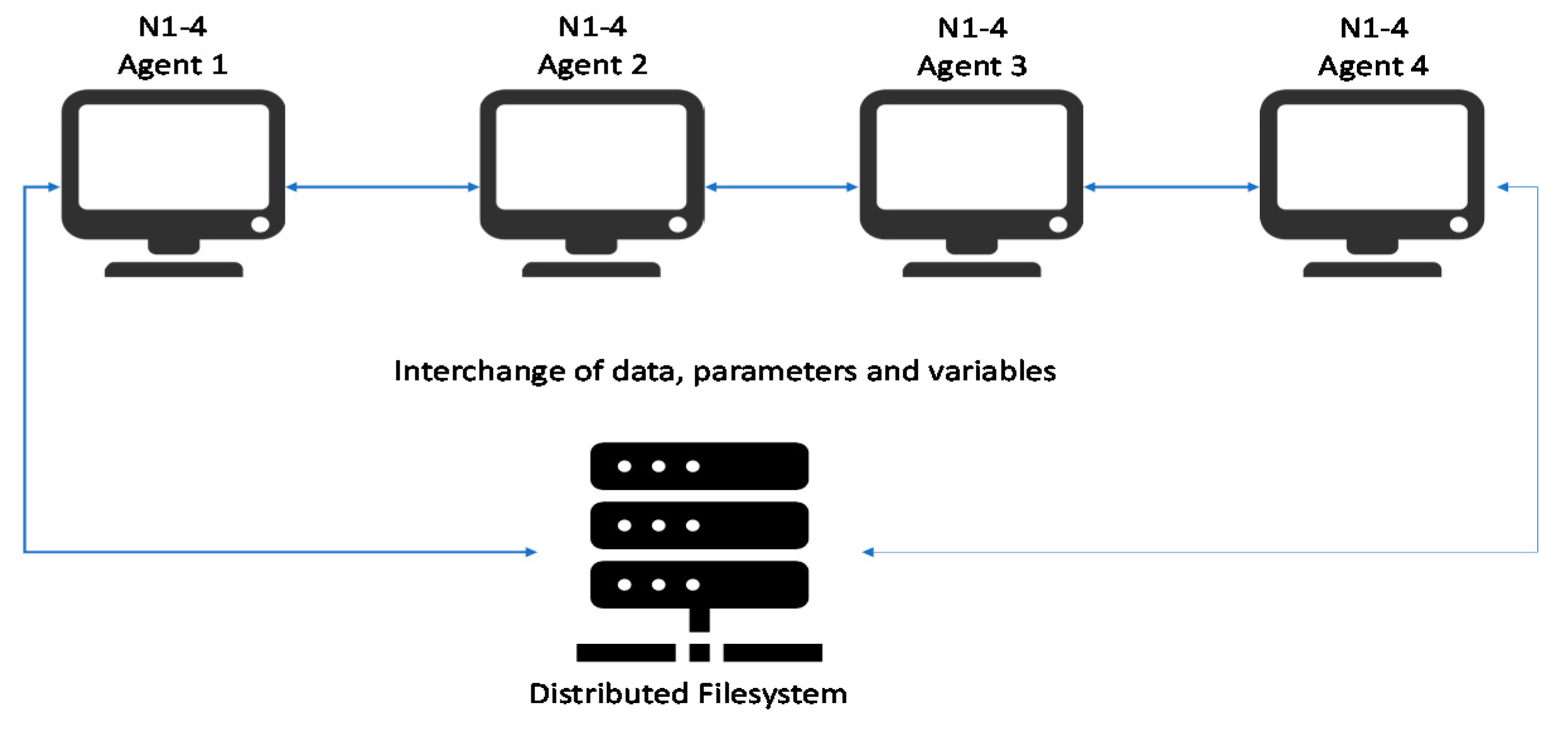
The platform used to execute preprocessing distributed functions was hosted on Google Cloud, selecting basic machines, named n1–4, which provide a four-core central processing unit (CPU) and 15 GB of random-access memory (RAM). The instances were connected between a shared file system based on network file system (NFS) to share the software components.

As can be seen in Figure 1, the machines need to be connected with each other, in order to be able to exchange data. Parameters and variables are executed just as if they were a single computer executing a program. Another important detail is the presence of a distributed filesystem; different machines must access the same filesystem to make sure they share the same input files.

Algorithm 1 Preprocessing UGR’16 dataset

1:preprocess_dataset.py 2: open full dataset file 3: drop incomplete rows 4: for every machine available: 5:      create one thread per CPU core 6: START OF DISTRIBUTED PREPROCESING FUNTION 7: while not processed features available do: 8: # Code executed in parallel at each machine 9:      for every free thread in parallel do: 10:          feature to preprocess = random feature from the dataset not processed yet 11:          process_piece(feature to preprocess): 12:              if feature is duration or number of packets or bytes: 13:                  code each value as normal distribution of all 14:              if feature is type of traffic: 15:                  code as type of traffic with int 16:              else: 17:                  assign each distinct value a number 18:          save column into final dataset 19:          Give result to machine one 20:      Continue 21: END OF DISTRIBUTED PREPROCESING FUNTION 22: continue 23: write final dataset into file

Algorithm 1 presents how the dataset is preprocessed. This task is done by columns because it is mandatory to consider the different values in each feature (each feature correspond with a column). This allows building an index array of the different elements, which is used to calculate the normal distribution of the values that shape the feature or just to encode them in the desired way as required in each case.

The whole process is done in an agile way, dividing the different functions correctly and protecting critical reading/writing operations to provide reliable operation of the software that will be executed in parallel in the above-mentioned machines.

One of the available threads (launched continuously) manages the execution. This first thread starts by opening the full dataset file and the different columns corresponding with each feature identified. Then, this first thread starts assigning features for preprocessing to each of the available threads (lines 6–18 in Algorithm 1) in parallel. Once the tasks finish, each thread returns the result to the first thread, which assigns more features in parallel until there are no more to process. Finally, the results are stored in a file that will be ready to be used by the corresponding machine learning algorithm.

5.3. Machine Learning Dataset Preprocessing

As mentioned before, there exist numerous ML algorithms. The most reliable algorithms for this task are multilayer perceptron (MLP) and decision trees (DT), as discussed in Reference [45]. For this reason, different solutions for both algorithms were tested and measured to get the best solution.

5.3.1. Multilayer Perceptron Processing

MLPs are feed-forward neural networks that consist of a large number of connected neurons divided into input units, output units, and hidden units. In general, MLP consists of a linear classifier able to sort the input data into two differentiated categories, by using a feature vector multiplied by some weights and added to a bias [46]. In this sense, the correct implementation of an MLP algorithm is performed by defining the following variables that will make up the underlying neural network:

• Number and type of features;
• Preprocessing of the chosen data associated with the features;
• Architecture of the neural network;
• Number of hidden layers and input nodes;
• Activation function;
• Loss function;
• Data validation.

The machines that process the algorithm use their graphics processing units (GPUs) and CPUs to increase its efficiency. The number and type of features and their preprocessing was addressed in Section 5.1. Additionally, in that same section, the architecture of the neural network was settled in 10 input values. The output was defined by a binary result, where 0 means no attack and 1 means attack. Between the input and output layer, two hidden layers were added. A hidden layer helps to represent different decisions that could not be directly related to the linear results of the features. The first layer helps to approximate functions that contain a continuous mapping from one finite space to another, and the second layer could represent an arbitrary decision boundary to arbitrary accuracy. For this reason, the neural network that is created has two hidden layers, this makes it capable of identifying arbitrary solutions.

In addition, some other important parameters that the neural network must have are the activation function and the kernel initializer function or the optimizer. In this case, the activation function selected was ReLU; this decision was made following the previous work carried out by the authors and presented in Reference [18], where a comparative analysis of different activation functions for MLP is shown.

Thus, the model proposed in this research was developed by using Keras (Alphabet Inc., Mountain View, CA, USA) and defined by four layers: one input layer, two hidden layers, and one output layer. The input layer was designed by including one node for each input feature. On the other hand, the number of hidden layers was determined using Equation (1), selected after evaluating the four previously proposed equations [18]. Furthermore, in every layer except in the output, the “softmax” function was used, as it facilitates the probability distribution among a different number of categories [47]. The kernel initializer function selected was the “normal” and the optimizer was implemented by an “adam” optimizer [48,49]. EarlyStopping [50] was used in the proposed model in order to prevent the overfitting with a min_delta of 10⁻³, which is the minimum value of the loss in order to determine an improvement of the number of epochs in the model.

5.3.2. Decision Tree Processing

A decision tree is a flowchart tree structure. It is characterized by internal nodes, one for each variable that makes up the input dataset. From them, new branches appear, each of which represents a decision rule. At the end of the tree, each leaf-node represents an outcome, the result of the calculation. In addition, unlike neural networks, which are black boxes, in a decision tree, the calculations being made are easy to understand because it is totally transparent [51].

Decision trees follow some specific steps to build the most effective tree to get the best results in each case. That is, it looks for the best feature of the dataset using an algorithm called “attribute selection measures” to split the dataset into different parts, i.e., smaller subsets. This process is repeated recursively for each new child, trying to meet one of the desired conditions. The possible stop conditions are the lack of attributes, the lack of subsets, or the leaves that last belonging to the same attribute [51]. As can be seen, the attribute selection measure is the cornerstone of the decision trees. The main idea behind it is to provide each feature with a rank by explaining the input dataset. The one with the best rank is selected as the splitting feature.

There are different algorithms to determine the rank. The most common one is the “information gain” which calculates the entropy of the features that shape the dataset in order to measure the “randomness” of the set. Furthermore, the entropy and “Gini index” are used to measure a weighted sum of the impurity of each partition of the selected features [52]. Different tests were carried out in order to reach different results. Some other parameters that can be chosen in a decision tree are the depth of the tree itself, to make simpler trees that are not overfitted, or the criteria to split the dataset itself (not the feature), by choosing the best split calculated or by randomizing the process.

6. Validation

6.1. Dataset Processing

In order to evaluate the performance of the developed system, some timing comparisons were made between the originally developed script and the one created with the new algorithm proposed for distributed preprocessing, while also including different dataset sizes.

The tests related to a single machine were run in one of the machines that shaped the new algorithm proposed for distributed preprocessing circle. The shared filesystem for the new algorithm proposed for distributed preprocessing was based on NFS as described in Section 5.2.

With this infrastructure, the different tests could be easily performed. The achieved results are summarized in

Table 3. Comparison of the time it takes to process the dataset with distributed preprocessing or locally for different sizes (in lines) of the dataset.

Size(.tar) Compressed	Dataset Size (Lines)	Execution Time Locally (s)	Execution Time in Distributed Preprocessing (s)
9.2 MB	100,000	5.67	4.25
~99 MB	1,000,000	51.82	25.52
~495 MB	5,000,000	257.06	139.70
~1 GB	10,000,000	529.09	300.96
~5 GB	50,000,000	2737.52	1363.32
~14.56 GB	157,602,189	13,846.43	6451.53

where the time is measured in seconds and the dataset size is shown in lines. Here, 100,000 lines are equivalent to nearly 9.2 MB in compressed format.

The results show that the distributed preprocessing architecture achieved significantly better results than execution in a single machine thanks to the parallelization of tasks. The developed algorithm makes it easier to open large datasets for preprocessing purposes in machines that do not have many resources to be used, while the distributed preprocessing architecture makes the execution run in less time, reducing costs.

In conclusion, the distributed preprocessing architecture reduces the time costs of the dataset preprocessing, one of the most important problems when dealing with big datasets. A large dataset containing more than 157,602,189 traffic flows, of which 2,324,955 are attacks, collected during July 2016 [24], with a size of more than 15 GB in compressed format, can be processed in a manageable amount of time using our distributed architecture proposal. For this reason, in the following sections, this dataset is the one chosen to train the neural network and the decision tree as it contains a huge amount of information and different types of attacks.

Table 4. Relation between the type of attacks and the number of their appearances in the preprocessed dataset.

Type of Attacks	Appearances
No attack	155,277,234
Denial of Service	783,253
Spam	491,487
Network Scan	449,406
Blacklisted	449,381
Botnet	151,428

summarizes different attacks classified within the dataset presented in the preprocessed UGR’16 [24].

6.2. Evaluation of Multilayer Perceptron Neural Network

Once the model is obtained and the large-scale dataset is preprocessed, the objective is to develop an IDS with high capacities. Since the idea is to achieve the process in the most optimized way possible, a series of additional tools were used to improve the performance.

The first of these measures was applied because Google Cloud (Alphabet Inc., Mountain View, CA, USA) instances use a modern Intel (Intel Corp., Santa Clara, CA, USA) architecture. Intel developed a compiled version optimized for the most advanced instructions of its latest processors.

However, as explained below, the desired architecture turned out to be unfeasible, because the memory required by the neural network itself made it almost impossible to scale.

The different experiments consisted of using different architectures in order to fulfill the requirements of the model proposed. These tests were performed by scaling the architecture characteristics as necessary by adding more CPU cores, more memory, and even different GPUs. These results show that the different computational architecture configurations tested prevent the proposed ML model from being executed, either due to errors (ResourceExhaustedError, MemoryError) or due to inefficient computation time (400,000 h per epoch), as presented in

Table 5. Evaluation of neural networks with the multilayer perceptron (MLP) algorithm. CPU—central processing unit; GPU—graphics processing unit.

CPUs	Memory	GPUs	Result
8 cores	32 GB	None	MemoryError
16 cores	64 GB	None	ResourceExhaustedError
32 cores	100 GB	None	ResourceExhaustedError
32 cores	200 GB	None	400,000 h per epoch
16 cores	32 GB	×1 Tesla K80 (12 GB)	MemoryError
32 cores	64 GB	×2 Tesla K80 (24 GB)	ResourceExhaustedError
32 cores	100 GB	×4 Tesla K80 (48 GB)	ResourceExhaustedError
32 cores	200 GB	×8 Tesla K80 (96 GB)	ResourceExhaustedError

.

In conclusion, the MLP neural networks cannot be trained this way with large datasets. The limitations of this architecture make it not scalable and, therefore, impossible to train a model in an assumable amount of time. In addition, training it using multiple GPUs, despite being theoretically faster, is limited by the size of the model itself, which, regardless of the number of graphics processor units used, must be able to be stored completely in the memory of each of them in order to perform the training. Furthermore, regarding GPU training, when the training process takes place on multiple GPUs, as explained above, the CPU is responsible for creating the model, processing the batches, and assigning them to each GPU. In this process, an overhead is added. Although that overhead is negligible in small models, it becomes more and more noticeable in large neural networks, increasing the training time with respect to training in a CPU with many cores, or even making this training impossible because of the size achieved. This additional overhead is fixed since it serves to relocate the output information of the training in the final model that the CPU itself is building.

6.3. Evaluation of Decision Trees

The test for the different types of decision trees was carried out by using different types of attribute selection measures and different features split approaches. To develop the different tests, the architecture used was based on an instance in Google Cloud. Considering the size of the dataset, the needed memory for the instance to develop its activity must be enough to include the dataset itself and the model to train with it. For this reason, the initially chosen machine contained 100 GB of RAM memory and an eight-core processor. Four different combinations were tested. Three parameters were measured: the time needed to carry out the training, the precision, and the error, all of which are detailed in

Table 6. Summary of the result achieved using different combinations of algorithms for decision trees using the fully preprocessed dataset.

		Quality of Split
		“Gini”			“Entropy”
		Time	Accuracy	Error	Time	Accuracy	Error
Splitter strategy	Best	2899.448	0.999	0.0012	3423.31	0.999	0.0011
	Random	497.19	0.989	0.0120	448.976	0.988	0.0119

.

When the random splitting criteria are applied, the time needed to make the calculations is heavily reduced, since it does not calculate which one is better, choosing one random feature to continue the tree. This is penalized by reducing the accuracy and lightly elevating the error rate, which is, however, almost negligible.

More important than accuracy and times for training are the threat detection rates, since the IDS is expected to detect as many security problems as possible. Given the available attacks that were present in the preprocessed dataset and summarized in Table 4, confusion matrices were obtained for each of the cases.

The first important conclusion from the results is that the random splitting strategy is not a valid solution. An IDS cannot have such a high false negative rate, detecting 72.33% of the cases as “no attack” when it really was an attack in the worst case. This rate was lowered to 6.33% of the false negative rate in the entropy/best combination, which can be classified as acceptable, since, with an IDS, it is preferable to have a higher rate of false positives rather than false negatives.

In each case, the decision tree was generated so that the criteria followed by the algorithm could be checked. Thanks to this, it was possible to verify that the main criteria that the decision tree took were the origin and destination IP addresses.

These IP addresses, coded as an index, were only an anonymized number since this was done in the dataset itself. It is logical to think that data such as the port of origin and destination, the duration of the flow, or the amount of data transmitted are more important. For this reason, it was decided to repeat the test, this time removing the trace of IP addresses from the dataset. In this repetition, the best results balancing quality and time were again achieved with the “entropy” calculation and “best” splitting strategy. The time needed to execute this algorithm was 2786.77 seconds. The accuracy achieved was 0.99614035. Logically, the amount of time needed decreased, while the distribution of accuracy and error remained the same. The confusion matrix for this case is presented in

Table 7. Confusion matrix of multi attack classification.

True Label/ Predicted Label	DoS	Net Scan	Botnet	Blacklist	Spam	No Attack
DoS	235,635	0	0	0	0	64
Net Scan	0	133,500	0	0	0	1424
Botnet	0	0	16,601	0	0	28,726
Blacklist	10	4	0	1358	7	133,319
No Attack	0	0	0	0	140,379	7526

.

In this case, the false negative rate increased slightly, with a 24% rate. However, looking at the decision tree, it is more logical to think that this algorithm is more prepared to predict attacks in more situations since it is not using IP addresses.

Furthermore, analyzing how the model is predicting attacks, several conclusions can be drawn. Firstly, the model presents good results in the classification of network denial of service attacks, with a success rate of 99.97%. Similar cases occur with network scans and spam detection, with 98.94% and 94.91%, respectively. On the other hand, the model did not find a good relationship between information in traffic flows and botnets since its success rate was only 36.62%. The model cannot predict blacklisted traffic, with a success rate of only 1%. These results are summarized in

Table 8. Results achieved with the decision tree algorithm.

	DoS	Net Scan	Botnet	Blacklist	Spam	No attack
Accuracy	99.97%	98.94%	36.62%	1.01%	94.91%	99.98%

.

The achieved results were good, and the IDS is expected to perform adequately. The worst rates, achieved in the predictions of blacklisted traffic, are not a real problem since there are good alternative methods to detect this kind of attacks [53], e.g., based on blacklist malicious IPs formed by different feeds obtained from malicious IP service providers.

7. Discussion

Due to the enormous amount of information needed to determine an attack, limiting information contained by cybersecurity datasets stands as an issue for developing detection systems. Consequently, the information offered by this kind of datasets should be reduced to the most useful to feed the underlying ML algorithms. For this reason, UGR’16 was selected as a basis dataset in this research, a dataset that contains information strongly focused on attack detection within real ISP network traffic.

As mentioned throughout this article, to achieve a successful result in detecting attacks and intrusions by means of an IDS based on AI, a thorough training of the underlying ML model is necessary. For this process, trying to use as much as information as possible offered by the dataset is important to achieve good results.

The time invested in this preprocessing remained below 6500 seconds, a fact that meets the expectations and objectives defined previously. Table 3 shows the results given by parallelism and local execution, and it leads to the fact that that its comparison in terms of complexity is not parallel. This is because the time required for the processing of the individual functions is related to the feature preprocessing encoding in each machine. The model, therefore, demonstrated a correct level of scalability while maintaining a balance among costs, execution time, and the specific knowledge required for its execution.

The second objective of this research was focused on the training process of an ML model, using for this the full portion of the preprocessed data. This process was approached from two perspectives, using MLP neural networks with different configurations, and through decision trees.

Table 9. Comparison between MLP and decision trees.

	CPU	GPU	Memory	Time	Result
MLP	32 cores	None	200 GB	400,000 h per epoch	None
DT	8 cores	None	50 GB	3500 seconds	99.61%

shows a comparison between both approaches.

For the first approximation, the results show problems related to its scalability and the consumption of computational resources. The DL model implemented required a memory space greater than five times the size of the data subset, that is, 120 GB. The training based on CPUs, despite being slow and requiring hundreds of thousands of hours to process each epoch, is possible. TensorFlow is able to scale the model to make use of all the available cores in the CPU. However, it is not optimal due to the number of hours needed. By using GPUs, it is possible to obtain better results in terms of time due to the use of several GPUs at the same time. However, to perform training on several GPUs at once, it is necessary to add an overhead of data to the batches that, in each epoch, are sent to each GPU to relocate the results to the complete original model. This makes large models a much slower process due to the large overhead added. To avoid scalability problems, the library of python for machine learning applications, Keras [54], uses TensorFlow (2.0, Santa Clara, CA, USA) [55], providing a method to perform the training by using a Python generator that collects small portions of the original dataset. However, the UGR’16 dataset contains more background traffic than any other kind and, therefore, the most probable event is that the portions on which the algorithm is trained only contain background traffic, without attacks. Therefore, the model will generate false negatives. Thus, we can conclude that this kind of architecture is not ready for training MLP networks by use of large datasets, because, despite using very powerful machines with multiple CPUs, GPUs, and large amounts of memory, the cost of training remains very high, as shown in Table 4.

In contrast to this first approach, the same tests were attempted on a simpler algorithm such as the decision tree. For this method, a comparison was made of all the algorithms used to calculate the decision tree. The results obtained led to several conclusions. By using this kind of algorithm, it was possible to obtain results with machines with more limited resources and less time. In the worst case, the construction of the entire decision tree using the preprocessed dataset took less than 3500 s. Analyzing the decision tree created from the training, we observed how the IP addresses, both origin and destination, were taken as a key variable, something that led to unacceptable results. This was due to IP addresses being easily changeable data for most attacks. Therefore, we decided not to consider those data during the training. By adapting the training in this way, we obtained results that show that decision trees achieved a good overall precision. More specifically, the results of the model were successful in obtaining a classification network for denial of service attacks, with a success rate of 99.97%. Similar results were achieved when detecting network scans and spam, with 98.94% and 94.91%, respectively. The accuracy of the results was reduced when predicting botnet attacks (36.62%) and especially when predicting blacklist traffic (1%). In general, the results are faster and more reliable compared with neural networks.

As stated in Section 2, there are different approaches for classification for IDSs based on anomaly detection.

Table 10. Comparison between proposed solution and related works.

	Scalable	Best Algorithm	Accuracy BC	Accuracy Multi-Class Classification					Large Scale	Training Time (s)	Gb Data
				DoS	NetScan	Botnet	Blacklist	Spam	Dataset
Proposed solution	✓	DT	99.61	99.27	98.24	98.94	1.01	94.91	✓ (UGR16)	3500	~14 GB (compressed)
[5]	X	DT	X	97.24	97.24	77.92	X	X	X (KDD’99)	X	~0.5 GB
[7]	✓	DT	91.64	X	X	X	X	X	X (NSL-KDD)	344	~0.5 GB
[22]	✓	DT	97.49	X	X	X	X	X	X (UNSW-NB15)	5.69	~0.5 GB
[22]	✓	SVM	92.28	X	X	X	X	X	X (UNSW-NB15)	38.91	~0.5 GB
[18]	X	NN (MLP)	99	X	X	X	X	X	X (UNSW-NB15)	X	~0.5 GB

compares the model proposed in this paper with some of those included in the literature, based on different aspects such as multi-class classification, binary classification (BC), training time, model proposed, scalability of the software, and quantity of data analyzed.

Despite all the efforts made in this area of research, most of the existing approaches do not analyze truly large-scale datasets as proposed in this paper. Our solution demonstrated that it is able to train up to 14 GB of data (compressed) detecting new and reliable modern attacks with high accuracy using the benchmark dataset UGR’16.

8. Conclusions and Future Directions

Due to the enormous amount of information needed to determine an attack and the problems with processing and preprocessing large-scale datasets, as outlined in this article, it is necessary to use up-to-date, real sensor-based traffic datasets. That is why, in this work, we proposed the use of the new dataset UGR16, which contains a large amount of real traffic collected from network sensors in two ISPs.

Taking into account the first objective of this research, using the model presented in Section 5.2, it was possible to use a great portion of the dataset while reducing the time taken to preprocess the data by more than 50% when compared with its local execution. The second objective of this research was focused on the training process of an ML model, using the full preprocessed data. This process was approached from two perspectives, using MLP neural networks, and through decision trees. Using an MLP neural network required a high amount of memory in order to train the preprocessed data. That memory can be up to five times the size of the dataset. The CPU can process this huge amount of data despite the high time needed to process it. Instead, by using GPUs, it is possible to obtain better results in terms of time due to the use of several GPUs at the same time. However, to perform training on several GPUs at once, it is necessary to add an overhead of data to the batches that, in each epoch, are sent to each GPU to relocate the results to the complete original model. This slows down the process due to the large overhead added.

In contrast to this first approach, the same tests were attempted on a simpler algorithm such as the decision tree. For this method, a comparison was made of all the algorithms used to calculate the decision tree. The training time was lower versus the MLP algorithm, and the precision obtained demonstrated success per type of attack with rates over 99% in denial of service, spam detection, and scan detection. Instead, the detection of botnet attacks achieved a lower accuracy. Blacklist traffic, as mentioned above, can be identified with feeds for blacklist IP servers in this case.

Additionally, this research provides new information related to preprocessing and processing information within applications to machine learning algorithms for large-scale sensor-based datasets. As future lines of research, there could be an approach to implement the proposed architecture with more complex tools such as Apache Spark which might show the benefit of our work due to its approach to distributed systems. Moreover, it would be interesting to explore new alternatives to preprocess the data in systems like HPC (high-performance computing) in order to reduce the complexity when dealing with big files to be preprocessed. Furthermore, in this research, we found that a deep learning algorithm such as MLP is not suitable for large-scale datasets; thus, it would be necessary to improve the algorithm being applied to distributed systems using distributed libraries developed for Apache Spark.

References

- Key Challenges. Available online: https://www.weforum.org/centre-for-cybersecurity/home/ (accessed on 15 April 2019).
- Geluvaraj, B.; Satwik, P.M.; Kumar, T.A. The Future of Cybersecurity: Major Role of Artificial Intelligence, Machine Learning, and Deep Learning in Cyberspace. In Proceedings of the International Conference on Computer Networks and Communication Technologies; Springer: Singapore, 2019; pp. 739–747. [Google Scholar]
- Tjhai, G.C.; Papadaki, M.; Furnell, S.M.; Clarke, N.L. Investigating the problem of IDS false alarms: An experimental study using Snort. In Proceedings of the Ifip Tc 11 23rd International Information Security Conference; Jajodia, S., Samarati, P., Cimato, S., Eds.; Springer: Boston, MA, USA, 2008; Volume 278, pp. 253–267. ISBN 978-0-387-09698-8. [Google Scholar]
- Hu, L.; Li, T.; Xie, N.; Hu, J. False positive elimination in intrusion detection based on clustering. In Proceedings of the 2015 12th International Conference on Fuzzy Systems and Knowledge Discovery (FSKD), Zhangjiajie, China, 15–17 August 2015; pp. 519–523. [Google Scholar]
- Mishra, P.; Varadharajan, V.; Tupakula, U.; Pilli, E.S. A Detailed Investigation and Analysis of Using Machine Learning Techniques for Intrusion Detection. IEEE Commun. Surv. Tutor. 2019, 21, 686–728. [Google Scholar] [CrossRef]
- Tavallaee, M.; Bagheri, E.; Lu, W.; Ghorbani, A.A. A detailed analysis of the KDD CUP 99 data set. In Proceedings of the 2009 IEEE Symposium on Computational Intelligence for Security and Defense Applications, Ottawa, ON, Canada, 8–10 July 2009; pp. 1–6. [Google Scholar]
- Gupta, G.P.; Kulariya, M. A Framework for Fast and Efficient Cyber Security Network Intrusion Detection Using Apache Spark. Procedia Comput. Sci. 2016, 93, 824–831. [Google Scholar] [CrossRef] [Green Version]
- Flow-Based Intrusion Detection: Techniques and Challenges | Elsevier Enhanced Reader. Available online: https://reader.elsevier.com/reader/sd/pii/S0167404817301165?token=E3C74A2C564F117F985E7ED42B8710D395BFDF2BA31F99DBA65E63B3295E5B3D75000B3FC3E01132C2E06A2ACDE52A92 (accessed on 20 June 2019).
- Strigl, D.; Kofler, K.; Podlipnig, S. Performance and Scalability of GPU-Based Convolutional Neural Networks. In Proceedings of the 2010 18th Euromicro Conference on Parallel, Distributed and Network-based Processing; IEEE: Piscataway, NJ, USA, 2010; pp. 317–324. [Google Scholar]
- Maciá-Fernández, G.; Camacho, J.; Magán-Carrión, R.; García-Teodoro, P.; Therón, R. UGR‘16: A new dataset for the evaluation of cyclostationarity-based network IDSs. Comput. Secur. 2018, 73, 411–424. [Google Scholar] [CrossRef] [Green Version]
- Hindy, H.; Brosset, D.; Bayne, E.; Seeam, A.; Tachtatzis, C.; Atkinson, R.; Bellekens, X. A Taxonomy and Survey of Intrusion Detection System Design Techniques, Network Threats and Datasets. arXiv 2018, arXiv:1806.03517 [cs]. [Google Scholar]
- MIT Lincoln Laboratory: DARPA Intrusion Detection Evaluation. Available online: https://www.ll.mit.edu/ideval/data/ (accessed on 22 May 2018).
- Perona, I.; Arbelaiz Gallego, O.; Gurrutxaga, I.; Martín, J.I.; Muguerza Rivero, J.F.; Pérez, J.M. Generation of the database gurekddcup. 2017. Available online: https://addi.ehu.es/handle/10810/20608 (accessed on 15 May 2020).
- Shiravi, A.; Shiravi, H.; Tavallaee, M.; Ghorbani, A.A. Toward developing a systematic approach to generate benchmark datasets for intrusion detection. Comput. Secur. 2012, 31, 357–374. [Google Scholar] [CrossRef]
- Analysis, C.C.; For A.I.D. CAIDA: Center for Applied Internet Data Analysis. Available online: http://www.caida.org/home/index.xml (accessed on 11 September 2019).
- Revathi, S.; Malathi, D.A. A Detailed Analysis on NSL-KDD Dataset Using Various Machine Learning Techniques for Intrusion Detection. Int. J. Eng. Res. Technol. 2013, 2, 1848–1853. [Google Scholar]
- Alrawashdeh, K.; Purdy, C. Toward an online anomaly intrusion detection system based on deep learning. In Proceedings of the 2016 15th IEEE International Conference on Machine Learning and Applications (ICMLA), Anaheim, CA, USA, 18–20 December 2016; pp. 195–200. [Google Scholar]
- Larriva-Novo, X.A.; Vega-Barbas, M.; Villagra, V.A.; Sanz Rodrigo, M. Evaluation of Cybersecurity Data Set Characteristics for Their Applicability to Neural Networks Algorithms Detecting Cybersecurity Anomalies. IEEE Access 2020, 8, 9005–9014. [Google Scholar] [CrossRef]
- Shahamiri, S.R.; Binti Salim, S.S. Real-time frequency-based noise-robust Automatic Speech Recognition using Multi-Nets Artificial Neural Networks: A multi-views multi-learners approach. Neurocomputing 2014, 129, 199–207. [Google Scholar] [CrossRef]
- Gaidhane, R.; Vaidya, C.; Raghuwanshi, D.M. Intrusion Detection and Attack Classification using Back-propagation Neural Network. Int. J. Eng. Res. 2014, 3, 4. [Google Scholar]
- Karsoliya, S. Approximating Number of Hidden layer neurons in Multiple Hidden Layer BPNN Architecture. Int. J. Eng. Trends Technol. 2012, 3, 714–717. [Google Scholar]
- Belouch, M.; El Hadaj, S.; Idhammad, M. Performance evaluation of intrusion detection based on machine learning using Apache Spark. Procedia Comput. Sci. 2018, 127, 1–6. [Google Scholar] [CrossRef]
- Tu, D.Q.; Kayes, A.S.M.; Rahayu, W.; Nguyen, K. ISDI: A New Window-Based Framework for Integrating IoT Streaming Data from Multiple Sources. In Proceedings of the Advanced Information Networking and Applications; Barolli, L., Takizawa, M., Xhafa, F., Enokido, T., Eds.; Springer International Publishing: Cham, Switzerland, 2020; pp. 498–511. [Google Scholar]
- Rajagopal, S.; Kundapur, P.P.; Hareesha, K.S. A Stacking Ensemble for Network Intrusion Detection Using Heterogeneous Datasets. Secur. Commun. Netw. 2020, 2020, 4586875. [Google Scholar] [CrossRef] [Green Version]
- Learning, D. Ian Goodfellow, Yoshua Bengio, Aaron Courville; MIT Press: Cambridge, MA, USA, 2016. [Google Scholar]
- Brownlee, J. Supervised and unsupervised machine learning algorithms. Mach. Learn. Mastery 2016, 16. [Google Scholar]
- Gardner, M.W.; Dorling, S.R. Artificial neural networks (the multilayer perceptron)—A review of applications in the atmospheric sciences. Atmos. Environ. 1998, 32, 2627–2636. [Google Scholar] [CrossRef]
- Heaton, J. AIFH, Volume 3: Deep Learning and Neural Networks; Heaton Research, Inc, 2015; ISBN 1-5057-1434-6. [Google Scholar]
- Vinayakumar, R.; Soman, K.P.; Poornachandran, P. Applying convolutional neural network for network intrusion detection. In Proceedings of the 2017 International Conference on Advances in Computing, Communications and Informatics (ICACCI), Udupi, India, 13–16 September 2017; pp. 1222–1228. [Google Scholar]
- Haykin, S. Neural Networks: A Comprehensive Foundation, 1st ed.; Prentice Hall PTR: Upper Saddle River, NJ, USA, 1994; ISBN 978-0-02-352761-6. [Google Scholar]
- Saha, S. A Comprehensive Guide to Convolutional Neural Networks—The ELI5 Way. Available online: https://towardsdatascience.com/a-comprehensive-guide-to-convolutional-neural-networks-the-eli5-way-3bd2b1164a53 (accessed on 20 June 2019).
- Krizhevsky, A.; Sutskever, I.; Hinton, G.E. ImageNet Classification with Deep Convolutional Neural Networks. In Advances in Neural Information Processing Systems 25; Pereira, F., Burges, C.J.C., Bottou, L., Weinberger, K.Q., Eds.; Curran Associates, Inc.: Red Hook, NY, USA, 2012; pp. 1097–1105. [Google Scholar]
- Breiman, L. Classification and Regression Trees; Routledge: London, UK, 2017; ISBN 978-1-315-13947-0. [Google Scholar]
- Liberman, N. Decision Trees and Random Forests. Available online: https://towardsdatascience.com/decision-trees-and-random-forests-df0c3123f991 (accessed on 20 June 2019).
- Wang, F.; Wang, Q.; Nie, F.; Yu, W.; Wang, R. Efficient tree classifiers for large scale datasets. Neurocomputing 2018, 284, 70–79. [Google Scholar] [CrossRef]
- Peng, K.; Leung, V.C.M.; Zheng, L.; Wang, S.; Huang, C.; Lin, T. Intrusion Detection System Based on Decision Tree over Big Data in Fog Environment. Available online: https://www.hindawi.com/journals/wcmc/2018/4680867/abs/ (accessed on 21 November 2019).
- Gupta, P. Decision Trees in Machine Learning. Available online: https://towardsdatascience.com/decision-trees-in-machine-learning-641b9c4e8052 (accessed on 20 June 2019).
- Decision Tree Classification in Python. Available online: https://www.datacamp.com/community/tutorials/decision-tree-classification-python (accessed on 31 May 2019).
- Breiman, L. Random Forests. Mach. Learn. 2001, 45, 5–32. [Google Scholar] [CrossRef] [Green Version]
- Nearest Neighbor Pattern Classification. Available online: https://scholar.googleusercontent.com/scholar?q=cache:0XrqZfG45o0J:scholar.google.com/+k+nearest+neighbor&hl=es&as_sdt=0,5&as_vis=1 (accessed on 20 June 2019).
- Gandhi, R. K Nearest Neighbours—Introduction to Machine Learning Algorithms. Available online: https://towardsdatascience.com/k-nearest-neighbours-introduction-to-machine-learning-algorithms-18e7ce3d802a (accessed on 20 June 2019).
- Aldweesh, A.; Derhab, A.; Emam, A.Z. Deep learning approaches for anomaly-based intrusion detection systems: A survey, taxonomy, and open issues. Knowl. Based Syst. 2020, 189, 105124. [Google Scholar] [CrossRef]
- Moradi, M.; Zulkernine, M. A Neural Network Based System for Intrusion Detection and Classification of Attacks. In Proceedings of the IEEE International Conference on Advances in Intelligent Systems-Theory and Applications, Luxembourg-Kirchberg, Luxembourg, 15–18 November 2004. [Google Scholar]
- Jalberca. Anomaly-based Intrussion Detection System with machine learning and distributed execution. Available online: https://github.com/jalberca/tfm-ids_and_machine_learning (accessed on 13 May 2020).
- Soysal, M.; Schmidt, E.G. Machine learning algorithms for accurate flow-based network traffic classification: Evaluation and comparison. Perform. Eval. 2010, 67, 451–467. [Google Scholar] [CrossRef]
- Chiba, Z.; Abghour, N.; Moussaid, K.; El Omri, A.; Rida, M. A novel architecture combined with optimal parameters for back propagation neural networks applied to anomaly network intrusion detection. Comput. Secur. 2018, 75, 36–58. [Google Scholar] [CrossRef]
- Ramachandran, P.; Zoph, B.; Le, Q.V. Searching for Activation Functions. arXiv 2017, arXiv:1710.05941. [Google Scholar]
- Brownlee, J. Gentle Introduction to the Adam Optimization Algorithm for Deep Learning. Machine Learning Mastery. Available online: https://machinelearningmastery.com/adam-optimization-algorithm-for-deep-learning/ (accessed on 13 May 2020).
- Kingma, D.P.; Ba, J. Adam: A Method for Stochastic Optimization. arXiv 2014, arXiv:1412.6980 [cs]. [Google Scholar]
- Callbacks-Keras Documentation. Available online: https://keras.io/callbacks/#earlystopping (accessed on 21 November 2019).
- Bouzida, Y.; Cuppens, F. Neural networks vs. decision trees for intrusion detection. In Proceedings of the IEEE/IST workshop on monitoring, attack detection and mitigation (MonAM), Citeseer, Tuebingen, September 2006; 28, p. 29. [Google Scholar]
- White, A.P.; Liu, W.Z. Bias in information-based measures in decision tree induction. Mach. Learn. 1994, 15, 321–329. [Google Scholar] [CrossRef]
- Ghafir, I.; Prenosil, V. Blacklist-based malicious IP traffic detection. In Proceedings of the 2015 Global Conference on Communication Technologies (GCCT), Thuckalay, India, 23–24 April 2015; pp. 229–233. [Google Scholar]
- Keras Documentation. Available online: https://keras.io/ (accessed on 4 June 2018).
- TensorFlow. Available online: https://www.tensorflow.org/?hl=es (accessed on 14 June 2019).
© 2020 by the authors. Licensee MDPI, Basel, Switzerland. This article is an open access article distributed under the terms and conditions of the Creative Commons Attribution (CC BY) license (http://creativecommons.org/licenses/by/4.0/).