Numerical Investigation into the Effect of Different Parameters on the Geometrical Precision in the Laser-Based Powder Bed Fusion Process Chain

Abstract

Due to the layer-by-layer nature of the process, parts produced by laser-based powder bed fusion (LPBF) have high residual stresses, causing excessive deformations. To avoid this, parts are often post-processed by subjecting them to specially designed heat treatment cycles before or after their removal from the base plate. In order to investigate the effects of the choice of post-processing steps, in this work the entire LPBF process chain is modelled in a commercial software package. The developed model illustrates the possibilities of implementing and tailoring the process chain model for metal additive manufacturing using a general purpose finite element (FE) solver. The provided simplified computational example presents an idealised model to analyse the validity of implementing the LPBF process chain in FE software. The model is used to evaluate the effect of the order of the process chain, the heat treatment temperature and the duration of the heat treatment. The results show that the model is capable of qualitatively capturing the effect of the stress relaxation that occurs during a heat treatment at elevated temperature. Due to its implementation, the model is relatively insensitive to duration and heat treatment temperature, at least as long as it is above the relaxation temperature. Furthermore, the simulations suggest that, when post-processing, it is necessary to perform the stress relaxation before the part is removed from the base plate, in order to avoid a significant increase of the deformation. The paper demonstrates the capability of the simulation tool to evaluate the effects of variations in the process chain steps and highlights its potential usage in directing decision-making for LPBF process chain design.

1. Introduction

Additive manufacturing (AM) allows the manufacturing of parts with high complexity. Additionally, relatively short lead times, near-net-shape production and low material waste contribute to the increasing interest in AM. Focussing on AM of metals, laser-based powder bed fusion (LPBF) currently represents the industrially most relevant process [1], but some challenges remain for tooling steels [2], for example, residual stress build-up and the need for post-processing. LPBF, sometimes called selective laser melting, starts by depositing a thin layer of powder on a solid base plate. The laser melts the powder layer in the positions corresponding to a cross-section of a slice of the desired part. The machine then lowers the build plate with an amount corresponding to the thickness of the powder layer, and the process repeats until the part is completed.

Parts produced by LPBF are subjected to different stresses [3] during the production process due to this layer-by-layer method. Before the part is released from the build plate, the stresses in the top layer are typically tensile, while the bottom layer is subjected to compressive stress [4,5,6]. When the part is cut from the base plate, the release of these stresses leads to excessive deformation [5,6,7,8]. Avoiding or reducing this deformation is possible by applying a stress relief heat treatment [9]. In this post-process, the part is placed in a furnace, and due to the increase in temperature, the highest stresses in the part are reduced [10]. As a result of this stress relief heat treatment, the part will deform less when the residual stresses are released upon cutting from the build plate.

Additional heat treatment steps are often required, such as aging for optimal material properties, due to the thermal dependent nature of precipitation in some of the materials used in LPBF [11]. One of these materials, namely 17-4 precipitation hardening (PH) stainless steel [12], is the subject of the current paper. Alternatively, the part can be solution treated, to homogenise the microstructure, before the aging heat treatment takes place.

Prediction of the final deformations of a part produced by AM is important due to the strict tolerance requirements from industrial end users. A commonly used approach for satisfying these restrictions is using pre-deformation, meaning that the part is deformed in the opposite direction to the resultant from the AM process. After the part is cut from the base plate, the part deforms into the desired final shape. This approach is illustrated in the work by Yaghi et al. [13].

Although this method will result in functioning parts, it does not tackle the root issue of the process, namely the relation between the process parameters, the applied post-processing, and the final deformations. For example, changing the design of the part, or any of the process parameters, will result in a change in deformation and require a new compensational pre-deformation. The present work will implement a process chain model, which will provide insight into the effects of different process settings on the aforementioned deflections, therefore allowing the design of the process and post-process to prevent these deflections in the first place.

There are several numerical studies implementing such a process model. Focussing on single track simulations allows detailed investigation of all the different mechanisms taking place, due to the smaller simulation domain. Examples of such single track studies are the work by Antony et al. [14] and Bayat et al. [15]. Multi-track, or even multi-layer, models attempt to scale these detailed simulations up to more than one track, at the expense of high computational cost [16,17,18,19]. However, the current study focusses more on reduced fidelity numerical models, which allow the simulation of an entire AM process chain within a limited time. There are different approaches to obtain this fidelity reduction. Chen et al. [20] investigated the effect of the scanning strategy on the residual stresses by resolving the laser beam in a single layer with an exposed area of 4 mm². The number of elements required for this study was high, due to the large expected cooling rate and laser spot size. Denlinger [21] used a dynamic mesh coarsening algorithm. The mesh is fine where the laser surface heat flux interacts with the part and coarser in previously built layers, which effectively smears out the temperature and stress field in these layers. This strategy results in a high resolution simulation of a single cuboid, both thermally and mechanically. Similarly, Parry et al. [22] investigated the effect of scanning strategy and geometry of the part on the final deformations. Since they need to investigate the effect of the scanning direction, the laser itself needs to be resolved. This necessitates the choice of a fine mesh and therefore a small computational domain. Bayat et al. [23] simplified the laser by bunching the real layers together in so-called meta-layers and applying flash heating—the top of the meta-layer was exposed to an aggregated heat flux. Yakout et al. [24] investigated the effect of the thermal expansion coefficient and the thermal diffusivity on the residual stress after the LPBF. To achieve this, they simulated different materials and validated the model for one of them. They show that a low thermal coefficient and high thermal diffusivity leads to a reduction of the residual stress. An experimental study by Yadroitsev et al. [25] investigated the mechanisms behind the instability in single tracks analytically.

Williams et al. [4] developed a model which does not use the laser heat flux as such. They lump a number of tracks and layers together and deposit this block at the melting temperature. Since the goal of their model is to obtain an acceptable prediction for the stress field, the thermal calculation is coupled one-way with the stress calculation. Their high-speed simulation of the stress field shows good agreement with the more detailed investigation by Denlinger [21]. Ukar et al. [26] show a good agreement between a finite-difference-based thermal model and the measured temperature in laser polishing. More recently, Montevecchi et al. [27] and Bayat et al. [28] performed similar calculations in a finite element framework, but their investigations included the stress build-up and fluid flow respectively.

Experimentally, heat treatment of AM parts has been investigated extensively. Some examples include Vaverka et al. [29], who investigated the effect of heat treatment on the residual stress for a part produced using LPBF. The alloy they investigate is an aluminium alloy, and by matching the measured deformation with a residual stress value, they find that the stress in the cantilever changes from 30% of the yield stress to around 5%. Shiomi et al. [30] show a similar reduction of the residual stress due to a stress relaxation heat treatment. The alloy they investigated was a type of Cr-Mo steel. Mutua et al. [31] found that they could increase the hardness of a part produced in 300 grade maraging steel by aging at a lower temperature, around 460 °C.

Studies focussing on modelling the heat treatment of AM parts are scarcer in the literature. An overview of modelling of heat treatment can be found in the review article by Rohde and Jeppsson [32]. The different possible parts in modelling of heat treatment are identified there as thermal calculation, phase transformation and deformation analysis. For AM specifically, the first two types of analyses are present in literature, either for similar processes such as post-casting [33], post-welding [34,35] and even post-AM heat treatments [36], but the deformation analysis during a stress relief heat treatment remains absent. For AM, this is particularly problematic, due to the unique initial stress field and the effect of the final heat treatment on the geometrical accuracy. Denlinger and Michaleris [37] analysed the stress relaxation caused by the heating of lower layers during the AM process itself, and Tan et al. [38] analysed the temperature driven phase transformation and its effect on the final strains.

Process chain modelling of other manufacturing chains, such as welding, can be found in the work by Yan et al. [34]. They use an Arrhenius-type equation to simulate the reduction of the stress during a post-weld heat treatment. They compare numerical and experimental residual stresses after the welding process and heat treatment for Ti-6Al-4V. Zanger et al. [39] developed a novel adaptive meshing approach for simulating the cutting process, which is typically also present after the LPBF process. Additionally, their model shows promise for being able to analyse the effect of a secondary cutting edge as well. Afazov [40] integrated different software packages to model the manufacturing chain of aero components. Finally, Zaeh et al. [41] modelled a process chain for a frame consisting of a box profile attached to a tube. They include the forming of both elements, milling into shape and the joining process, which in this case is welding. They analysed the evolution of the stress and temperature fields during this process using the finite element model. However, such a process model for the LPBF process and the subsequent post-process steps is still missing in literature.

In this work, the reduced fidelity LPBF models are expanded [18,21,22,23,37] to include a stress relief heat treatment that follows the primary process. The main driver for choosing such a reduced fidelity model is the reduction in computational power required to solve such a model. Since the current work aims to gain insight into the effect of different sets of post-processing settings, such as the order of the different processes, the time spent at the stress relief temperature or the temperature used for heat treating, a large number of simulations needs to be performed. A model such as the one presented in the current work can be used congruently with the work by Coro et al. [42], by providing a more realistic stress field as input for their simulation of the weld stresses. This work aims to show the feasibility of such a model for evaluating the effect of the aforementioned parameters. The goal of the current paper is to evaluate the capabilities of the finite element model to assess the effect of the different process steps on the final part quality.

2. Materials and Methods

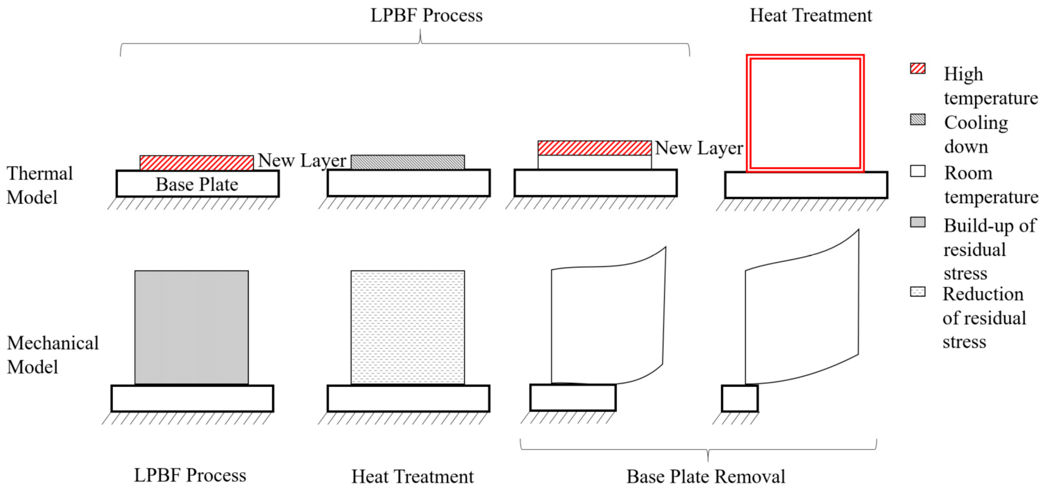
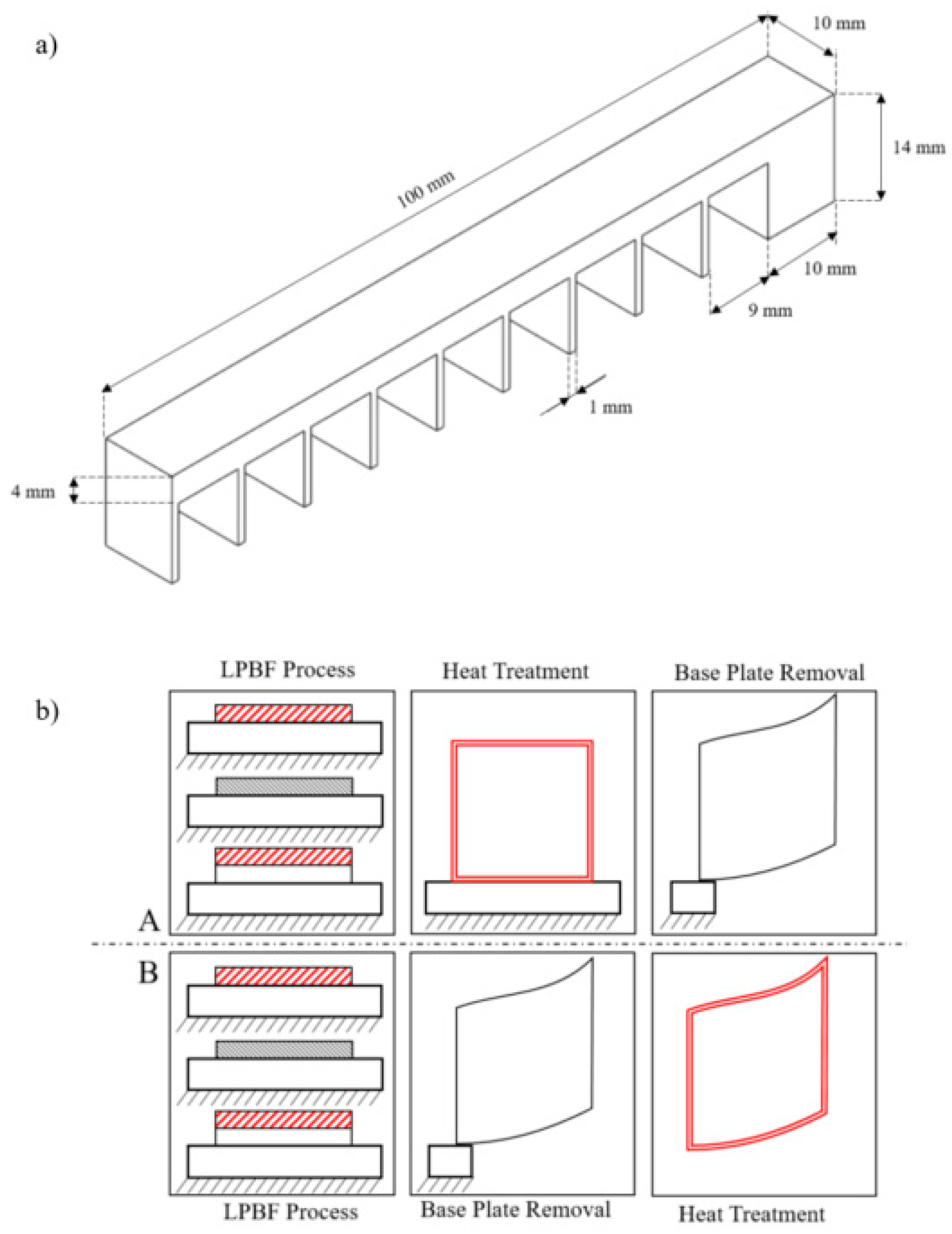
2.1. Modelling Approach

In this section, the numerical model is introduced. As mentioned in the introduction, the model in this work is a reduced fidelity model, in order to gain computational speed. The model is set up in the commercial finite element (FE) software suite ANSYS Academic Research Mechanical, release 2019 R2, using the built-in AM capabilities. The following section will go through the modelling methodology used for this module and the coupling with the subsequent heat treatment. To speed up the simulations, the elements used for this work are cubical. Features with a size smaller than the cubic element size cannot be simulated, but part-scale deformations can be simulated with relatively high resolution.

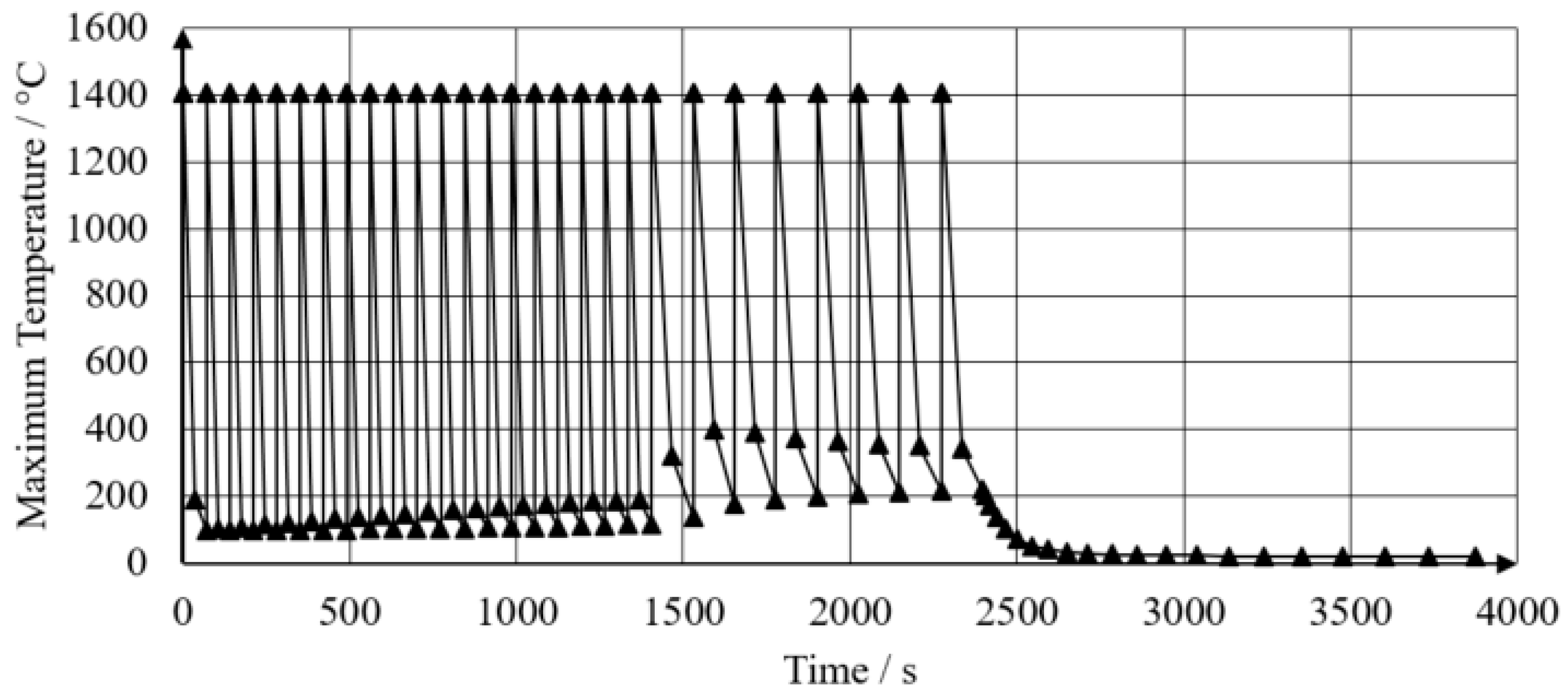
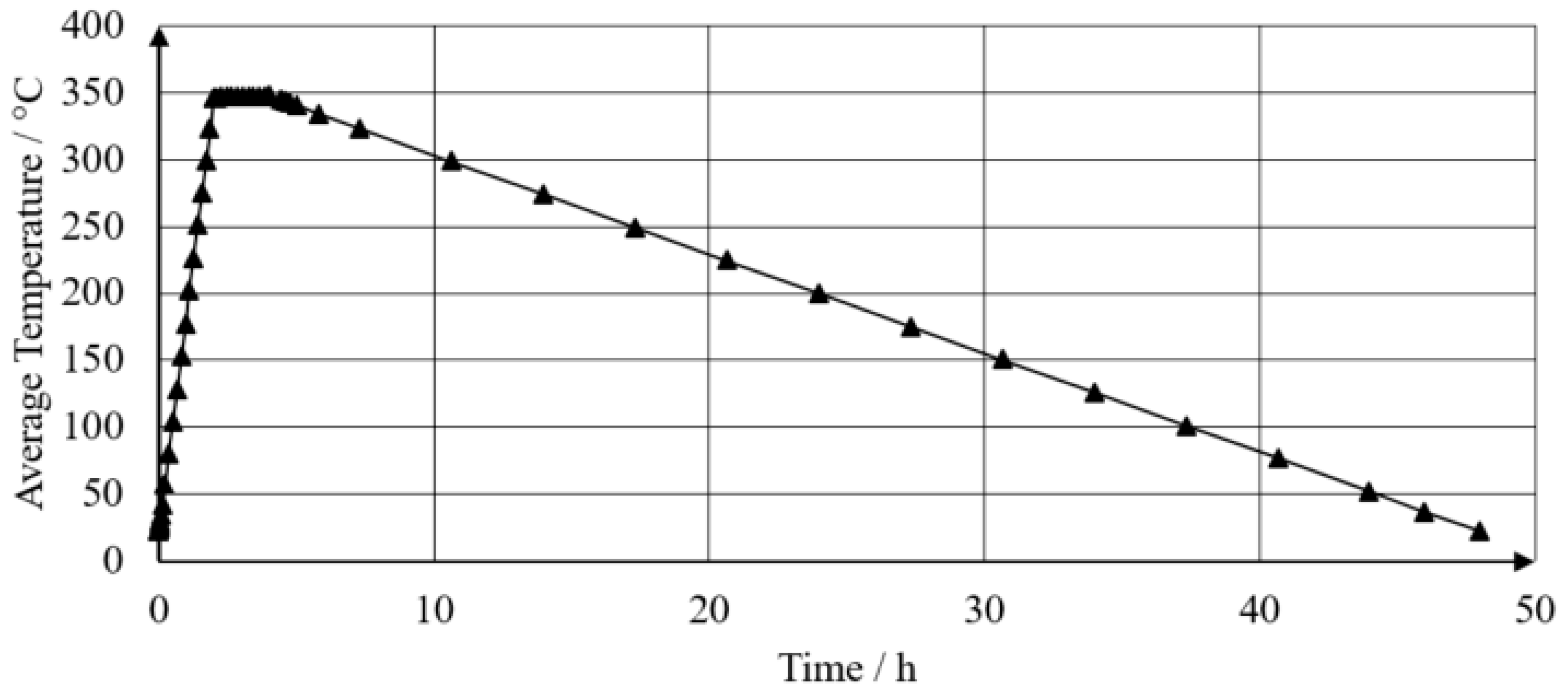
2.1.1. Thermal Model

As per usual, the basis of the thermal model used in this work is the transient heat conduction equation:

$$\begin{array}{c}\rho C_p\frac{\partial T}{\partial t}=\frac{\partial }{\partial x}\left(k\frac{\partial T}{\partial x}\right)+\frac{\partial }{\partial y}\left(k\frac{\partial T}{\partial y}\right)+\frac{\partial }{\partial z}\left(k\frac{\partial T}{\partial z}\right)\end{array}$$

(1)

where $\rho$ is the density of the material, $C_p$ the specific heat capacity and $k$ the thermal conductivity. $\rho ,C_p$and $k$are all temperature dependent.

In the model used to represent the LPBF process, the temperature is applied to the simulated part by introducing a layer of elements at an elevated temperature. Each layer of elements represents a number of real layers. This element layer is, by default, deposited at the melting temperature of the material under investigation. When cooling down, the heat from this layer is partially dissipated through the gaseous atmosphere and powder surrounding the part, and partially through underlying, earlier deposited layers, heating them up in the process. Out of these possible mechanisms, most heat will be conducted through the already completed sections of the part, since the solid material conducts more heat than the surrounding powder [18,43]. To reduce the need for simulating the powder surrounding the part, this mechanism is ignored in the presented simulations. The assumption underlying the deposition of the molten layers is that each material point in one of these new elements will have reached the melting temperature during the real process as well. This assumption will be investigated in this study.

After the LPBF process is completed, the part is allowed to cool down to room temperature, via the fixed temperature boundary conditions at the surfaces exposed to the furnace, i.e., the surfaces of the part, and the top of the base plate, on which the part is constructed.

In this work, two essential post processes are included in the process chain simulation: the cutting process and a possible stress relief heat treatment at 350 °C. The cutting process involves element death of the base plate and will be further discussed in the section on the mechanical model. In the heat treatment, the part is heated up to the heat treatment temperature in two hours, after which it is kept at this temperature for another two hours. Afterwards, the part is cooled down slowly, to ensure homogeneous cooling and no local stress build-up, which could result in new thermal stresses.

The temperature cycle is applied to the part via a fixed temperature boundary condition to the external faces of the part. This temperature profile is presented in the result section.

2.1.2. Mechanical Model

The mechanical model solves the generalised Hooke’s law in Equation (3), together with the static equilibrium in Equation (2):

$$\begin{array}{c}{\sigma }_{ij,j}=0\end{array}$$

(2)

where ${\sigma }_{ij}$ is the stress, and $i$ and $j$represent the x, y and z directions.

$$\begin{array}{c}{\sigma }_{ij}=\frac{E}{1+\nu }\left[\frac{1}{2}\left({\delta }_{ik}{\delta }_{jl}+{\delta }_{il}{\delta }_{jk}\right)+\frac{\nu }{1-2\nu }{\delta }_{ij}{\delta }_{kl}\right]{ϵ}_{kl}^{el}\end{array}$$

(3)

in which $E$represents the elasticity modulus, $\nu$the Poisson modulus, ${\delta }_{ij}$the Kronecker delta and ${ϵ}_{kl}^{el}$ the elastic strain component. Both Equation (2) and Equation (3) use the Einstein convention of summation over like indices. Besides the elastic strain, the total strain is also composed of contributions from the plastic and thermal strain:

$$\begin{array}{c}{\dot{ϵ}}_{ij}^{total}={\dot{ϵ}}_{ij}^{el}+{\dot{ϵ}}_{ij}^{pl}+{\dot{ϵ}}_{ij}^{th}\end{array}$$

(4)

Equation (4) indicates that the increase in the total strain is obtained by summation of the increments of all other strain components. The plastic strain increment follows a bilinear isotropic hardening law, using the standard J2 flow theory:

$$\begin{array}{c}{\dot{ϵ}}_{ij}^{pl}=\frac{9}{4{\sigma }_e^2}\left[\frac{E-E_t}{E{E}_t}\right]\dot{\sigma }{s}_{ij}{s}_{kl}\end{array}$$

(5)

The plastic strain increment is responsible for the permanent deformation during the LPBF process. The coupling to the temperature calculation is accomplished via the thermal strain, denoted ${ϵ}_{ij}^{th}$ in Equation (4):

$$\begin{array}{c}{\dot{ϵ}}_{ij}^{th}=\alpha {\delta }_{ij}\dot{\mathrm{T}}\end{array}$$

(6)

where $\alpha$ is the isotropic coefficient of thermal expansion, ${\delta }_{ij}$is once again the Kronecker delta, while $\dot{\mathrm{T}}$ is the temperature increment.

During the LPBF process and the stress relief heat treatment, Equation (2) to (6) are solved using the temperature obtained from the thermal calculation as an input for Equation (6) and to calculate all temperature dependent parameters. During the heat treatment simulation, stress relaxation at a temperature above 300 °C is enabled.

The final simulated post-process is the removal from the base plate. For this, the elements in the base plate are killed in an order, representative of the direction in which the band saw cuts the connection between the base plate and the desired part. In order to make sure the computational speed is retained, the elements of the base plate are killed in relatively large bunches, of 10 mm each. During the deletion of each of the regions of the base plate, the stresses are relieved until static equilibrium is reached. A schematic of the entire simulation is shown in Figure 1.

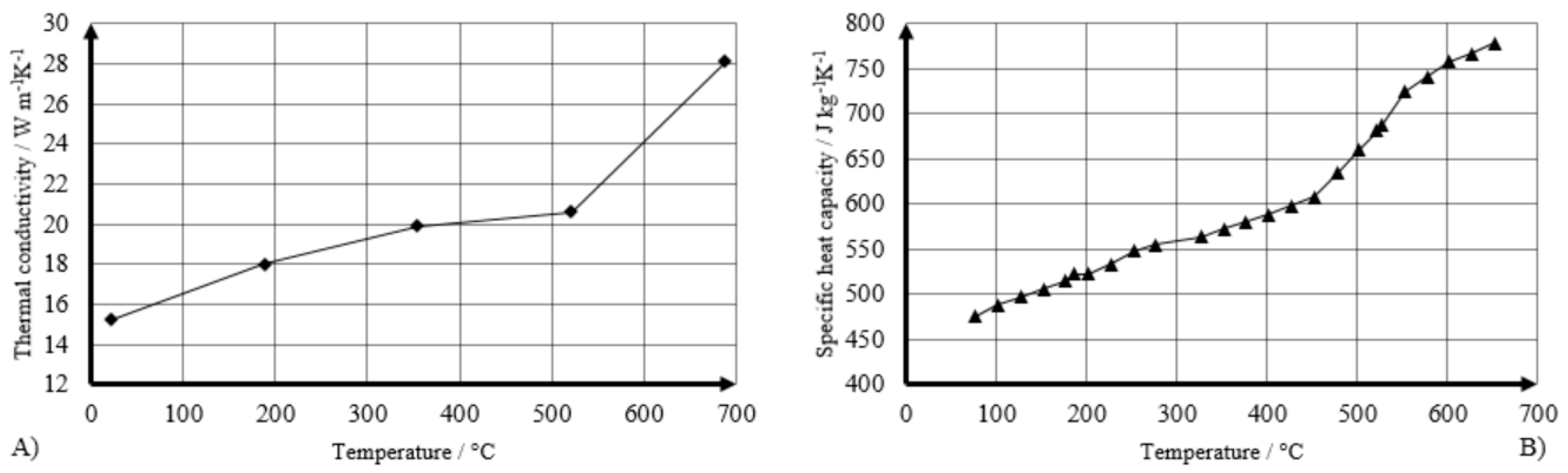
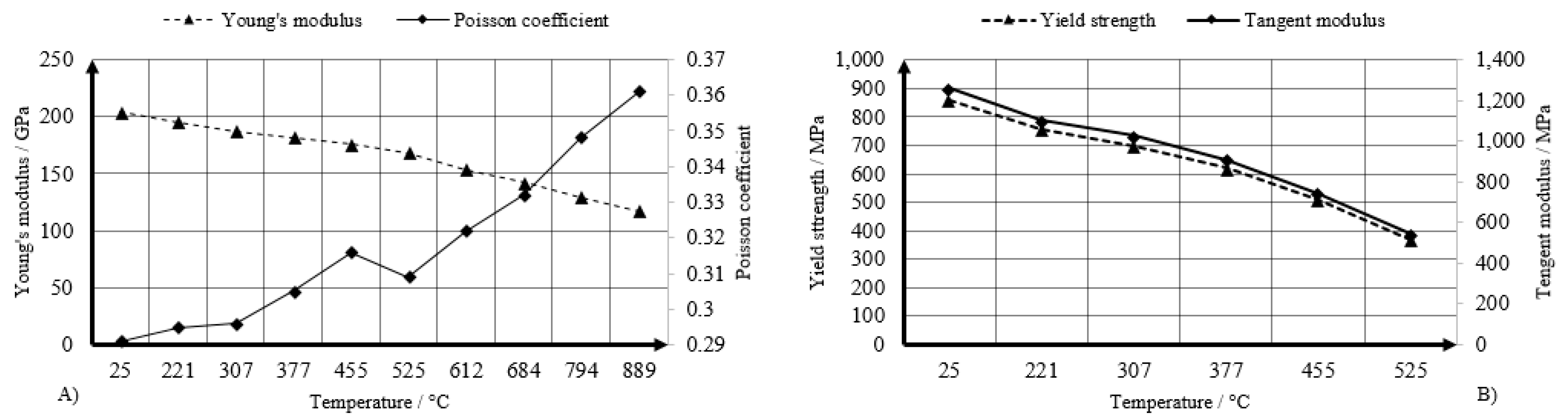
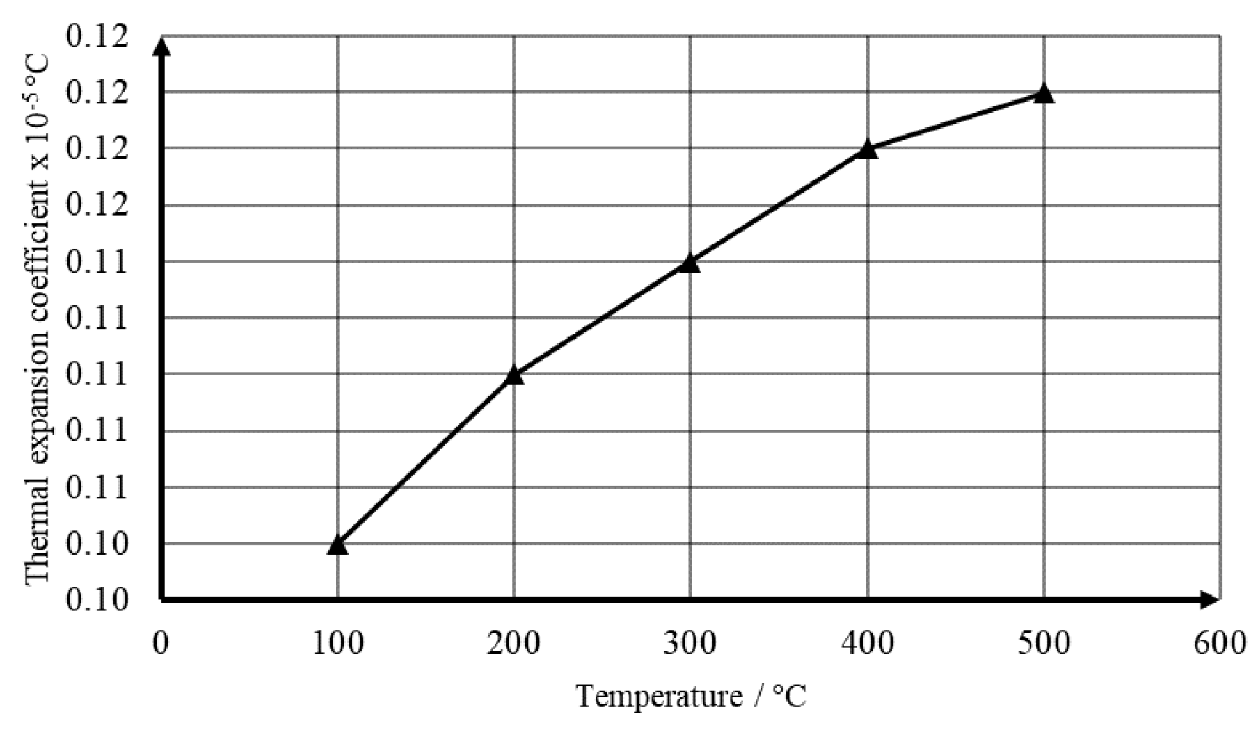
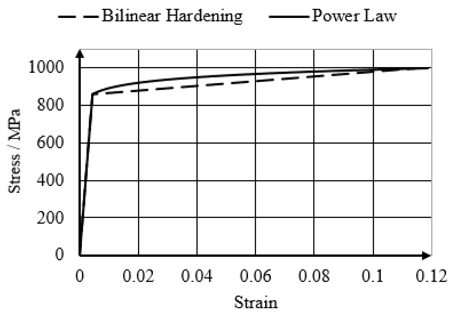
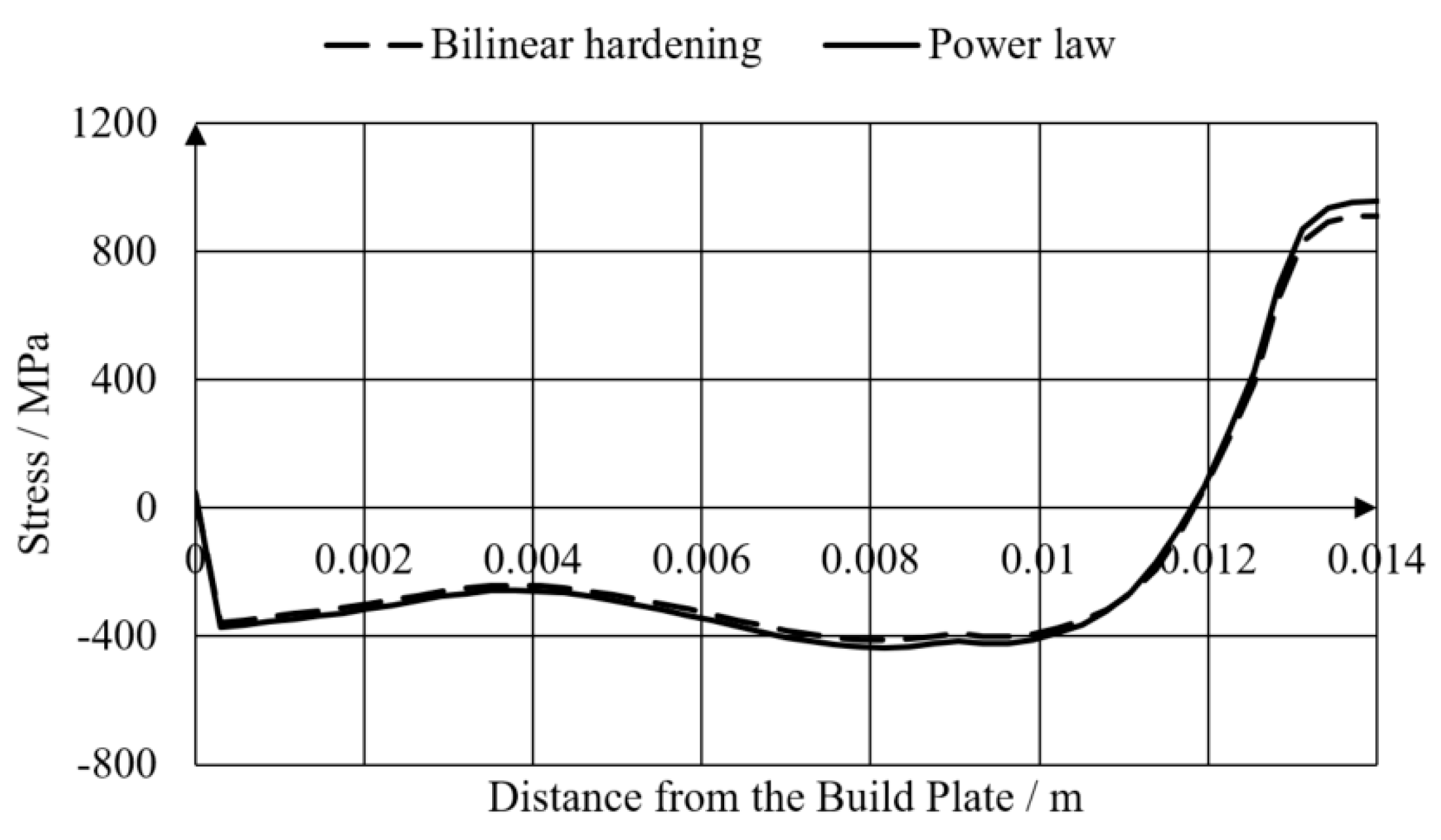
2.2. Material Properties

The material used for this study is 17-4PH stainless steel. This material has a high hardness after aging [44] and can be additively manufactured [12,45]. The parameters used in Equation (1), (3), (5), and (6) are all temperature dependent, which is of major importance for accurately predicting the stresses during LPBF due to the rapidly changing temperature during the process.

The values for the thermal conductivity and specific heat capacity are given in Figure 2A,B. The density is independent of temperature at 7790 kg m³. The parameters for the mechanical model are presented as functions of temperature in Figure 3A,B.

The value of the thermal expansion coefficient is given in Figure 4.

3. Results and Discussion

3.1. Overview of the Simulations

The current study aims to evaluate the presented model in terms of heat treatment temperature and dwell time. Four sets of simulations were performed to investigate the following: mesh convergence, dwell time, temperature and an energy correction approach for the LPBF process. To simplify the discussion on the different simulations, these are numbered according to

Table 1. Overview of all the simulations performed for this study. Note that study 1 is the simulation benchmark.

Number	Parameters				Intentions
	Time	Peak Temperature	Deposition Temperature	Element Size
1	7200 s	350 °C	1405 °C	5.00 × 10−3 m	Simulation benchmark
2	7200 s	350 °C	1405 °C	6.00 × 10−4 m	Investigation of mesh convergence
3	7200 s	350 °C	1405 °C	7.50 × 10−4 m
4	7200 s	350 °C	1405 °C	8.00 × 10−4 m
5	7200 s	350 °C	1405 °C	1.00 × 10−3 m
6	3600 s	350 °C	1405 °C	5.00 × 10−4 m	Investigation of effect of dwell time during heat treatment
7	10800 s	350 °C	1405 °C	5.00 × 10−4 m
8	7200 s	400 °C	1405 °C	5.00 × 10−4 m	Investigation of effect of heat treatment temperature
9	7200 s	300 °C	1405 °C	5.00 × 10−4 m
10	7200 s	280°C	1405 °C	5.00 × 10−4 m
11	7200 s	350 °C	3000 °C	5.00 × 10−4 m	Energy correction approach

, with associated values for the parameters. Table 1 also shows the intention of each of the simulations performed.

3.2. Benchmark Case: Simulation 1

Simulation 1 is treated as the benchmark case in this study. The part under consideration is a cantilever beam, since the expected deformation is almost exclusively in a single plane. The plane in question is the x-z plane, where the x-direction is longitudinal, and the z-direction is perpendicular to the build plate. This allows direct comparison between the obtained results. The cantilever used in this work is shown in Figure 5a. The part presented in Figure 5a cannot be easily produced in the shown orientation. It would require support underneath the large overhangs, which have a length of 9 mm. However, for the sake of these simulations, which are mostly concerned with the deformation of the cantilever beam itself, the manufacturability of the simulated geometry was not taken into account. Moreover, an easily identifiable stress field, as present in a cantilever beam was prioritised. In addition, the FE model, as presented in the preceding section, does not include effects such as dross formation or sagging. These can be identified when performing high-fidelity simulations with the associated high computational cost.

On each simulated build plate, two different process sequences are simulated. Sequence A is the theoretically preferred sequence, where the part is heat treated to relief the residual stresses and subsequently cut from the base plate. In sequence B, the order of these post-processes is reversed, although this will result in an increase of the deflection of the cantilever tip. Moreover, cutting from the cantilever from the base plate will release the residual stresses, allowing the part to deform freely. If the stresses have been reduced during stress relaxation, this will imply a reduction in the cantilever tip deflection. However, sequence B is often preferred in industry, since after heat treatment of parts in 17-4 PH stainless steel, the hardness of the part increases, to a degree where it becomes impractical to cut the part from the base plate using a mechanical machining device (such as a band saw). Both of these sequences are schematically described in Figure 5b.

Other techniques, such as electrical discharge machining (EDM) [47], will affect the stress field in a different way. EDM is an electrochemical process that can locally heat up the part and consequently locally affect the residual stresses, similar to the heat treatment itself. However, this work focusses on the aforementioned mechanical machining.

The temperature simulation during the LPBF process is summarised in Figure 6. It shows the maximum temperature in the computational domain throughout the primary LPBF process. The maximum temperature reached during the process is the melting temperature of 1405 °C. This is expected, since the initial temperature in each element layer is the melting temperature, and there is no other heat source present in the simulation, which could increase the temperature. The graph in Figure 6 also shows the peaks in temperature, which are characteristic for the LPBF process. As expected, the number of peaks corresponds to the number of deposited element layers.

Figure 7 shows the average temperature during the heat treatment. The temperature follows the imposed boundary condition, but obviously lags behind the prescribed profile.

The remainder of this section will focus on the deformations and stresses in the part. Figure 8A shows the normal stresses in the longitudinal direction before the cantilever beam is cut from the base plate. The stresses in Figure 8A are shown at the surface of the part. As predicted, the stress at the top of the cantilever is in tension, while the bottom of the cantilever is subjected to compressive stress. Figure 8B shows the same longitudinal stresses in the centre of the first support for the horizontal beam, demonstrating the evolution from compressive to tensile stress. This is also illustrated in the normal stress on the cross-section of the cantilever in Figure 8D. It shows that the transition from compression to stress only occurs relatively close to the top surface of the part. Comparing the stress in Figure 8A to the one obtained by Li et al. [5] shows a similar profile of the stress field. When looking at the left-most support, the stress is highest on the top and the bottom, while dipping in between the two maxima. However, the precise value of the stress does differ; the simulations in this work predict a maximum stress, which is about three times larger: 1026 MPa compared to 330 MPa. This is most likely due to the different choice in material: Li et al. use an aluminium-silicon alloy, with a different thermal expansion coefficient, Young’s modulus and yield strength. Similar stress profiles are shown in the works by Hodge et al. [48], Mercelis and Kruth [49], Ghosh et al. [50] or experimentally by Ganeriwala et al. [51]. However, the work by Yakout et al. [24] indicates that this approach to model the LPBF process will result in an overprediction of the residual stress, both in the longitudinal and transversal directions. Additionally, the stresses in both beams before the post-processing are identical (illustrated in Figure 8C), allowing an easy evaluation of the effect of the change of the post-processing sequence.

Finally, the deformation and stresses in the part after its release from the build plate are discussed. Comparing the stress before and after the part is heat treated but still attached to the build plate reveals that the maximal stress in the cantilever beam did not decrease significantly. This is illustrated in the next paragraph. When the part is first heat treated and cut afterwards in sequence A, the tip of the cantilever is displaced in the z-direction by 9.4 mm. The difference between the displacement observed in the cantilever which is treated according to sequence A and the cantilever which is subjected to the reverse sequence, B, is 19.3 mm. Both cantilevers are shown side by side in Figure 9, showing the clear difference in displacement. This benchmark simulation took 52 min and 13 s to complete on eight cores of an Intel Xeon W-2195 processor.

The origin of the difference of displacement must lie in the stress relaxation, which occurs during the stress relief heat treatment. The cantilever subjected to sequence B is free to move, and as a result, it will bend upwards under the influence of the residual stresses after the LPBF process. After the stress relaxation, the stresses in both cantilevers are an order of magnitude lower than after the primary process. However, when cooling slowly, new stresses build up. In the case of sequence A, the part is still attached to the base plate, and therefore, the stress profile is similar to the original one, but the absolute value is reduced. The part subjected to sequence B is free to deform, since it is already cut from the build plate. However, due to its curvature, it will deform non-homogeneously, leading to a new build-up of stresses. When undergoing the stress relief heat treatment, these new stresses are also reduced in magnitude, meaning that the cantilever will not bend back into its original deformed shape, since the stresses required to make this happen are no longer present. This leads to an increase in the deformation when comparing both cantilevers. The final profile of the longitudinal normal stress for both cantilevers after the post-processing is shown on the deformed geometry in Figure 10. This profile clearly illustrates the release of stress that occurs during the base-plate removal process. Comparing the stress profile in Figure 8C and Figure 10 illustrates this reduction in the stress field.

These results can be compared with experimental works in which the residual stresses are measured in the part. Mugwagwa et al. [52] investigated the surface residual stresses in a cuboid fabricated in Maraging steel 300, a tool steel similar to 17-4PH stainless steel. For most scanning speeds they find stresses which are larger than the ones reported in this work, namely around 300 MPa. Similarly, Massoomi et al. [53] measured the residual stress throughout a beam attached to the build plate and found a variation from tensile at the top of the beam to compressive near the bottom. This is in agreement with the results presented in Figure 8. However, they measured an increase of the stress at the bottom of the beam. Such behaviour can also be observed in Figure 8A at the surface of the part. The values of the stress at both surfaces are 153.3 MPa and 223.6 MPa at the top and bottom surfaces of the beam respectively. This is similar to the values displayed in Figure 10 at the top and bottom of the cantilevers. Barros et al. [54] investigated the residual stress through a part as well and found a similar profile, although the exact values differ, probably due to the use of Inconel 718.

To evaluate the effect of the choice of plasticity model, the same simulation is performed, but rather than bilinear hardening, a power-law plasticity model is used. The power law description of the stress strain curve is slightly more accurate in describing the uniaxial tensile behaviour of 17-4PH. The new model describes the total strain in the plastic region as follows:

$$\begin{array}{c}ϵ=\frac{{\sigma }_y}{E}{\left(\frac{\sigma }{{\sigma }_y}\right)}^n\end{array}$$

(7)

where ${\sigma }_y$ is the yield stress, $E$ the elasticity modulus and $n$the hardening exponent. The hardening exponent is fixed at a value of 22 [55]. The curves for the bilinear hardening and power law hardening at 200 °C are shown in Figure 11. Figure 12 shows the evolution of the longitudinal normal stress in the left support after the LPBF process. The tensile stress at the top of the cantilever is slightly higher when using the power law and is compensated by a slightly larger compressive stress in the bulk of the support as well.

Even though the power law description of the stress-strain curve corresponds more closely to a traditional curve for 17-4PH, it predicts a stress which is higher in absolute value throughout almost the entire domain. Yakout et al. [24] showed that the modelling approach used for the LPBF process tends to predict residual stresses which are higher than the ones expected from measurements. Therefore, the bilinear hardening law is maintained throughout this work, since its prediction of the residual stress is lower, and this is expected to be closer to experimentally obtained values.

3.3. Mesh Sensitivity Analysis: Simulations 1–5

In order to assure that the solution of the simulation is not heavily dependent on the mesh, a mesh sensitivity analysis is performed. Five different element sizes are used, namely 1e-3 m, 8e-4 m, 7.5e-4 m, 6e-4 m and 5e-4 m. This last simulation is the previously discussed benchmark simulation. Yakout et al. [24] investigated the mesh independency of the primary LPBF process and showed that the method implemented in ANSYS Academic Research Mechanical, release 2019 R2, becomes independent for the smallest element size chosen. However, this work will evaluate the same for the two post-processing steps. The metric chosen to evaluate the mesh sensitivity is the stress in the left support at the top of the cantilever.

Table 2. The values of the maximal longitudinal normal stress after the entire process chain (sequence A).

Simulation Number	1	2	3	4	5
Element size (m)	5 × 10−4	6 × 10−4	7.5 × 10−4	8 × 10−4	1 × 10−3
Longitudinal normal stress (MPa)	841.6	840.5	835.1	832.8	825.7

shows the values of the aforementioned metric for all five simulations for process sequence A. It shows that the stress increases for a finer mesh, indicating that the longitudinal normal stress is overestimated at the top of the cantilever for a too coarse mesh. However, the values show a clear convergent behaviour, indication that a finer mesh results in a mesh-independent solution. In this work, to ensure that the simulations remain computationally inexpensive, the mesh size of the part is kept at 5e-4 m, which is the finest mesh used for the presented simulations.

3.4. Effect of the Duration of the Heat Treatment: Simulations 6 and 7

The following simulations attempt to evaluate the capability of the model to capture the effect of two key parameters for heat treatment of the additively manufactured part: the duration of the stress relief heat treatment and the temperature of the heat treatment. First, the duration is investigated.

In simulation 6, the dwell time of the heat treatment is reduced to one hour, while simulation 7 uses a 3-h holding time. These two simulations are compared to the original stress relief heat treatment, which has a two-hour holding time.

The short heat treatment has identical deflections and stresses compared to the benchmark, for both process sequences. This shows that the majority of the stress relaxation takes place in a span of one hour. The model predicts that a heat treatment of one hour is sufficient to relax all the stresses in the part.

For both the beam subjected to sequence A and sequence B, the deflection of the tip of the beam for simulation 7 is larger than the same deflection for simulation 3. Focussing on sequence A, the change in the deflection is found to be less than ten percent, and the change in the stress is similarly low. To find the reason for this difference, the stress at the centre of the top surface of the cantilever is plotted in Figure 13 for both simulations 1 and 7. It is clear from this plot that the stresses are reduced during the high-temperature part of the stress relaxation. On the other hand, the stress is restored upon cooling back down to room temperature, although they are more homogeneous, which can be seen by comparing Figure 11 with Figure 8A. The small difference in the deformation results from the small change in stress, which results from the reduction that follows the stress relaxation. The results also indicate that the stress relaxation is calculated from the beginning of the heat treatment and instantly applied.

3.5. Effect of the Heat Treatment Temperature: Simulations 8, 9 and 10

The second parameter, which is important during heat treatment, is the chosen temperature. The aim from a practical point of view is to reduce the temperature. Choosing a lower temperature means that less energy is required to heat up the part and the furnace to the desired temperature, and less time is necessary to cool it down, while still retaining the same low cooling rate when cooling down, resulting in similarly homogeneous stresses. In this study, three additional temperatures are chosen for stress relaxation. To probe the model and evaluate its capability with respect to the temperature, one heat treatment is simulated at 400 °C and one at the lowest possible temperature above the relaxation temperature, which is 300 °C. Finally, a heat treatment below the relaxation temperature is simulated at 280 °C.

The results from these three simulations are collected in

Table 3. Data from simulations 8, 9 and 10.

		Simulation 8			Simulation 9			Simulation 10
Temperature		400 °C			300 °C			280 °C
	Sequence A		Sequence B	Sequence A		Sequence B	Sequence A		Sequence B
Displacement in z (m)	0.0102		0.0363	0.0102		0.0364	0.0102		0.0103
End stress (Pa)	1.00 × 109		1.28 × 109	1.39 × 109		1.28 × 109	1.00 × 109		1.10 × 109

, using the following metrics: the displacement of the tip of the cantilever and the maximum normal stress in the longitudinal direction at the end of the entire process chain, for both sequence A and B. First, focussing on simulations 8 and 9 shows that both of these stress relaxation treatments lead to similar displacements of the free end of the cantilever. Performing stress relaxation at a lower temperature does lead to a slight increase in the normal stress, most particularly in sequence A. The increase in the stress indicates that heating to any temperature above the stress relaxation temperature will lead to a similar degree of geometrical accuracy. However, looking at simulation 10 reveals what happens when the stress relief heat treatment does not exceed the stress relaxation temperature. In simulation 10, both cantilevers bend upwards with the same amount. Contrary to all previous cases, the order of the post-process does not affect the final geometry. This also provides insight into the reason why sequence B is inferior for the geometrical precision for a horizontal cantilever beam. Due to the increase in temperature during a stress relief heat treatment, if the part is removed from the base plate before it is heat treated, the bending of the beam will increase. During the heat treatment, the bottom of the beam will expand more than the top since it is longer due to the released residual stresses (and the associated bending). This will lead to a gradient in stress from the bottom of the part towards the top: the bottom is compressed, which changes to tension while moving to the top of the cantilever. If the stress were not relaxed during the heat treatment, this stress would disappear when cooling back down to room temperature, and the beam will bend back to its original shape, illustrated by the small difference in z-displacement between sequence A and sequence B in simulation 10. However, when stress relaxation does occur, these compressive and tensile stresses disappear. When cooling down to room temperature, new stresses build up, which prevent the part from returning to its original shape, leading to a permanent increase in the deflection of the cantilever beam tip.

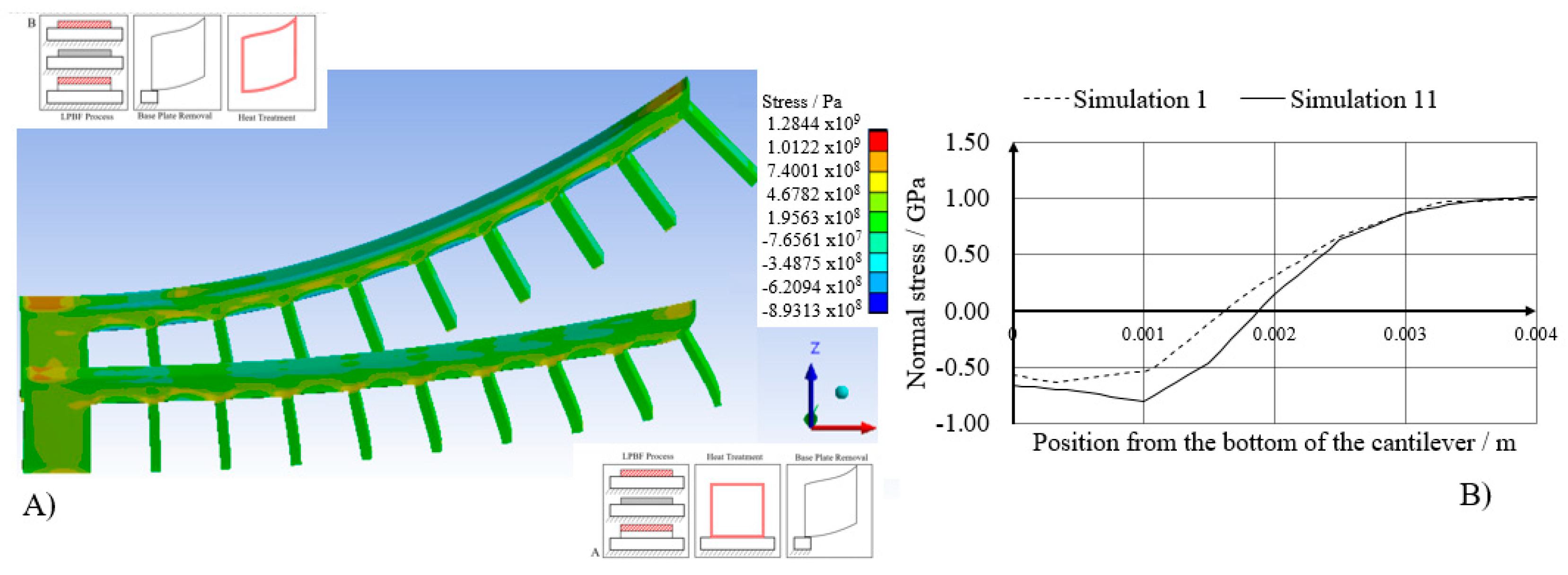
3.6. Correcting the Energy Input of the Primary Process: Simulation 11

In the original implementation of the LPBF process, every layer of elements is deposited at the melting temperature of the metal, which for 17-4PH stainless steel is 1405 °C. The energy associated with elevating a layer of elements from room temperature to the melting temperature can be calculated as follows:

$$\begin{array}{c}{E}_{simul}=\rho V\underset{T_{room}}{\overset{T_m}{{\displaystyle \int }}}{C}_{p}dT\end{array}$$

(8)

where $V$ is the volume of the part, and $T_{room}$ and $T_m$are the room and the melting temperature respectively. For a 1e-3 m³ cube, this energy equates to 6375 kJ. On the other hand, it is possible to calculate the total transferred energy for the actual LPBF process. The total energy is equal to

$$\begin{array}{c}{E}_{real}=\frac{\alpha P}{v}\frac{V}{h\delta }\end{array}$$

(9)

In this equation, $\alpha$is the absorptivity of the powder, $P$the laser power, $v$the velocity of the laser, $V$the volume of the part, $h$the hatch spacing and $\delta$the thickness of a deposited layer. For the earlier cube, this results in an energy of 1.6e4 kJ. This is considerably higher than the energy from the simulation. This can be corrected by equating Equation (7) to Equation (8) and adding a correction term:

$$\begin{array}{c}{E}_{real}=E_{simul}+\rho C_p^{m}V\mathsf{\Delta }T\end{array}$$

(10)

where the term accounts for the overheating of each element layer, in which $C_p^m$ is the heat capacity at the melting temperature. This overheating is therefore equal to

$$\begin{array}{c}\mathsf{\Delta }T=\frac{\alpha P}{\rho vh\delta C_p^m}-\frac{1}{C_p^m}\underset{T_{room}}{\overset{T_m}{{\displaystyle \int }}}{C}_{p}dT\end{array}$$

(11)

which is incidentally independent of the volume of the cube. The value of this overheating term is 1595 °C. Therefore, the temperature in each deposited layer is set to 3000 °C. To ensure no stresses build up in the part while it is still molten, the stress-free temperature is set to the melting temperature of the part, i.e., 1405 °C.

The results of the entire simulation when using this correction term are shown in Figure 14A. When comparing the stresses displayed in this figure with the ones from the earlier simulation, shown in Figure 8A, the stress and displacement are comparable, which reinforces the effectiveness of the stress relaxation temperature as a measure to increase reproducibility for the geometrical precision of a part. Figure 14B shows the normal stress along the cantilever for simulation 1 and 11. The stress is plotted from the bottom of the cantilever to the top. This shows that, even though the behaviour of the stress profiles are similar for both, and the compressive stress at the bottom is similar, the tensile stress at the top of the cantilever with corrected energy input is about two percent higher.

The results from simulation 11 are mostly relevant for modelling the LPBF process itself. For high-fidelity simulations, the energy input ought to be corrected. However, since the simulations presented in this work are reduced fidelity simulations, the correction does not significantly increase the predictive power of the model. Additionally, since the stress relaxation works as expected, namely removing high residual stresses, the difference between the two simulations becomes negligible, both in terms of the deformation of the part and the residual stresses after the entire process chain.

4. Conclusions

Simulation of the AM process chain has great applicability in an industrial environment, where the goal is to achieve high quality products, and for this a holistic view of the influence of each step of the chain is required. In this study, a section of the LPBF process chain is modelled and investigated. The simulations are set up in ANSYS Academic Research Mechanical, release 2019 R2, and include the primary process and two post-processes: removal of the part from the base plate and a stress relaxation heat treatment. To analyse the effect of the order of the post-processes, two sequences are proposed: sequence A, in which the part is first heat treated and subsequently removed from the base plate, and sequence B, in which the reverse order of these operations takes place. The model is also probed in terms of two parameters, namely the temperature of the heat treatment and the duration of the same. Additionally, a procedure is proposed to improve the prediction of the primary process by using a corrected deposition temperature. The temperature is calculated by matching the energy input of a molten element layer, with the energy that is absorbed by the powder during the real process. The results lead to the following conclusions.

• The model is capable of modelling the entire process in a limited amount of time and using a limited amount of computational resources. This allows a large number of simulations to be run for estimating the effect of varying certain parameters.
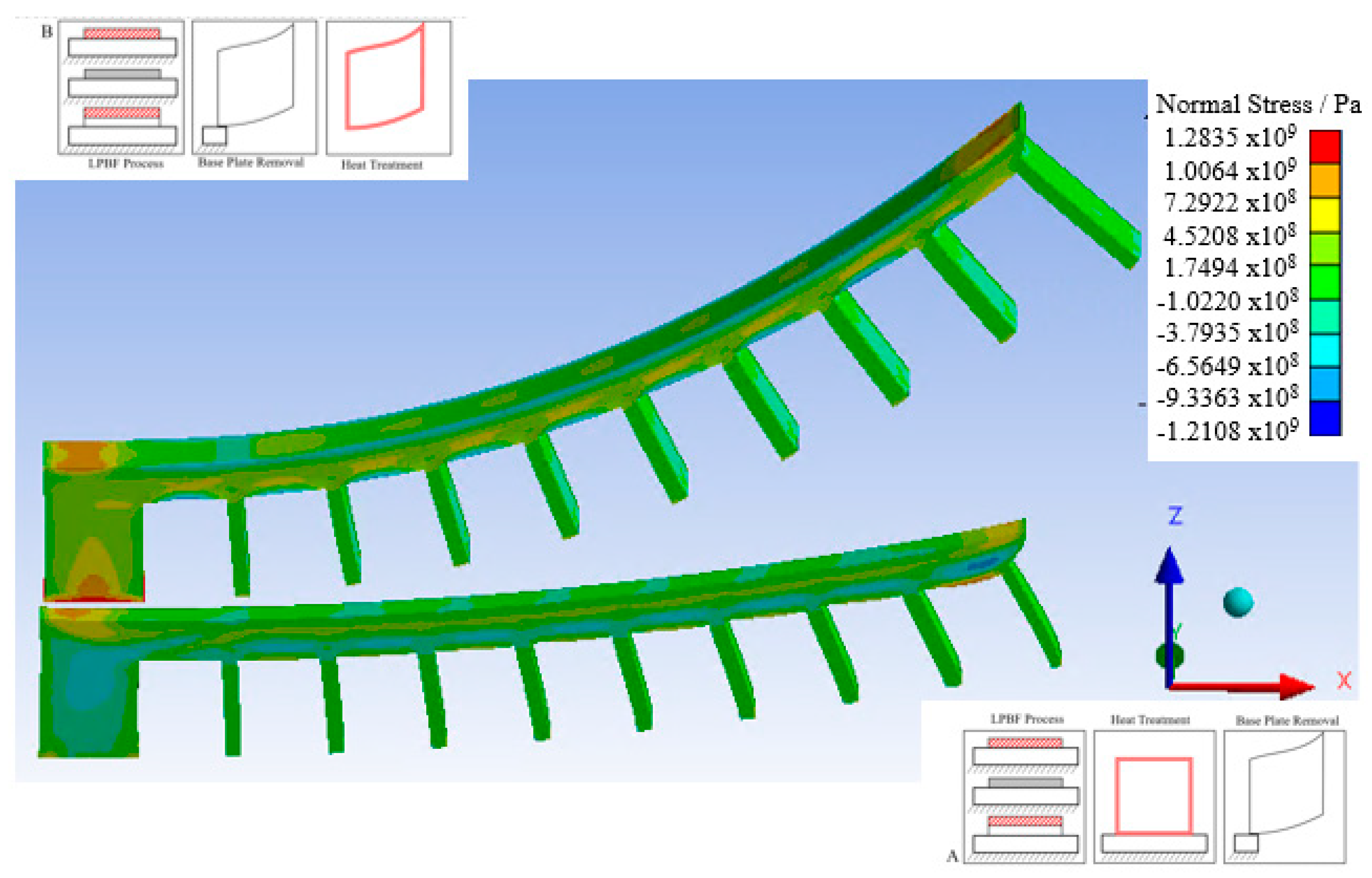
• The effect of changing the process chain sequence, from first heat treating to first removing from the base plate, leads to an increase of the deformation of the used part. This is most likely due to the stress relaxation, which causes deformation without build-up of stresses when heating up, while causing a build-up of stress and limited deformation when cooling down.
• The model also illustrates the capabilities of a generic FE solver to show the effect of the different process chain steps in the additive manufacturing process chain on the part quality.
• The model is not capable of capturing the effect of the duration of the heat treatment or the used temperature accurately due to its insensitivity to these parameters. However, when heating below the relaxation temperature a significant difference is observed in sequence B, since the stresses are no longer relaxed when heating up the beam.
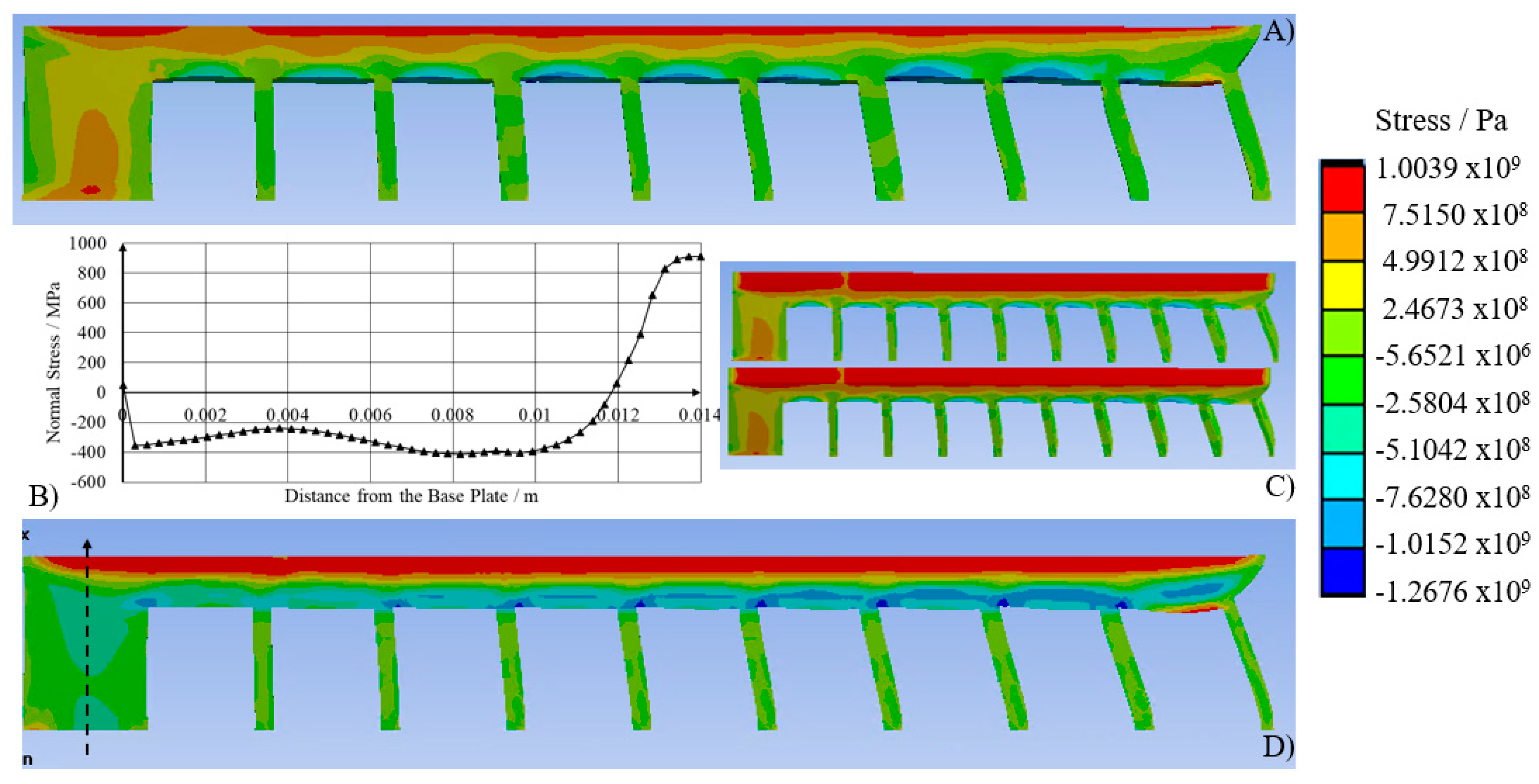
• The stress relaxation does not decrease the stresses in a cantilever beam significantly but does lead to a homogenisation of this stress.
• Correcting the energy input does lead to an improved estimate for the residual stress in the part before post-processing, but since the post-processing changes the stress, the final deflection of a cantilever beam-type part does not differ significantly.

Using a general purpose FE software package offers great flexibility in an industrial environment. This research demonstrates the capability of such software to provide reasonably reliable results, without the requirement to purchase typically expensive packages dedicated to the LPBF process. Using this FE solver also presents future opportunities to extend the simulation, covering additional post-process steps, for example milling or polishing, using only a single simulation programme [1].

References

1. Wohlers, T. Wohlers Report 2018. Tech. Rep. 2018. [Google Scholar]
2. Klocke, F.; Arntz, K.; Teli, M.; Winands, K.; Wegener, M.; Oliari, S. State-of-the-art Laser Additive Manufacturing for Hot-work Tool Steels. Procedia CIRP 2017, 63, 58–63. [Google Scholar] [CrossRef]
3. Liu, S.; Shin, Y.C. Additive manufacturing of Ti6Al4V alloy: A review. Mater. Des. 2019, 164, 107552. [Google Scholar] [CrossRef]
4. Williams, R.J.; Davies, C.M.; Hooper, P.A. A pragmatic part scale model for residual stress and distortion prediction in powder bed fusion. Addit. Manuf. 2018, 22, 416–425. [Google Scholar] [CrossRef]
5. Li, C.; Liu, J.; Fang, X.; Guo, Y. Efficient predictive model of part distortion and residual stress in selective laser melting. Addit. Manuf. 2017, 17, 157–168. [Google Scholar] [CrossRef]
6. Ahmad, B.; Van Der Veen, S.; Fitzpatrick, M.; Guo, H. Residual stress evaluation in selective-laser-melting additively manufactured titanium (Ti-6Al-4V) and inconel 718 using the contour method and numerical simulation. Addit. Manuf. 2018, 22, 571–582. [Google Scholar] [CrossRef]
7. Markl, M.; Körner, C. Multiscale Modeling of Powder Bed–Based Additive Manufacturing. Annu. Rev. Mater. Res. 2016, 46, 93–123. [Google Scholar] [CrossRef]
8. Kruth, J.; Froyen, L.; Van Vaerenbergh, J.; Mercelis, P.; Rombouts, M.; Lauwers, B. Selective laser melting of iron-based powder. J. Mater. Process. Technol. 2004, 149, 616–622. [Google Scholar] [CrossRef]
9. Ferguson, B.; Li, Z.; Freborg, A. Modeling heat treatment of steel parts. Comput. Mater. Sci. 2005, 34, 274–281. [Google Scholar] [CrossRef]
10. Dong, P.; Song, S.; Zhang, J. Analysis of residual stress relief mechanisms in post-weld heat treatment. Int. J. Press. Vessel. Pip. 2014, 122, 6–14. [Google Scholar] [CrossRef]
11. Azizi, H.; Ghiaasiaan, R.; Prager, R.; Ghoncheh, M.; Abu Samk, K.; Lausic, A.; Byleveld, W.; Phillion, A. Metallurgical and mechanical assessment of hybrid additively-manufactured maraging tool steels via selective laser melting. Addit. Manuf. 2019, 27, 389–397. [Google Scholar] [CrossRef]
12. Makoana, N.W.; Yadroitsava, I.; Moller, H.; Yadroitsev, I. Characterization of 17-4PH Single Tracks Produced at Different Parametric Conditions towards Increased Productivity of LPBF Systems—The Effect of Laser Power and Spot Size Upscaling. Metals 2018, 8, 475. [Google Scholar] [CrossRef] [Green Version]
13. Yaghi, A.; Ayvar-Soberanis, S.; Moturu, S.R.; Bilkhu, R.; Afazov, S. Design against distortion for additive manufacturing. Addit. Manuf. 2019, 27, 224–235. [Google Scholar] [CrossRef] [Green Version]
14. Antony, K.; Arivazhagan, N.; Senthilkumaran, K. Numerical and experimental investigations on laser melting of stainless steel 316L metal powders. J. Manuf. Process. 2014, 16, 345–355. [Google Scholar] [CrossRef]
15. Bayat, M.; Mohanty, S.; Hattel, J. A systematic investigation of the effects of process parameters on heat and fluid flow and metallurgical conditions during laser-based powder bed fusion of Ti6Al4V alloy. Int. J. Heat Mass Transf. 2019, 139, 213–230. [Google Scholar] [CrossRef]
16. Bayat, M.; Mohanty, S.; Hattel, J. Multiphysics modelling of lack-of-fusion voids formation and evolution in IN718 made by multi-track/multi-layer L-PBF. Int. J. Heat Mass Transf. 2019, 139, 95–114. [Google Scholar] [CrossRef]
17. Hussein, A.; Hao, L.; Yan, C.; Everson, R. Finite element simulation of the temperature and stress fields in single layers built without-support in selective laser melting. Mater. Des. 2013, 52, 638–647. [Google Scholar] [CrossRef]
18. Parry, L.; Ashcroft, I.; Wildman, R.D. Understanding the effect of laser scan strategy on residual stress in selective laser melting through thermo-mechanical simulation. Addit. Manuf. 2016, 12, 1–15. [Google Scholar] [CrossRef] [Green Version]
19. Hodge, N.E.; Ferencz, R.; Solberg, J.M. Implementation of a thermomechanical model for the simulation of selective laser melting. Comput. Mech. 2014, 54, 33–51. [Google Scholar] [CrossRef]
20. Chen, C.; Yin, J.; Zhu, H.; Xiao, Z.; Zhang, L.; Zeng, X. Effect of overlap rate and pattern on residual stress in selective laser melting. Int. J. Mach. Tools Manuf. 2019, 145, 103433. [Google Scholar] [CrossRef]
21. Denlinger, E.R. Thermomechanical Model Development and In Situ Experimental Validation of the Laser Powder-Bed Fusion Process. Thermo-Mech. Model Addit. Manuf. 2017, 16, 215–227. [Google Scholar] [CrossRef]
22. Parry, L.; Ashcroft, I.; Wildman, R.D. Geometrical effects on residual stress in selective laser melting. Addit. Manuf. 2019, 25, 166–175. [Google Scholar] [CrossRef]
23. Bayat, M.; Klingaa, C.; De Baere, D.; Mohanty, S.; Thorborg, J.; Skat Tiedje, N.; Hattel, J.H. Part-scale thermo-mechanical modellin of distortions in L-PBF-Analysis of the sequential flash heating method with experimental validation. Addit. Manuf. 2020. (Under review). [Google Scholar]
24. Yakout, M.; Elbestawi, M.; Veldhuis, S.; Nangle-Smith, S. Influence of thermal properties on residual stresses in SLM of aerospace alloys. Rapid Prototyp. J. 2020, 26, 213–222. [Google Scholar] [CrossRef]
25. Yadroitsev, I.; Gusarov, A.; Yadroitsava, I.; Smurov, I.Y. Single track formation in selective laser melting of metal powders. J. Mater. Process. Technol. 2010, 210, 1624–1631. [Google Scholar] [CrossRef]
26. Ukar, E.; Lamikiz, A.; De Lacalle, L.L.; Martinez, S.; Liebana, F.; Tabernero; Lamikiz, A.; De Lacalle, L.N.L. Thermal model with phase change for process parameter determination in laser surface processing. Phys. Procedia 2010, 5, 395–403. [Google Scholar] [CrossRef] [Green Version]
27. Montevecchi, F.; Venturini, G.; Grossi, N.; Scippa, A.; Campatelli, G. Finite Element mesh coarsening for effective distortion prediction in Wire Arc Additive Manufacturing. Addit. Manuf. 2017, 18, 145–155. [Google Scholar] [CrossRef]
28. Bayat, M.; Mohanty, S.; Hattel, J. Numerical modelling and parametric study of grain morphology and resultant mechanical properties from selective laser melting process of Ti6Al4V. In Proceedings of the 18th International Conference of the european Society for Precision Engineering and Nanotechnology (euspen 18), Venice, Italy, 4–8 June 2018. [Google Scholar]
29. Vaverka, O.; Koutny, D.; Vrana, R. Effect of heat treatment on mechanical properties and residual stresses in additively manufactured parts. In Proceedings of the 24th International Conference Engineering Mechanics 2018, Svratka, Czech Republic, 14–27 May 2018. [Google Scholar] [CrossRef] [Green Version]
30. Shiomi, M.; Osakada, K.; Nakamura, K.; Yamashita, T.; Abe, F. Residual Stress within Metallic Model Made by Selective Laser Melting Process. CIRP Ann. 2004, 53, 195–198. [Google Scholar] [CrossRef]
31. Mutua, J.; Nakata, S.; Onda, T.; Chen, Z.-C. Optimization of selective laser melting parameters and influence of post heat treatment on microstructure and mechanical properties of maraging steel. Mater. Des. 2018, 139, 486–497. [Google Scholar] [CrossRef]
32. Rohde, J.; Jeppsson, A. Literature review of heat treatment simulations with respect to phase transformation, residual stresses and distortion. Scand. J. Met. 2000, 29, 47–62. [Google Scholar] [CrossRef]
33. Su, B.; Ma, Q.; Han, Z. Modeling of Austenite Decomposition during Continuous Cooling Process in Heat Treatment of Hypoeutectoid Steel with Cellular Automaton Method. Steel Res. Int. 2017, 88, 1600490. [Google Scholar] [CrossRef]
34. Yan, G.; Crivoi, A.; Sun, Y.; Maharjan, N.; Song, X.; Li, F.; Tan, M.J. An Arrhenius equation-based model to predict the residual stress relief of post weld heat treatment of Ti-6Al-4V plate. J. Manuf. Process. 2018, 32, 763–772. [Google Scholar] [CrossRef]
35. Alberg, H.; Berglund, D. Comparison of plastic, viscoplastic, and creep models when modelling welding and stress relief heat treatment. Comput. Methods Appl. Mech. Eng. 2003, 192, 5189–5208. [Google Scholar] [CrossRef]
36. De Baere, D.; Bayat, M.; Mohanty, S.; Hattel, J. Thermo-fluid-metallurgical modelling of the selective laser melting process chain. Procedia CIRP 2018, 74, 87–91. [Google Scholar] [CrossRef]
37. Denlinger, E.R.; Michaleris, P. (Pan) Effect of stress relaxation on distortion in additive manufacturing process modeling. Addit. Manuf. 2016, 12, 51–59. [Google Scholar] [CrossRef] [Green Version]
38. Tan, P.; Shen, F.; Li, B.; Zhou, K. A thermo-metallurgical-mechanical model for selective laser melting of Ti6Al4V. Mater. Des. 2019, 168, 107642. [Google Scholar] [CrossRef]
39. Zanger, F.; Boev, N.; Schulze, V. Novel Approach for 3D Simulation of a Cutting Process with Adaptive Remeshing Technique. Procedia CIRP 2015, 31, 88–93. [Google Scholar] [CrossRef] [Green Version]
40. Afazov, S. Modelling and simulation of manufacturing process chains. CIRP J. Manuf. Sci. Technol. 2013, 6, 70–77. [Google Scholar] [CrossRef]
41. Zaeh, M.F.; Tekkaya, A.E.; Biermann, D.; Zabel, A.; Langhorst, M.; Schober, A.; Kloppenborg, T.; Steiner, M.; Ungemach, E. Integrated simulation of the process chain composite extrusion–milling–welding for lightweight frame structures. Prod. Eng. 2009, 3, 441–451. [Google Scholar] [CrossRef]
42. Gallego, A.C.; Ramos, L.M.M.; Aguirrebeitia, J.; De Lacalle, L.N.L.; De Lacalle, L.L. A Methodology to Evaluate the Reliability Impact of the Replacement of Welded Components by Additive Manufacturing Spare Parts. Metals 2019, 9, 932. [Google Scholar] [CrossRef] [Green Version]
43. Gusarov, A.; Smurov, I.Y. Modeling the interaction of laser radiation with powder bed at selective laser melting. Phys. Procedia 2010, 5, 381–394. [Google Scholar] [CrossRef] [Green Version]
44. Hsiao, C.; Chiou, C.; Yang, J.-R. Aging reactions in a 17-4 PH stainless steel. Mater. Chem. Phys. 2002, 74, 134–142. [Google Scholar] [CrossRef]
45. Hu, Z.; Zhu, H.; Zhang, H.; Zeng, X. Experimental investigation on selective laser melting of 17-4PH stainless steel. Opt. Laser Technol. 2017, 87, 17–25. [Google Scholar] [CrossRef]
46. Ansys Workbench Release 2019 R2. Available online: https://www.ansys.com/ (accessed on 5 May 2019).
47. Sames, W.; List, F.A.; Pannala, S.; Dehoff, R.R.; Babu, S.S. The metallurgy and processing science of metal additive manufacturing. Int. Mater. Rev. 2016, 61, 315–360. [Google Scholar] [CrossRef]
48. Hodge, N.E.; Ferencz, R.; Vignes, R. Experimental comparison of residual stresses for a thermomechanical model for the simulation of selective laser melting. Addit. Manuf. 2016, 12, 159–168. [Google Scholar] [CrossRef]
49. Mercelis, P.; Kruth, J. Residual stresses in selective laser sintering and selective laser melting. Rapid Prototyp. J. 2006, 12, 254–265. [Google Scholar] [CrossRef]
50. Ghosh, S.; McReynolds, K.; E Guyer, J.; Banerjee, D.K. Simulation of temperature, stress and microstructure fields during laser deposition of Ti–6Al–4V. Model. Simul. Mater. Sci. Eng. 2018, 26, 075005. [Google Scholar] [CrossRef] [Green Version]
51. Ganeriwala, R.; Strantza, M.; King, W.; Clausen, B.; Phan, T.; Levine, L.; Brown, D.; Hodge, N. Evaluation of a thermomechanical model for prediction of residual stress during laser powder bed fusion of Ti-6Al-4V. Addit. Manuf. 2019, 27, 489–502. [Google Scholar] [CrossRef]
52. Mugwagwa, L.; Yadroitsev, I.; Matope, S. Effect of Process Parameters on Residual Stresses, Distortions, and Porosity in Selective Laser Melting of Maraging Steel 300. Metals 2019, 9, 1042. [Google Scholar] [CrossRef] [Green Version]
53. Masoomi, M.; Shamsaei, N.; Winholtz, R.A.; Milner, J.L.; Gnäupel-Herold, T.; Elwany, A.; Mahmoudi, M.; Thompson, S.M. Residual stress measurements via neutron diffraction of additive manufactured stainless steel 17-4 PH. Data Brief 2017, 13, 408–414. [Google Scholar] [CrossRef]
54. Barros, R.; Silva, F.J.G.; Gouveia, R.; Saboori, A.; Marchese, G.; Biamino, S.; Salmi, A.; Atzeni, E. Laser Powder Bed Fusion of Inconel 718: Residual Stress Analysis Before and After Heat Treatment. Metals 2019, 9, 1290. [Google Scholar] [CrossRef] [Green Version]
55. ASM International. Atlas of Stress-Strain Curves, 2nd ed.; ASM International: Russel Township, ON, Canada, 2002. [Google Scholar]
Figure 1. Schematic of the process chain model including the laser-based powder bed fusion (LPBF) process, stress relief heat treatment and removal of the base plate. Both the thermal and mechanical part of the model are depicted.
Applsci 10 03414 g001
Figure 2. Parameters for the thermal part of the finite element (FE) model; (A) thermal conductivity as function of temperature; (B) specific heat capacity. Data from [46].
Applsci 10 03414 g002
Figure 3. Parameters for the mechanical part of the FE model; (A) Young’s modulus and Poisson coefficient of 17-4 precipitation hardening (PH) stainless steel; (B) yield strength and tangent modulus as function of temperature for the bilinear hardening law used. Data from [46].
Applsci 10 03414 g003
Figure 4. Thermal expansion coefficient as functions of temperature. Data from [46].
Applsci 10 03414 g004
Figure 5. Part geometry and process sequence; (a) the cantilever part that is used throughout this study; (b) the two different process sequences analysed in this work. In sequence A (top), the heat treatment immediately follows the primary LPBF process, before the part is removed from the base plate. Sequence B (bottom) reverses the order of the heat treatment and removal from the base plate. In the simulation, the beam simulated according to sequence A is in front, while the cantilever following sequence B is in the back.
Applsci 10 03414 g005
Figure 6. The maximum temperature in the computational domain during the primary LPBF process.
Applsci 10 03414 g006
Figure 7. Average temperature in the computational domain during the stress relief heat treatment.
Applsci 10 03414 g007
Figure 8. Stress in the cantilever after the primary LPBF process; (A) the normal stress in the x-direction (longitudinal) at the surface of the part; (B) the stresses on the left-most support of the cantilever, indicated in Figure 8D; (C) the same normal stress in longitudinal direction. The stress field is identical; (D) the same stress component as Figure 8A, but on the central cross-section of the part.
Applsci 10 03414 g008
Figure 9. Vertical deformation in the two cantilevers. The cantilever which underwent sequence A is displayed on the bottom, while the one that followed sequence B is shown on the top.
Applsci 10 03414 g009
Figure 10. The normal stress in x-direction after the entire process chain is completed. The cantilever which underwent sequence A is displayed on the bottom, while the one that followed sequence B is shown on the top.
Applsci 10 03414 g010
Figure 11. Stress strain curves at 200 °C for bilinear hardening and power law hardening plastic behaviour.
Applsci 10 03414 g011
Figure 12. Longitudinal normal stress through the left support of the cantilever.
Applsci 10 03414 g012
Figure 13. Normal stress in the x-direction in the centre of the top of the cantilever subjected to sequence A. Both the results for simulation 1 and simulation 7, with a long heat treatment, are shown.
Applsci 10 03414 g013
Figure 14. The results from the simulation with corrected energy by adjusting the deposition temperature; (A) shows the normal stress in the x-direction on the deformed cantilever. The cantilever which underwent sequence A is displayed on the bottom, while the one that followed sequence B is shown on the top; (B) displays the normal stress component across the cantilever going from the bottom of the cantilever to the top, for simulation 1 and simulation 11.
Applsci 10 03414 g014