Mine Fire Behavior under Different Ventilation Conditions: Real-Scale Tests and CFD Modeling
by
 ,
,
Florencio Fernández-Alaiz
1 ,
,
Ana Maria Castañón
2,
Fernando Gómez-Fernández
2 and
Marc Bascompta
3,*
1
AITEMINLE SL, Arriba, 31, 24197 Villanueva Del Árbol (Villaquilambre), León, Spain
2
Department of Mining, Topography and Structures, University of León (ESTIM), Campus de Vegazana, s.n, 24071 León, Spain
3
Department of Mining, Industrial and ICT Engineering, Polytechnic University of Catalonia (UPC), Manresa, Av. Bases de Manresa, 61-73, 08242 Barcelona, Spain
*
Author to whom correspondence should be addressed.
Appl. Sci. 2020, 10(10), 3380; https://doi.org/10.3390/app10103380
Submission received: 1 April 2020
/
Revised: 27 April 2020
/
Accepted: 11 May 2020
/
Published: 13 May 2020
(This article belongs to the Special Issue New Directions in Hazard and Disaster Science: Advances in Applied Sciences)
Abstract
:Fires in underground spaces are especially relevant due to their potential mortality. However, there is not much research in real-scale spaces done so far. In this study, several fire scenarios were analyzed in an underground drift, taking into account the main environmental variables: airflow, temperature, oxygen, and pollutants. The behavior before and after the fire load was determined, as well as the evolution of the fire over time throughout the drift and its cross-section, finding important trends of the fire based on the airflow–fuel load ratio. Furthermore, the five most representative scenarios were modeled using the fire dynamics simulator (FDS). Results obtained in the simulations, with the adjusted parameters, display a good correlation between simulated and experimental values, being able to extrapolate these values to know the performance of potential fires in other underground spaces or mines. The outcomes could also be a very useful tool to study the effectiveness of possible emergency measures or the potential impact of a fire in this type of environments.
1. Introduction
Fires are one of the most serious hazards in underground mining. Despite the efforts made to improve the working conditions and the research focused on mine fires over the last decades [1], there were important casualties in the recent years, and it is necessary to analyze them to find the main causal factors [2,3]. The existence of a large number of flammable materials in a mine (such as conveyor belts, electrical cables, wood, internal combustion machines, tires, or oils) makes crucial the availability of proper control systems against potential undesirable situations [4]. This is especially important in coal mining due to its intrinsic characteristics and mining methods commonly used, where the mineral itself together with other flammable materials provide a large potential fire [5,6]. Many materials used in mines are not flame propagators, reducing the virulence of the fire, but it does not impede its development, as found in various incidents produced over the years [7]. The main issue of a fire in underground drifts is the generation of highly toxic gases and combustion products, which run through the entire ventilation return circuit of the mine or even through the intake circuit, being able to affect large areas of the ventilation network [8,9].
There is an important line of research focused on coal mining including the following topics: detecting a fire in an early stage [10], reducing the potential fire or explosion using dynamic seals with inert gas [11], or analyzing the rock characteristics and its relationship with coal spontaneous combustion [12], with a special approach in the protection of workers, firefighting equipment, and facilities such as rescue chambers to guarantee safe conditions for a certain number of workers trapped by fire or high concentrations of pollutants [13] and know the best escape route in different scenarios [14]. However, there is still a long way ahead to increase the safety conditions and knowledge of full-scale fires in underground mines. In this regard, knowing the behavior of the fire and the environmental conditions that can generate becomes relevant.
Fires may be subjected to diverse conditions within a mine, either due to random location of the potential fire [12] or because the ventilation of the mine can have a dynamic behavior [15], and it is necessary to have proper tools for its study. Computational fluid dynamics (CFD) modeling is an option widely used to determine the ventilation conditions in underground spaces. The study done by Diego et al. [16] is good guidance for CFD analysis and details the order of magnitude between modeled and traditional calculations. Guo and Zhang [17] studied the fire behavior in a physical tunnel and compared the analytical data with the CFD, but in a very narrow tunnel. On the other hand, Du et al. [18] determined the backlayering in a full-scale tunnel, achieving good results with considerable dimensions of the grid cell. Despite the specialized code (FDS) developed by the National Institute of Standards and Technology (NIST) being commonly used, there are still some uncertainties to solve in large-scale fires [19]. Moreover, it is very difficult to find real-scale CFD analysis compared to experimental data, where studies mostly focused only on simulating the fire [20]. In recent years, small-scale tunnels were used to combine experimental data and simulations. Sun et al. [21] exposed a detailed layout of the experiment that can be extrapolated to full-scale tests, while results from Tong et al. [22] indicated that FDS simulations agreed well with small-scale experiments. However, there is a lack of research in real-scale underground mines applying and comparing experimental data and simulations [23].
The aim of this study is to determine the ventilation behavior due to the development of a fire in an underground mine, varying the parameters that characterize the fire in a set of several monitored scenarios in a full-scale laboratory drift, as well as to obtain a model adjusted to the reality with FDS.
2. Materials and Methods
2.1. Experimental Set-Up
The real-scale fire experiments were carried out in a drift from the Bierzo School Mine, belonging to the Santa Barbara Foundation, in La Ribera de Folgoso, León (Spain). This facility is equipped to carry out different kinds of tests in underground mine or tunnel conditions and record data from the experiments.
The underground facilities correspond to a typical structure from a mountain mine, configured in several extraction levels. The mine has the main access drift on Level-0, 910 m above the sea, and the main exit on Level-5, 1050 m above. There is a network of drifts with variable geometry regarding length and section, with the possibility to set up distinct types of ventilation circuits based on the needs of the planned experiments (Figure 1). The installation has a 110 kW axial forcing fan, which can work under a variable speed regime, together with two adjustable doors.
A total of 18 tests were carried out with diesel fuel and different configurations of theoretical fire power and ventilation flow, since it is known that the generation of a fire can create important distortions in the airflow quantity [9].
The Fire Dynamics Simulator (FDS), v5.3, was used to define the mesh and boundary conditions, as well as solve the equations, while the Smoke View (SMV), v5.3, was used to visualize the results. Both software were developed by the National Institute of Standards and Technology (NIST), Gaithersburg, MD, U.S.A., 2009. As the experiments were performed during several years, the same version was used over time to preserve compatibility and comparability with all the tests, using a well-tried and stable version [24].
2.2. Drift Geometry and Instrumentation
The trials took place in a straight drift with a length of 115 m and a variable section, between 9 and 15.75 m2. The fan was provided with a mechanical adjustment of the vanes and a frequency inverter with remote control and a working range of the engine from 300 to 1450 rpm. The airflow in the ventilation circuit was regulated by doors.
An intermediate section of the drift was chosen to locate the fire. This section was located at a distance of 35 m from the access door (P-09). There were nine control sections of the fire parameters along the drift, measuring temperatures at three heights (0.5, 1, and 2 m vertically with respect to the ceiling), air velocity, and airflow. The characteristics and references of the drift are included in Figure 2.
Fire control sensors were installed upstream and downstream of the fire load in order to control the gases and fumes generated (O2, CO, CO2, NO, NO2, SO2) with the same heights as the temperature sensors, obtaining real-time data every minute. Figure 3 shows a section of the drift with all the installation used, while Table 1 details the instrumentation used.
2.3. Initil Analysis
Before the experimental phase, an initial study of the ventilation circuit was carried out to know its behavior when there is variation in the door opening and the influence of natural ventilation, as well as the humidity and temperature average initial conditions. Five scenarios, gathered in Table 2, were considered as representative for the subsequent tests, taking into account the door opening and fire load. Experimental values correspond to the airflow and velocity measured just before the performance of the specific test, while FDS data were the mean values based on the door opening in the 18 scenarios studied.
The ventilation conditions correspond to three positions of the door opening: 100%, 17%, and 0%. Other variants of door opening were analyzed, but only these three were taken into account due to their representativeness as different fire environments.
A total of 18 distinct situations were used to determine the behavior of gases and discriminate which are the most relevant, 10 carried out in summer and eight in winter seasons, considering the different outdoor environmental conditions.
2.4. Fire Load
The position of the vessel with the fuel was located at 35 m of the drift, Figure 2 and Figure 3. The vessel was formed by a square base, 1.5 m wide and 0.40 m high, with an iron plate of 4 mm thickness. The fuel used was a type of diesel with a density of 0.86 g/cm3 at 15 °C, a specific heat of 82.2 Cal/mol·K at 20 °C, a heat of combustion of 45.5 kJ/g, and a thermal conductivity of 0.1 kcal/hm·K at 20 °C.
The fuel was also analyzed in each fire test to determine the following characteristics: cetane number, flash point, water and sediment, ashes, high calorific value, low calorific value, sulfur, carbon, hydrogen, and nitrogen. All these fuel characteristics were used in the adjustment of the FDS model.
2.5. Model Formulation
The large eddy simulation (LES) model was used, which allows the resolution of turbulent models in a computational calculation time shorter than other options by filtering the Navier–Stokes equations. It is a system widely used in the resolution of combustion models [17,21,23].
The initial rate of heat release for the FDS was based on the equations expressed by Zalosh [25], where parameters ΔH, x, ma, and k are characteristic of the type of fuel used.
where Q is the fire power (kW), m is the mass of fuel burning (g/s∙m2), H is the lower calorific value of the fuel (kJ/g), x is the combustion efficiency (%), S is the combustion free surface (m2), ma is the asymptotic mass for large fires (kJ/g), k is the effective absorption coefficient (m−1), and D is the equivalent diameter of the exposed surface (m).
As the equivalent diameter was greater than 1 m, flames were considered fully turbulent and the burn rate was independent of the diameter [26]. Table 3 shows the simulation details, while the meshing is detailed in Figure 4. The calculation volume was 3159 m3, with a cell size of 0.6 × 0.6 × 0.6 m, obtaining a total of 14,625 cells, which is similar to other previous studies [18]. A preliminary analysis of partial areas of the mesh with smaller grid cells was done, achieving similar results; therefore, the grid was considered as adequate for the purpose of the study.
The control points of the parameters in the three orthogonal axes were marked on this mesh, with symmetry conditions, taking into account the sensors applied in the experimental tests for the contour conditions. The vertical exhaust rise, which communicates with the ramp, was located in the last meters of the drift (Figure 1).
3. Results and Discussion
3.1. Experimental Data
Table 4 details the mean and maximum values of the pollutants and the maximum and minimum values of oxygen, based on data recorded downstream of the drift every minute for the five tests studied. CO2 values below 1% were not detected due to the sensitivity of the measuring equipment used.
Results from the previous table show almost constant oxygen levels in all cases, except when there was a very small opening of the air inlet door or it was closed, between 0% and 4%, lowering the oxygen level to 16% in these cases. Furthermore, it coincided with the highest levels of CO, NOx, and SO2. Based on the experiments, it can be seen that an abrupt reduction in the air supply had a much greater impact on the variation of pollutant concentration than an increase in the fuel load. The CO2 measurements only give an indicative value, since the sensor used was not entirely suitable for the kind of test performed due to a lack of sensitivity of the device, in the lower range.
As mentioned in Section 2.3, the most representative fire scenarios are displayed in Figure 5, Figure 6, Figure 7, Figure 8 and Figure 9, detailing the evolution of the pollutants, temperature, airflow, and pressure as a function of time and for each of the five main scenarios analyzed.
The dry temperature did not present any change with respect to the outside temperature except in Scenario 5, the test with the biggest fire load, having a small variation over time. On the other hand, the airflow was significantly affected by the fire evolution over time when the door was fully open. There was a variation between 12.5 m3/s and 20 m3/s for a load of 180 L of fuel, while, for loads of 360 and 540 L, the flow increased to 30 m3/s, representing a 60% increase for E3 scenario and between 150 and 200% for E4 and E5. This variation occurred after 960 s from the beginning of the fire in E3, while it happened at 450 and 420 s for E4 and E5, respectively. This phenomenon is due to a natural pull of the ventilation in the same direction of the flow due to a temperature increase once the fire reaches its maximum development. Then, as the fire loses power, the additional airflow is gradually reduced until it reaches the initial situation. In addition, it was also observed that it acted as a resistance during a brief period of time at an early stage of the fire, reducing the airflow.
In the case of pollutants generated by the fire, scenarios E1 and E2 followed a similar trend, while scenarios E3 to E5 had a different common pattern. In the first case, there was a reduction in oxygen as a consequence of a very important increase in the concentrations of CO, NOx, SO2, and CO2 900 and 1650 s after the start of the fire for trials E1 and E2, respectively. This difference is mainly given by the airflow variation in the intake. In the E1 test, the airflow was very low, 1.93 m3/s, increasing the pollutants due to incomplete combustion in an earlier stage. In the case of E2, as the airflow was higher, 5.1 m3/s, the incomplete combustion phenomenon appeared once the fire was fully developed.
On the other hand, trials E3, E4, and E5 showed a common behavior, increasing the concentration of pollutants once the fire reached its maximum power, with a stable emission period and finally decreasing the concentration as the fire faded. The only difference between scenarios was the pollutant concentration, showing a direct relationship with the fuel load, and the time to reach the maximum level of emissions (1080, 480, and 450 s, respectively).
Three differentiated fire phases can be defined based on the experiments: (1) growth, with a small generation of pollutants, which increased over time; (2) maximum power of the fire, with a plateau with a variable duration depending on each test, with high concentration of pollutants; (3) decrease and end of the fire, with a progressive reduction of the pollutants concentration over time.
The temperature evolution throughout the drift is shown below as a function of time for the five scenarios analyzed. Figure 10, Figure 11, Figure 12, Figure 13 and Figure 14 gather these scenarios, distinguishing the lower and upper parts of the drift at 0.5 and 2 m, respectively.
The temperature evolution displayed a similar trend: a rise in temperature followed by a stable period of maximum temperature and then a progressive decrease as the fire faded. However, there was an important divergence if it was compared the period from which the temperature increased because of the fire. The temperature increase was recorded earlier than pollutants in E1 and E2, while, in E3 and E4, the opposite occurred and E5 showed an almost identical start for temperature and pollutants.
On the other hand, a phenomenon already mentioned in the previous figures was observed upon analyzing the behavior of the flow. Shortly after reaching the maximum fire power, there was a decrease in the temperature until it reached a stable level. This was due to the fire acting as a resistance in the ventilation circuit at the beginning, as can be seen in the sensors close to the fire: S2, S3, and S4. This phenomenon indicates that there was an advance of the fumes in the opposite direction of the flow during this period, i.e., a roll-back [8], being more pronounced in the case of lower initial airflow. Regarding the maximum temperatures reached, there was a notable difference between lower and upper parts of the drift, showing a 60–320% difference in temperature for the same cross-section.
The outcomes obtained are very important to know potential hazardous scenarios in drifts from the production level, with similar sections and airflows, and where an important quantity of equipment is placed. The knowledge of temperatures and pollutant concentration over time can be used to apply safety and corrective measures.
3.2. FDS Results
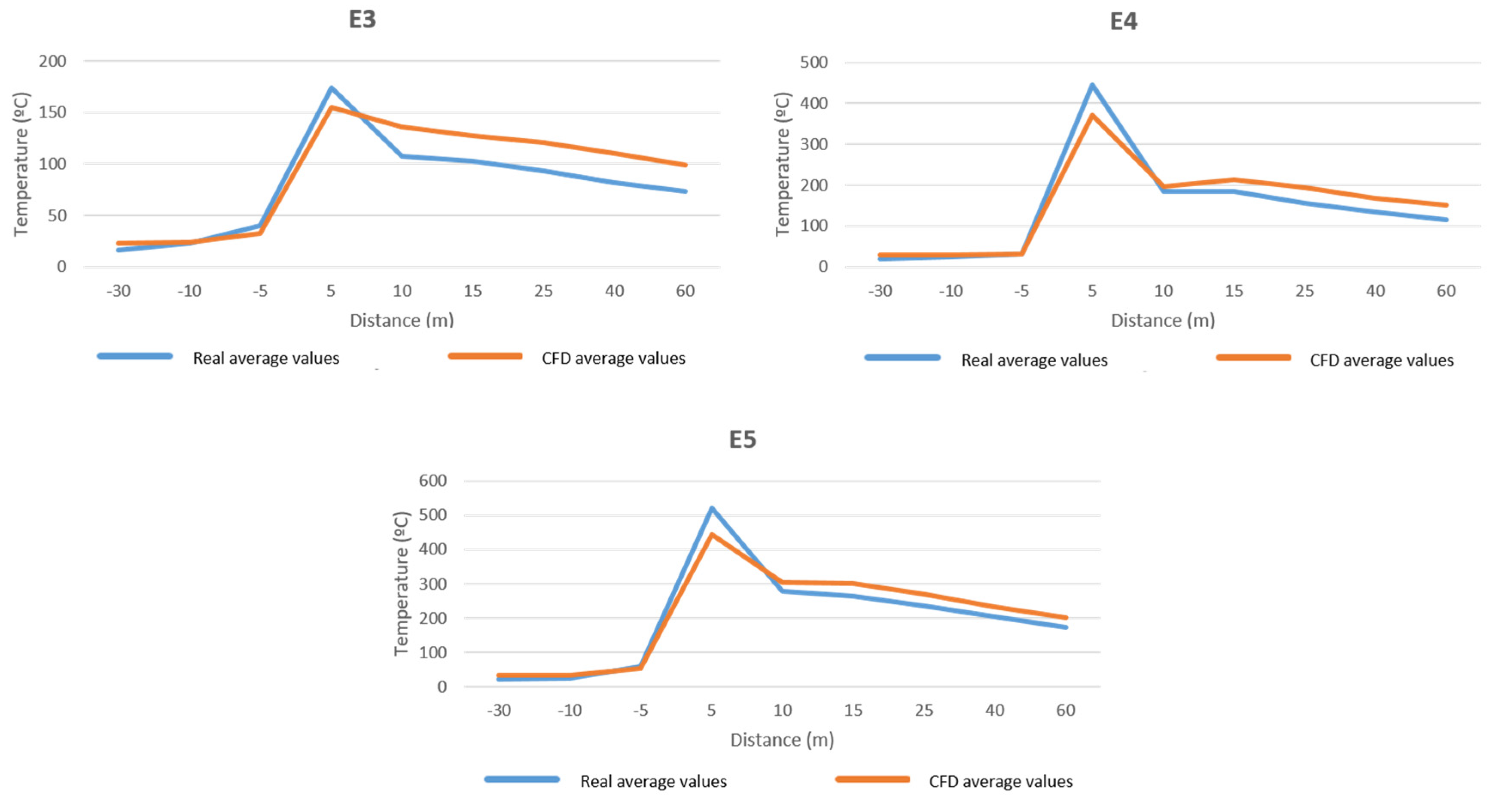
Results obtained in the experiments and the FDS model are detailed and compared below. The five scenarios depending on the fuel load and door opening are gathered in Table 5 and Table 6. As previously mentioned, there were three temperature control points at different heights in each section (P1: 2 m, P2: 1 m, P3: 0.5 m).
The mean percentage deviations between experimental and simulated values were as follows: E1, 27%; E2, 35%; E3, 24%; E4, 22%; E5, 20%. An accuracy was reached similar to other studies using CFD software to analyze the ventilation behavior in full-scale underground mine conditions [16]. The FDS simulation presented more adjustment problems with the actual values when the airflow was very low (E1 and E2). The correlation of the mean values by section between experimental data and simulations is shown in Figure 15 and Figure 16.
The FDS adjustment showed similar patterns between E1 and E2 and between E3, E4, and E5. In the first case, it showed a good experimental–FDS fit in the pre-fire zone, while the simulated values exceeded the fire temperatures in the zone after the fuel load, with a tendency to converge when the fire faded. On the other hand, trials E3, E4, and E5 showed a very good fit up to the area just after the fire, where the temperature was underestimated (S4 at 5 m) and then slightly overestimated (S5 at 10 m), following the same trend throughout the drift. Overall, the correlation between the experimental and simulated mean values was better when there was more airflow and higher firepower.
Further research stated some variations in the results with newer FDS versions [27], but consistent with experimental data in both cases [27]. Moreover, the performance and accuracy of the FDS version used in the study was validated in previous studies comparing simulations and experimental data [25], which is in accordance with the outcomes achieved in this study. Results are adequate to study fire situations in underground mining, but further research should be done to be fully applicable for tunneling and other large closed spaces, specifically increasing the accuracy of the simulations with a smaller grid cell and examining the immediate area around the fire.
4. Conclusions
The performance of the fire, as a function of time, was defined in a monitored real-scale space and subjected to distinct fire scenarios that can be extrapolated to possible fires in a mine, varying the airflow, fuel load, and door opening. These scenarios were set in terms of combustion pollutant emission, airflow fluctuation, and temperatures throughout the entire drift, either in length or at different heights, as well as the interaction of these parameters over time.
The experiments proved that an abrupt reduction in the air supply had a much greater impact on the variation of the gas concentration than an increase in the fuel load. Despite the fires following the theoretical principles, the airflow–fuel load ratio considerably varied the fire behavior over time in terms of temperature, pollutants emitted, airflow variation, and the development of the roll-back phenomenon.
In addition, several fire simulations were performed, adapting the FDS code for the five most relevant scenarios, comparing the results with the actual tests and obtaining a good correlation between simulated and experimental values. The average of the maximum deviations in all the sections was 24%, obtaining the smallest deviations in the areas near the focus of the fire and in the upper part of the drift (around 10%).
The adjusted parameters in the model can be used for future analysis of fires in other mining activities or underground spaces, especially regarding the airflow behavior and temperatures reached. Furthermore, it can be very useful to analyze and define the most efficient emergency measures or the potential impact that a fire could generate in the critical areas of the mine.
Author Contributions
Conceptualization, F.F.-A., A.M.C., and F.G.-F.; methodology, F.F.-A., A.M.C., and F.G.-F.; validation, F.F.-A., A.M.C., and F.G.-F.; formal analysis, F.F.-A., A.M.C., and M.B.; investigation, F.F.-A., A.M.C., F.G.-F., and M.B.; writing—original draft preparation, F.F.-A., A.M.C., and M.B.; writing—review and editing, F.F.-A., A.M.C., F.G.-F., and M.B. All authors have read and agreed to the published version of the manuscript.
Funding
This research was funded by the Junta de Castilla y León (Spain), project LE167G18, as well as the European Union through the programs ECSC and RFCS, grant numbers 7220-PR/061 and RFCR-CT-2010-00005.
Acknowledgments
The authors would like to thank the AITEMIN Technology Center and its research staff, especially the León Center, as well as HUNOSA and Fundación Santa Bárbara, where the experimental work was carried out.
Conflicts of Interest
The authors declare no conflicts of interest.
References
- Smith, A.C.; Thimons, E.D. Summary of US Mine Fire Research. SME Annual Meeting and Exhibit; Society for Mining, Metallurgy, and Exploration, Inc.: Englewood, CO, USA, 2010; pp. 1–15. [Google Scholar]
- Larry Grayson, R.; Kinilakodi, H.; Kecojevic, V. Pilot sample risk analysis for underground coal mine fires and explosions using MSHA citation data. Saf. Sci. 2009, 47, 1371–1378. [Google Scholar] [CrossRef]
- Sanmiquel, L.; Bascompta, M.; Anticoi, H.F. Analysis of a historical accident in a Spanish coal mine. Int. J. Environ. Res. Public Health 2019, 16, 3615. [Google Scholar] [CrossRef] [PubMed] [Green Version]
- Hansen, R. Fire behaviour of multiple fires in a mine drift with longitudinal ventilation. Int. J. Min. Sci. Technol. 2018. [Google Scholar] [CrossRef]
- Wang, S.; Li, X.; Wang, D. Mining-Induced void distribution and application in the hydro-Thermal investigation and control of an underground coal fire: A case study. Process Saf. Environ. Prot. 2016. [Google Scholar] [CrossRef]
- Prakash, A.; Vekerdy, Z. Design and implementation of a dedicated prototype GIS for coal fire investigations in North China. Int. J. Coal Geol. 2004, 59, 107–119. [Google Scholar] [CrossRef]
- NIOSH. Analysis of Mine Fires for All U.S. Metal / Nonmetal Mining Categories, 1990–2001. 2004. [Google Scholar]
- Hartman, H.L.; Mutmansky, J.M.; Wang, Y.J. Mine Ventilation and Air Conditioning, 3rd ed.; Wiley; Technology & Engineering: New York, NY, USA, 1997; ISBN 0471116351. [Google Scholar]
- McPherson, M.J. Subsurface Ventilation and Environmental Engineering; Springer Netherlands: Heidelberg, Germany, 1993; ISBN 978-94-011-1550-6. [Google Scholar]
- Bhattacharjee, S.; Roy, P.; Ghosh, S.; Misra, S.; Obaidat, M.S. Wireless sensor network-based fire detection, alarming, monitoring and prevention system for Bord-And-PILLAR coal mines. J. Syst. Softw. 2012, 85, 571–581. [Google Scholar] [CrossRef]
- Brune, J.F.; Saki, S.A. Prevention of gob ignitions and explosions in longwall mining using dynamic seals. Int. J. Min. Sci. Technol. 2017, 27, 999–1003. [Google Scholar] [CrossRef]
- Tutak, M.; Brodny, J. The impact of the strength of roof rocks on the extent of the zone with a high risk of spontaneous coal combustion for fully powered longwalls ventilated with the Y-Type system-A case study. Appl. Sci. 2019, 9, 5315. [Google Scholar] [CrossRef] [Green Version]
- Kallianiotis, A.; Kaliampakos, D. Optimization of exit location in underground spaces. Tunn. Undergr. Space Technol. 2016, 60, 96–110. [Google Scholar] [CrossRef]
- Wang, K.; Jiang, S.; Ma, X.; Wu, Z.; Shao, H.; Zhang, W.; Cui, C. Information fusion of plume control and personnel escape during the emergency rescue of external-Caused fire in a coal mine. Process Saf. Environ. Prot. 2016, 103, 46–59. [Google Scholar] [CrossRef]
- Li, G.; Hu, J.; Hao, X. Application and Research of Swirling Curtain Dust Collection Technology in Mines. Appl. Sci. 2020, 10, 2005. [Google Scholar] [CrossRef] [Green Version]
- Diego, I.; Torno, S.; Toraño, J.; Menéndez, M.; Gent, M. A practical use of CDF for ventilation of underground Works. Tunn. Undergr. Space Technol. 2011, 26, 189–200. [Google Scholar] [CrossRef]
- Guo, X.; Zhang, Q. Analytical solution, experimental data and CFD simulation for longitudinal tunnel fire ventilation. Tunn. Undergr. Space Technol. 2014, 42, 307–313. [Google Scholar] [CrossRef]
- Du, T.; Yang, D.; Ding, Y. Driving force for preventing smoke backlayering in downhill tunnel fires using forced longitudinal ventilation. Tunn. Undergr. Space Technol. 2018, 79, 76–82. [Google Scholar] [CrossRef]
- Zanzi, C.; Gómez, P.; López, J.; Hernández, J. Analysis of heat and smoke propagation and oscillatory flow through ceiling vents in a large-Scale compartment fire. Appl. Sci. 2019, 9, 3305. [Google Scholar] [CrossRef] [Green Version]
- Zhao, Y.C.; Zhu, G.Q.; Gao, Y.J.; Tao, H.J. Study on Temperature Field of Fire Smoke in Utility Tunnel with Different Cross Sections. Procedia Eng. 2018, 211, 1043–1051. [Google Scholar] [CrossRef]
- Sun, J.; Fang, Z.; Tang, Z.; Beji, T.; Merci, B. Experimental study of the effectiveness of a water system in blocking fire-induced smoke and heat in reduced-Scale tunnel tests. Tunn. Undergr. Space Technol. 2016, 56, 34–44. [Google Scholar] [CrossRef] [Green Version]
- Tong, Y.; Zhai, J.; Wang, C.; Zhou, B.; Niu, X. Possibility of using roof openings for natural ventilation in a shallow urban road tunnel. Tunn. Undergr. Space Technol. 2016, 54, 92–101. [Google Scholar] [CrossRef]
- Yuan, L.; Zhou, L.; Smith, A.C. Modeling carbon monoxide spread in underground mine fires. Appl. Therm. Eng. 2016, 100, 1319–1326. [Google Scholar] [CrossRef] [Green Version]
- Weisenpacher, P.; Glasa, J.; Halada, L. Automobile interior fire and its spread to an adjacent vehicle. J. Fire Sci. 2016, 34, 305–322. [Google Scholar] [CrossRef]
- Zalosh, R. Explosion Protection. SFPE Handbook of Fire Protection Engineering, 3th ed.; DiNenno, P.J., Ed.; NFPA: Quincy, MA, USA, 2002. [Google Scholar]
- Banerjee, S.C. A Theoretical Desing to the Determination of Risk Index of Spontaneous Fires in Coal Mines. J. Mines Metals Fuels 1982, 30, 399–406. [Google Scholar]
- Weisenpacher, P.; Glasa, J.; Sipkova, V. Performance of FDS versions 5 and 6 in passenger car fire computer simulation. In Proceedings of the 28th European Modeling and Simulation Symposium, EMSS 2016, Larnaca, Cyprus, 26–28 September 2016; pp. 155–161. [Google Scholar]
Figure 1.
Scheme of the facilities.
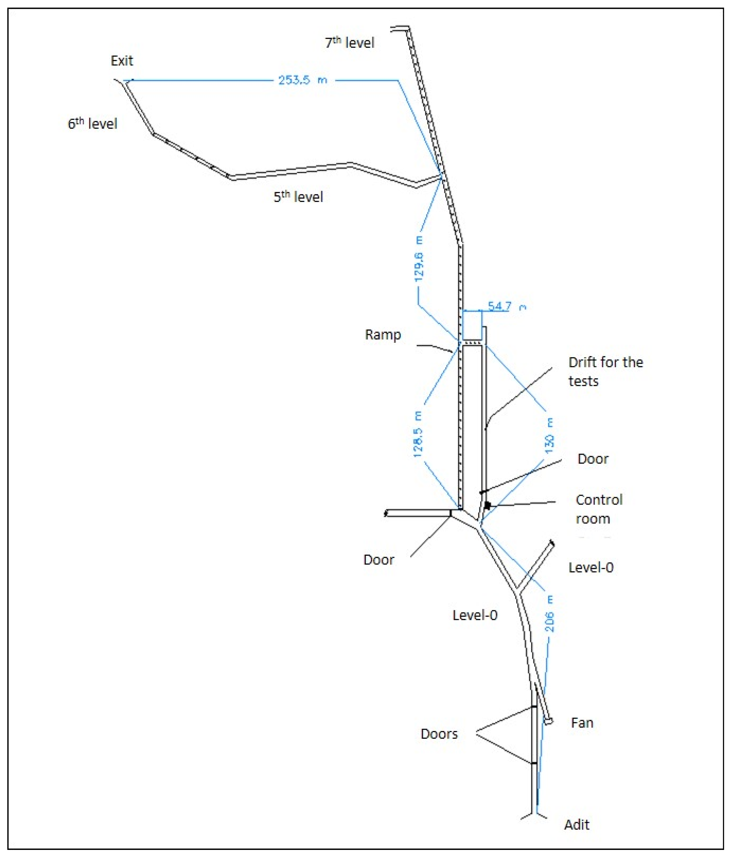
Figure 2.
Scheme of the testing drift.
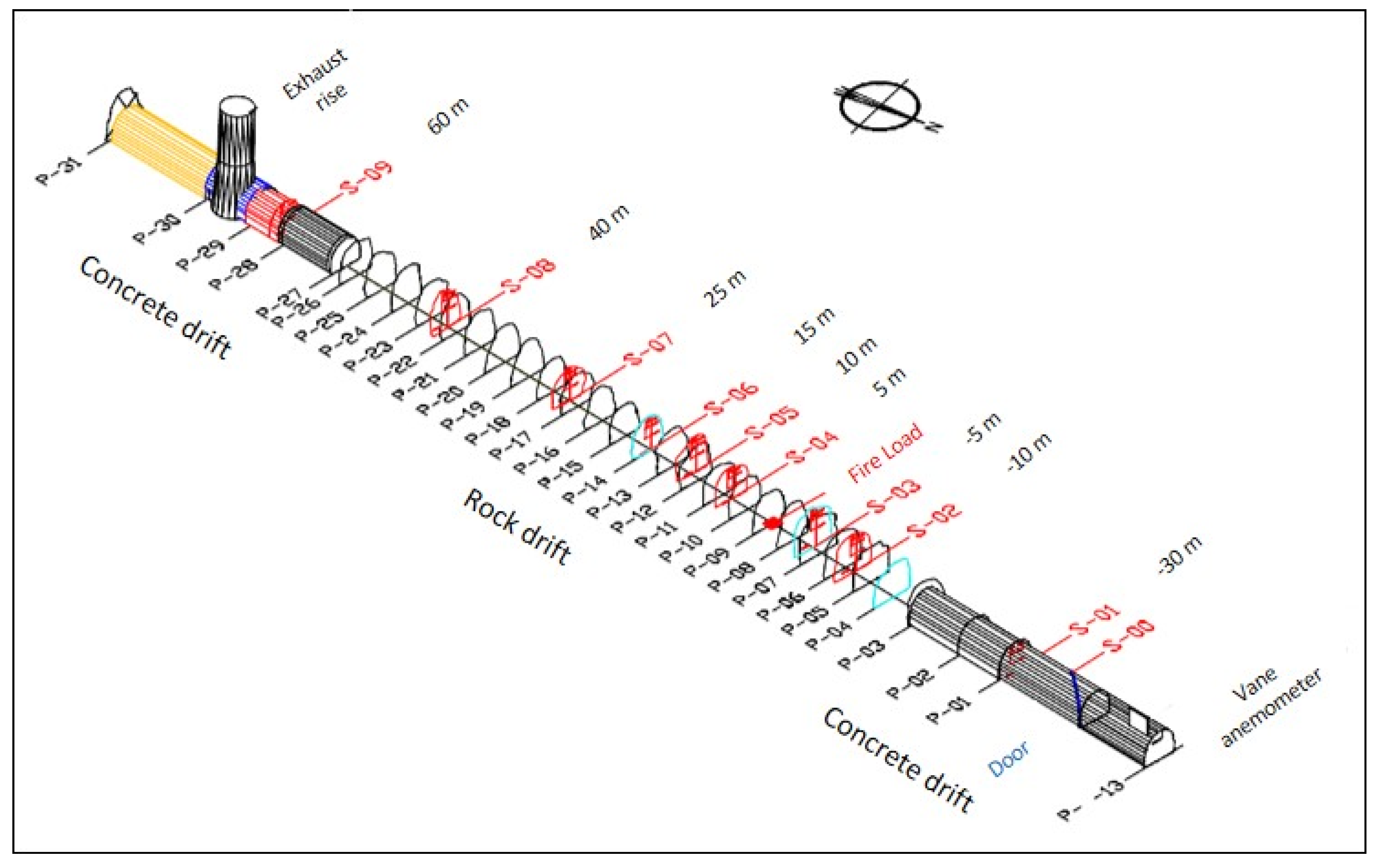
Figure 3.
Section of the testing drift with the sensors, T, at different heights.
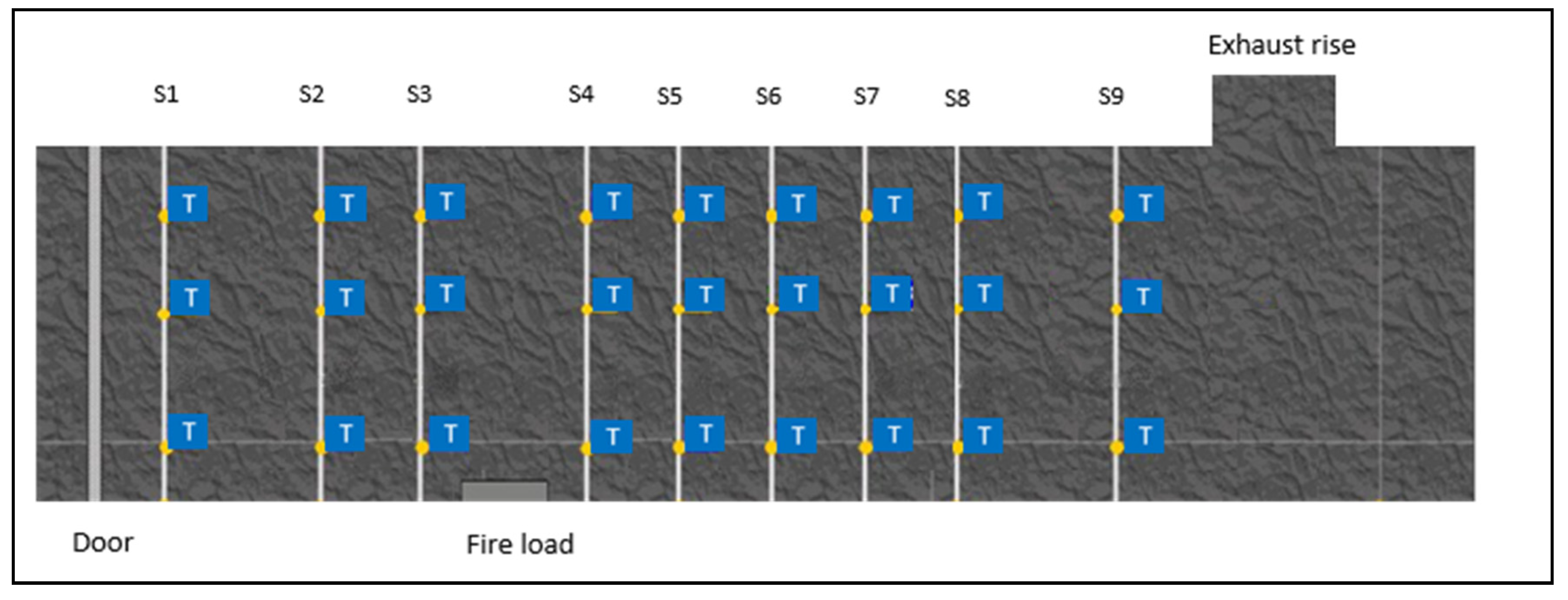
Figure 4.
XYZ meshing of the drift.
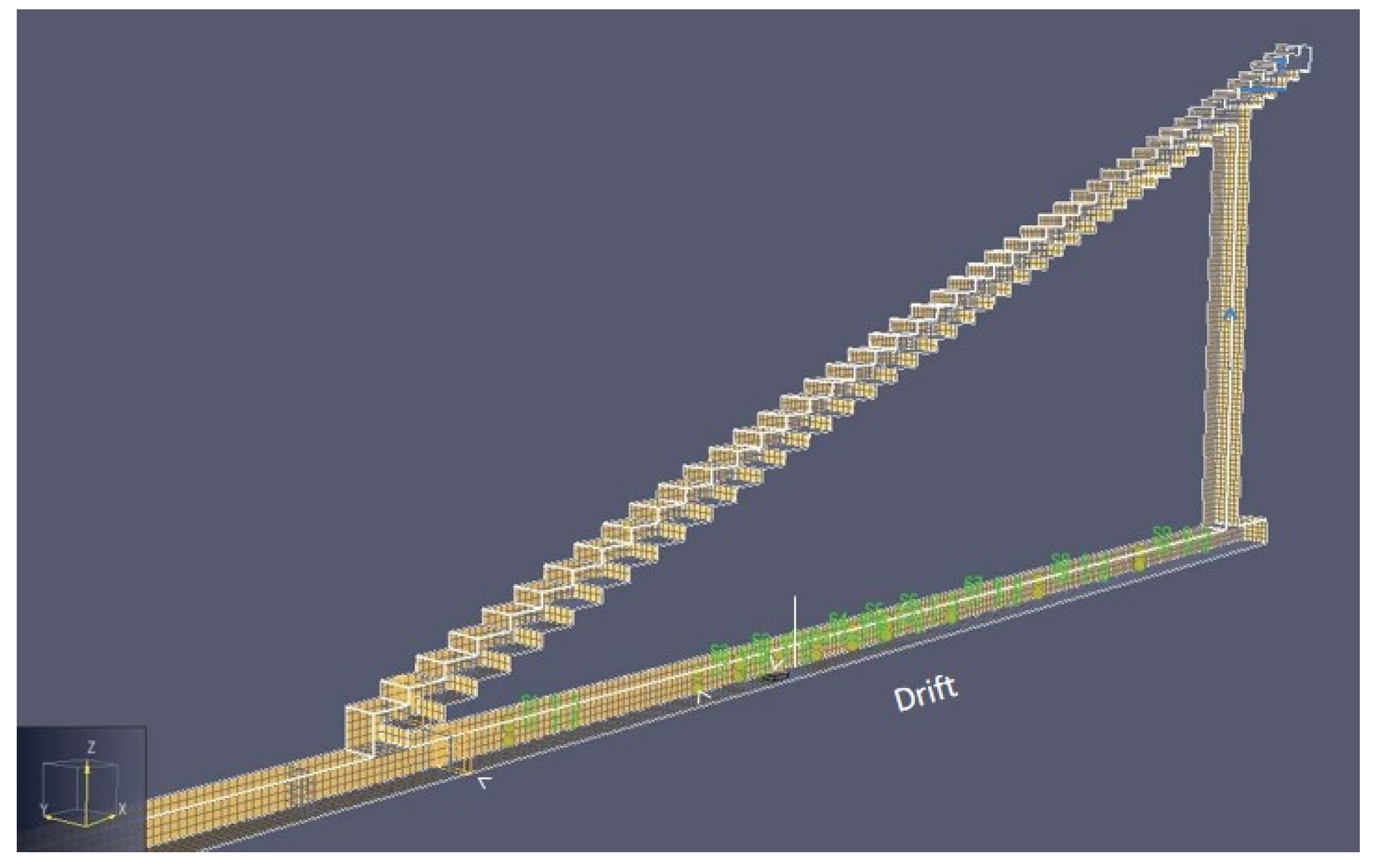
Figure 5.
Evolution of the environmental conditions over time; test 1.
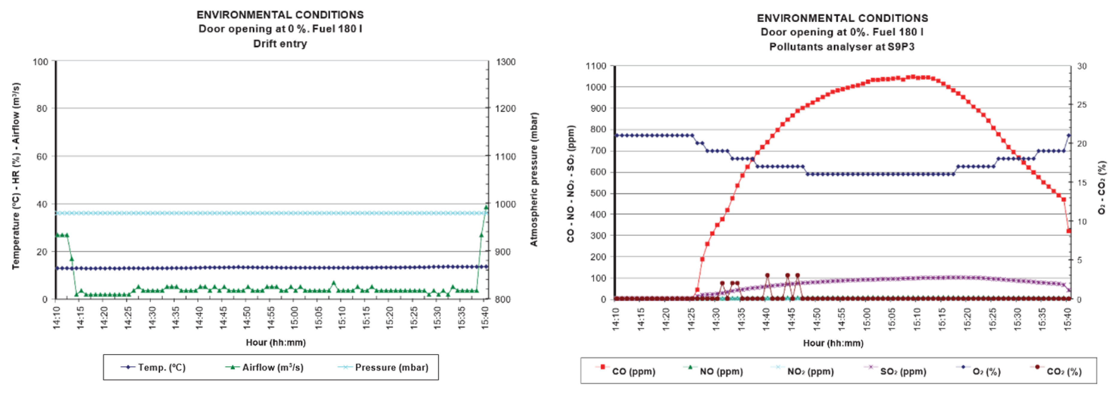
Figure 6.
Evolution of the environmental conditions over time; test 2.
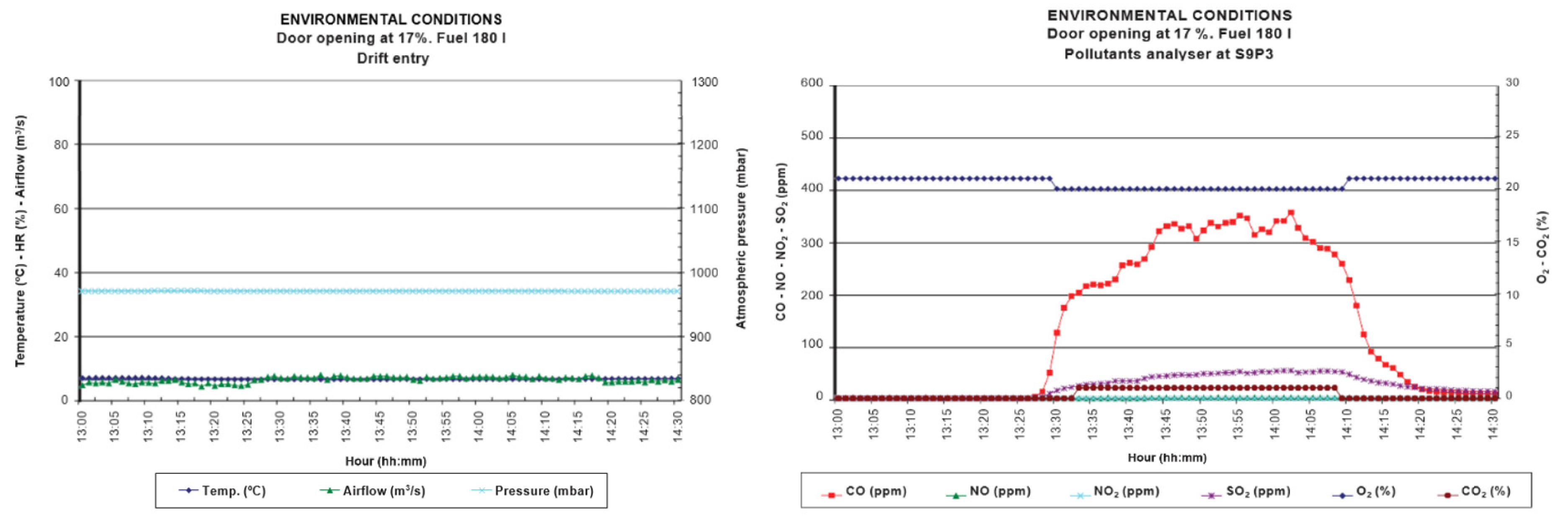
Figure 7.
Evolution of the environmental conditions over time; test 3.
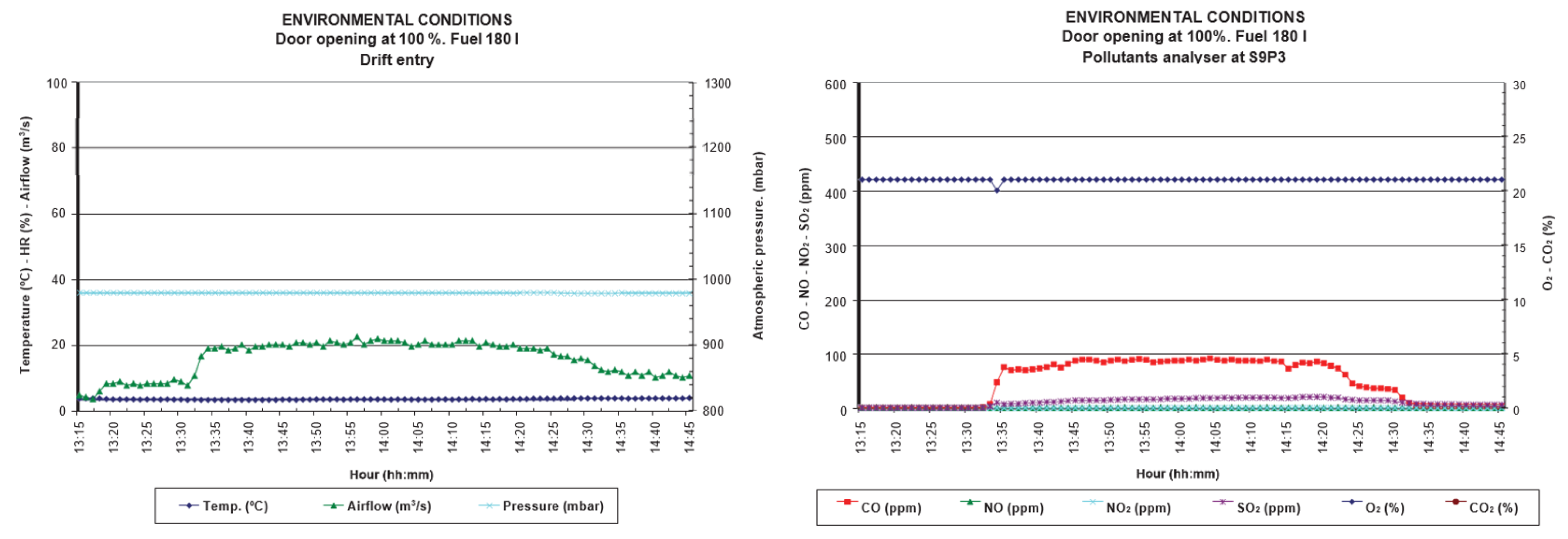
Figure 8.
EvolutioSn of the environmental conditions over time; test 4.
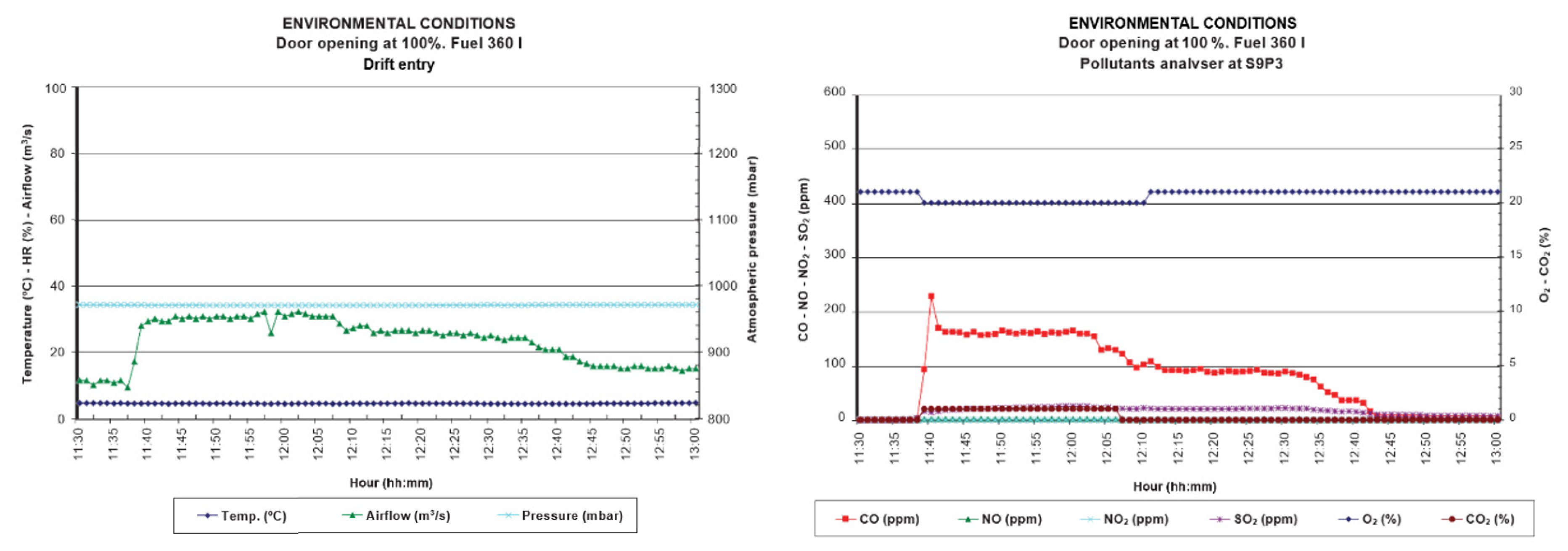
Figure 9.
Evolution of the environmental conditions over time; test 5.
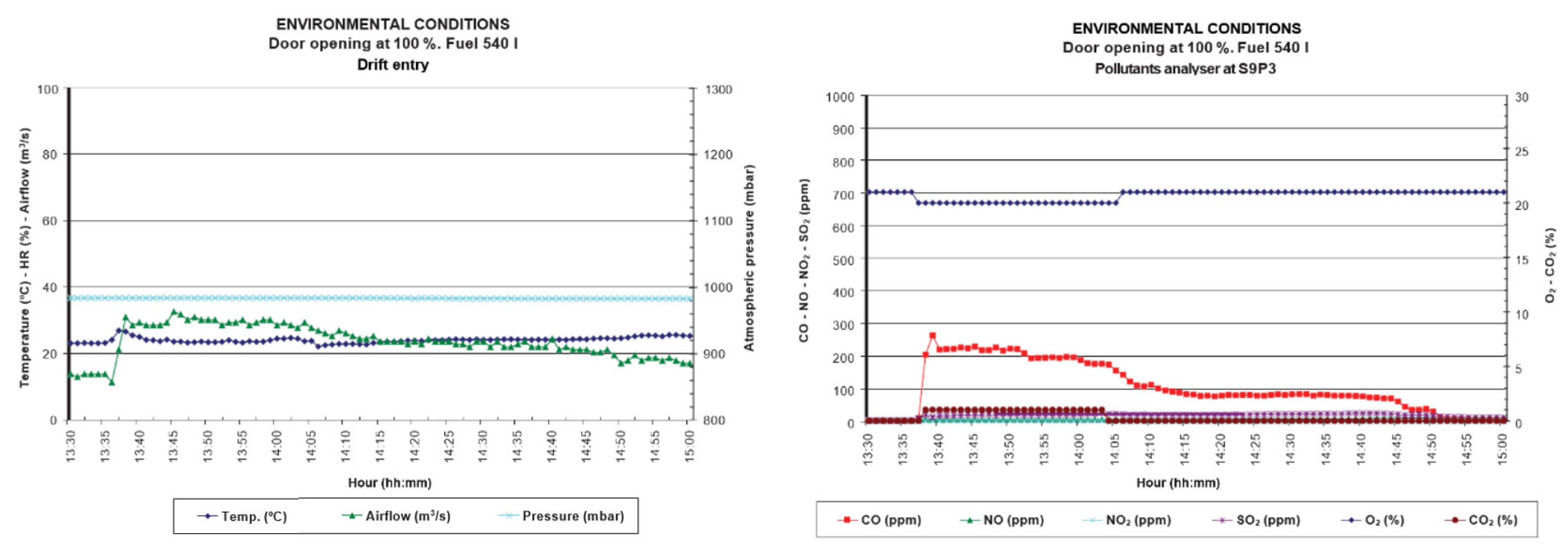
Figure 10.
Evolution of the temperature along the drift at different heights; scenario 1.
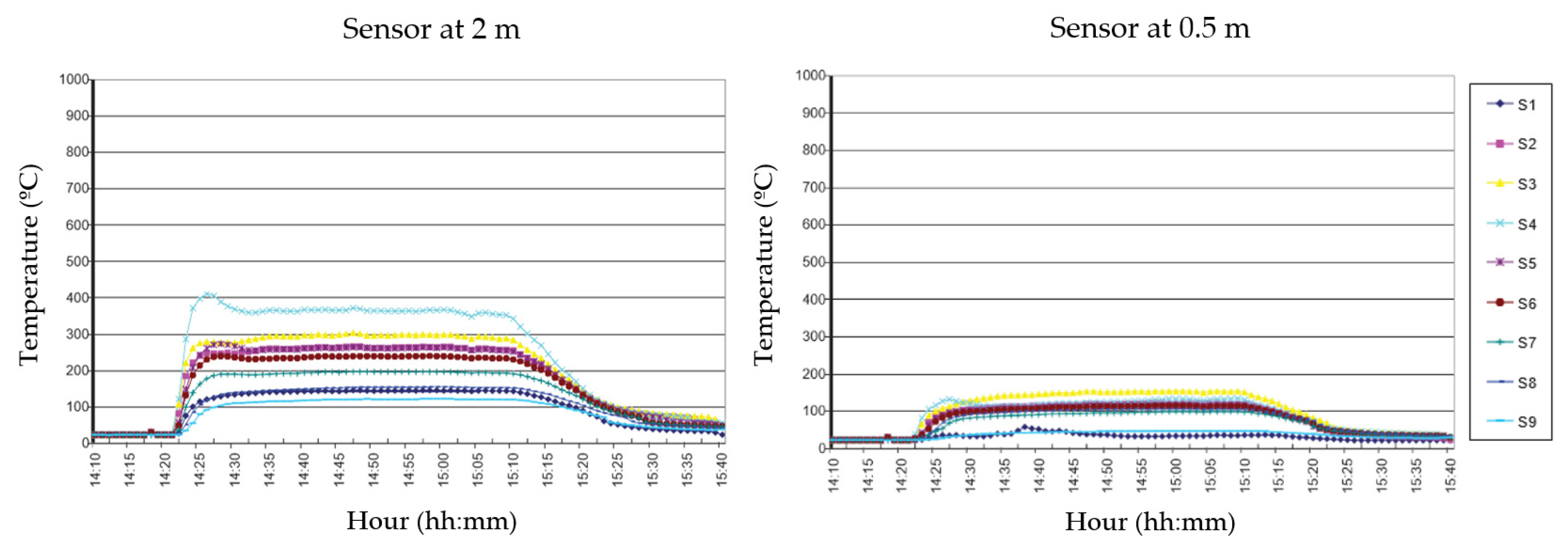
Figure 11.
Evolution of the temperature along the drift at different heights; scenario 2.
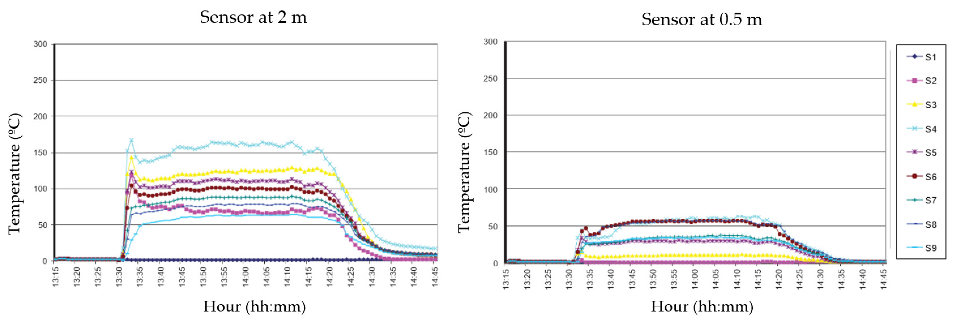
Figure 12.
Evolution of the temperature along the drift at different heights; scenario 3.
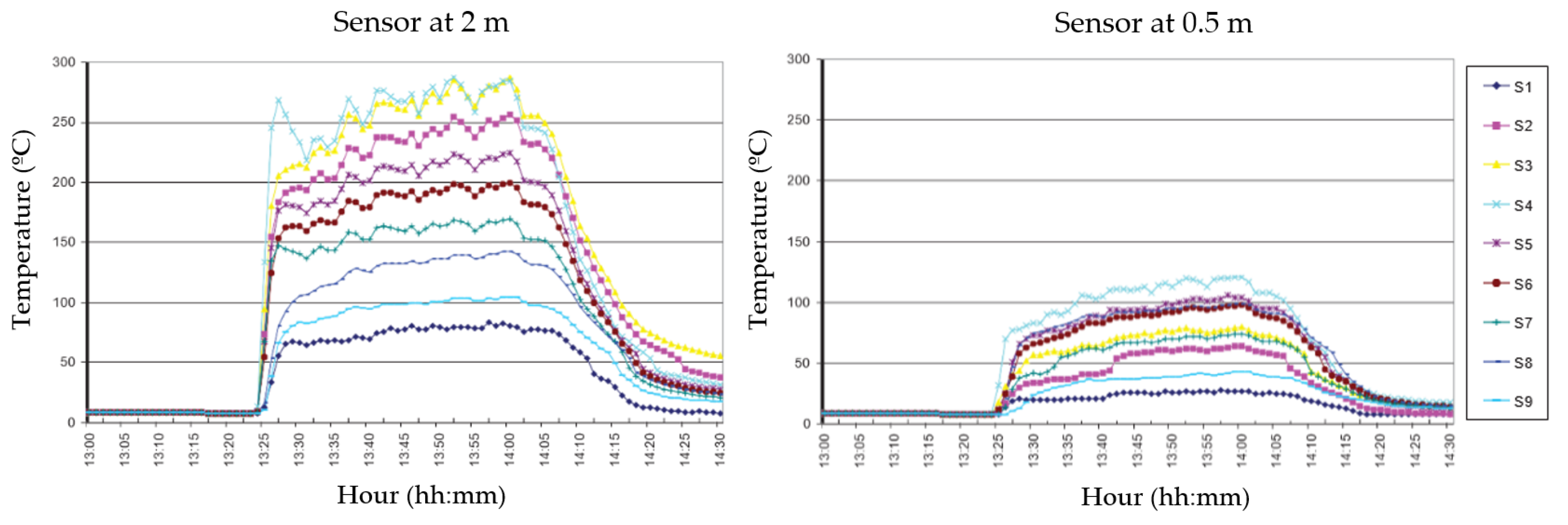
Figure 13.
Evolution of the temperature along the drift at different heights; scenario 4.
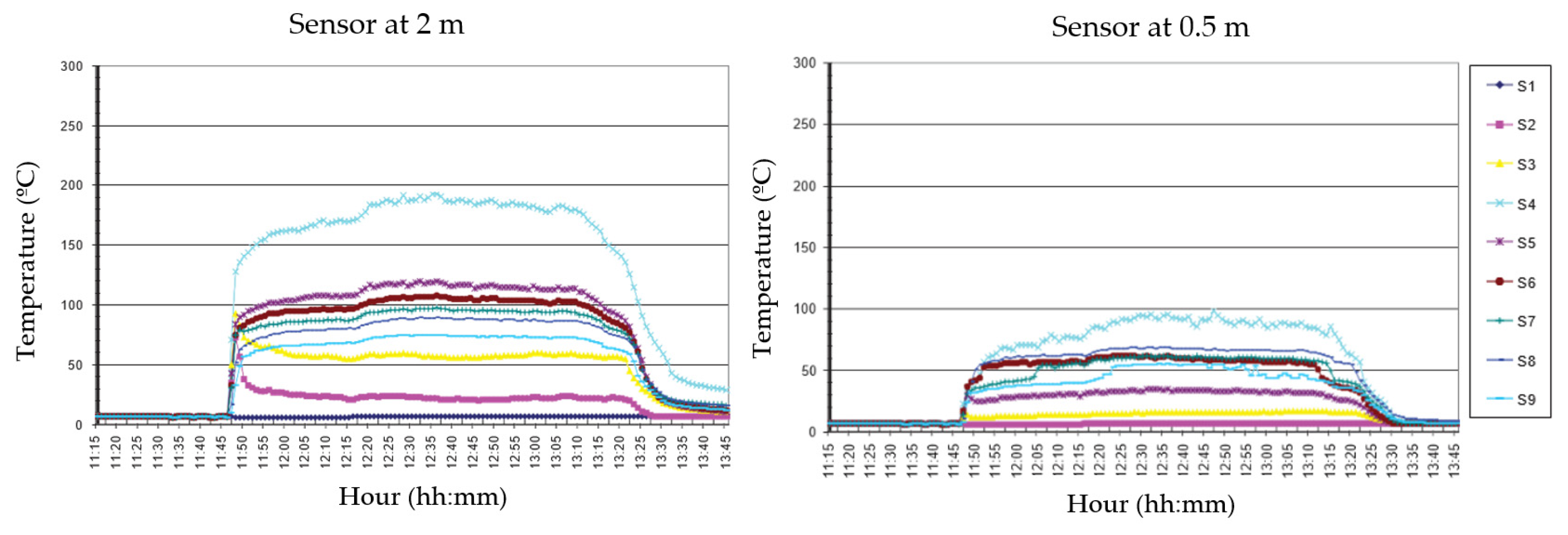
Figure 14.
Evolution of the temperature along the drift at different heights; scenario 5.
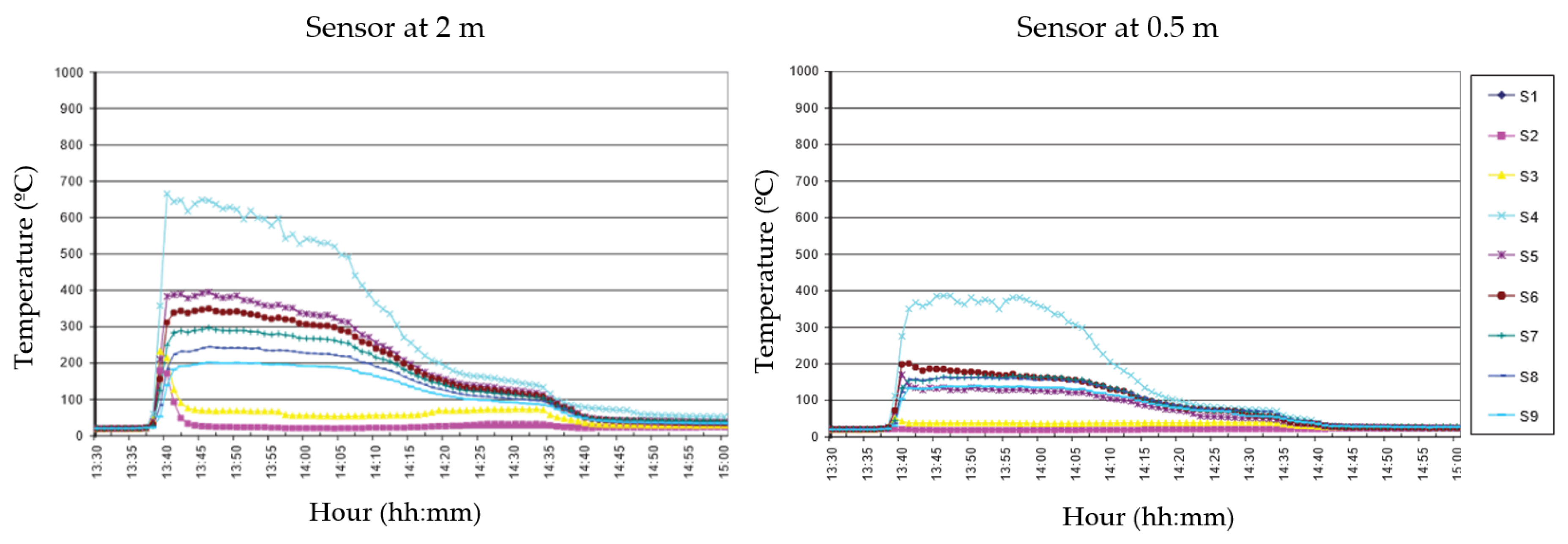
Figure 15.
Comparison of FDS and experimental temperature average values along the drift; tests E1 and E2.
Figure 15.
Comparison of FDS and experimental temperature average values along the drift; tests E1 and E2.
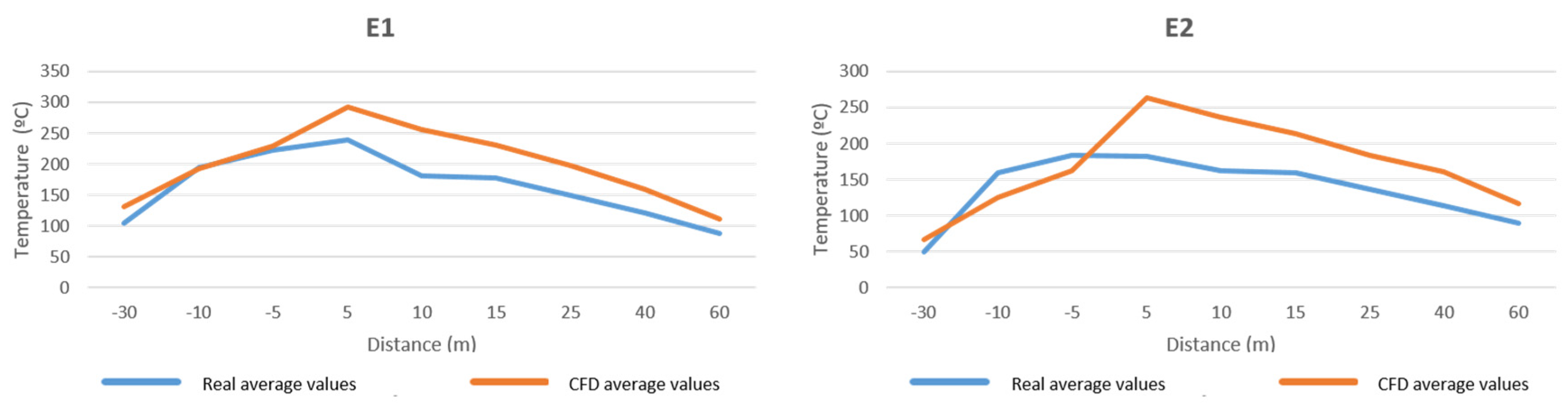
Figure 16.
Comparison FDS-Experimental temperature average values along the drift; tests E3–E5.

Table 1.
Characteristics of the sensors.
| Equipment | Type and model |
|---|---|
| Thermocouple | TC Ltd. Type K |
| Anemometer | Trolex. Vortex TX 12233 Mk |
| Barometer | Wika. FBA30WB2-900Y |
| Manometer | Testo GmbH&Co. 520 D0E10 |
| ENVIRO Multisensor | Trolex. TX6522.01.51 |
| Data acquisition system | Advantech. ADAM 5000 |
Table 2.
Values used in the different scenarios. FDS—fire dynamics simulator.
| Scenarios | Experimental Data | FDS Data | Fire Load (MW) | ||
|---|---|---|---|---|---|
| Airflow (m3/s) | Velocity (m/s) | Airflow (m3/s) | Velocity (m/s) | ||
| 1 (Door 0%) | 1.93 | 0.21 | 1.90 | 0.21 | 4.73 |
| 2 (Door 17%) | 5.10 | 0.57 | 5.30 | 0.59 | 4.73 |
| 3 (Door 100%) | 10.45 | 1.16 | 12.50 | 1.39 | 4.73 |
| 4 (Door 100%) | 11.05 | 1.23 | 12.50 | 1.39 | 9.46 |
| 5 (Door 100%) | 13.38 | 1.49 | 12.50 | 1.39 | 14.20 |
Table 3.
Modeling features.
| Stage | Features | Value |
|---|---|---|
| Modeling design | Cell size | 0.6 × 0.6 × 0.6 m |
| Cell size rate | 1 × 1 × 1 | |
| Number of cells | 14,625 | |
| Combustion parameters | Surface type | BURNER |
| HRR (heat release rate) | 2.220 kW/m2 | |
| Vessel dimensions | 1.8 × 1.2 m | |
| Material of the vessel | Steel Sheet | |
| Initial conditions | Air temperature | 10 °C |
| Humidity | 80% | |
| Fan airflow | 30 m3/s | |
| Simulation | Type of simulation | LES (large eddy simulation) |
| Total time | 4800 s | |
| Output data frames | 4800 |
Table 4.
Average values of the combustion pollutants.
| Conditions | O2 (%) | CO (ppm) | NOx (ppm) | SO2 (ppm) | CO2 (%) | |||||
|---|---|---|---|---|---|---|---|---|---|---|
| Max. | Min. | Mean | Max. | Mean | Max. | Mean | Max. | Mean | Max. | |
| 0%, 180 L | 21 | 16 | 958 | 1063 | 6 | 16 | 79 | 102 | - | 3 |
| 17%, 180 L | 20 | 21 | 234 | 362 | 2 | 5 | 24 | 64 | 1 | 2 |
| 100%, 180 L | 20 | 21 | 67 | 91 | 2 | 4 | 19 | 26 | 1 | 1 |
| 100%, 360 L | 20 | 21 | 132 | 233 | 2 | 3 | 23 | 25 | 1 | 2 |
| 100%, 540 L | 20 | 21 | 219 | 284 | 4 | 5 | 19 | 21 | 1 | 2 |
Table 5.
Experimental values from the tests.
| Section | Control Point | Temperature (°C) | ||||
|---|---|---|---|---|---|---|
| E1 | E2 | E3 | E4 | E5 | ||
| P1 | 139 | 78 | 16 | 19 | 23 | |
| S1 (−30 m) | P2 | 109 | 44 | 16 | 19 | 22 |
| P3 | 63 | 27 | 16 | 19 | 20 | |
| P1 | 255 | 241 | 32 | 26 | 27 | |
| S2 (−10 m) | P2 | 213 | 193 | 20 | 25 | 25 |
| P3 | 113 | 42 | 16 | 20 | 22 | |
| P1 | 290 | 268 | 63 | 45 | 64 | |
| S3 (−5 m) | P2 | 233 | 218 | 34 | 31 | 63 |
| P3 | 144 | 64 | 22 | 16 | 49 | |
| P1 | 355 | 264 | 212 | 502 | 593 | |
| S4 (5 m) | P2 | 244 | 181 | 184 | 503 | 590 |
| P3 | 117 | 100 | 127 | 332 | 378 | |
| P1 | 251 | 216 | 133 | 260 | 368 | |
| S5 (10 m) | P2 | 185 | 172 | 102 | 188 | 284 |
| P3 | 106 | 97 | 87 | 105 | 185 | |
| P1 | 229 | 200 | 122 | 231 | 329 | |
| S6 (15 m) | P2 | 197 | 178 | 109 | 201 | 290 |
| P3 | 104 | 98 | 78 | 119 | 176 | |
| P1 | 186 | 168 | 112 | 198 | 283 | |
| S7 (25 m) | P2 | 165 | 147 | 99 | 167 | 256 |
| P3 | 99 | 95 | 69 | 103 | 166 | |
| P1 | 143 | 134 | 97 | 163 | 238 | |
| S8 (40 m) | P2 | 126 | 118 | 88 | 144 | 214 |
| P3 | 96 | 91 | 61 | 98 | 163 | |
| P1 | 113 | 109 | 85 | 138 | 199 | |
| S9 (60 m) | P2 | 101 | 100 | 81 | 127 | 182 |
| P3 | 49 | 62 | 52 | 83 | 140 | |
Table 6.
FDS values for the same scenarios.
| Section | Control Point | Temperature (°C) | ||||
|---|---|---|---|---|---|---|
| E1 | E2 | E3 | E4 | E5 | ||
| P1 | 157 | 92 | 22 | 28 | 34 | |
| S1 (−30 m) | P2 | 145 | 68 | 23 | 30 | 35 |
| P3 | 94 | 40 | 25 | 31 | 29 | |
| P1 | 276 | 195 | 26 | 31 | 35 | |
| S2 (−10 m) | P2 | 203 | 128 | 25 | 31 | 38 |
| P3 | 98 | 51 | 20 | 25 | 32 | |
| P1 | 344 | 260 | 45 | 35 | 45 | |
| S3 (−5 m) | P2 | 237 | 175 | 30 | 38 | 51 |
| P3 | 107 | 55 | 20 | 23 | 62 | |
| P1 | 402 | 336 | 181 | 412 | 508 | |
| S4 (5 m) | P2 | 311 | 291 | 141 | 404 | 499 |
| P3 | 163 | 165 | 142 | 296 | 326 | |
| P1 | 334 | 296 | 158 | 257 | 388 | |
| S5 (10 m) | P2 | 283 | 268 | 141 | 208 | 326 |
| P3 | 150 | 144 | 108 | 126 | 200 | |
| P1 | 289 | 261 | 149 | 248 | 350 | |
| S6 (15 m) | P2 | 254 | 241 | 142 | 227 | 328 |
| P3 | 149 | 139 | 89 | 163 | 224 | |
| P1 | 235 | 218 | 139 | 224 | 313 | |
| S7 (25 m) | P2 | 216 | 205 | 140 | 223 | 303 |
| P3 | 140 | 127 | 83 | 136 | 196 | |
| P1 | 182 | 184 | 120 | 186 | 258 | |
| S8 (40 m) | P2 | 173 | 169 | 121 | 185 | 258 |
| P3 | 121 | 130 | 88 | 136 | 184 | |
| P1 | 136 | 145 | 103 | 158 | 213 | |
| S9 (60 m) | P2 | 132 | 134 | 107 | 164 | 220 |
| P3 | 64 | 71 | 86 | 129 | 172 | |
© 2020 by the authors. Licensee MDPI, Basel, Switzerland. This article is an open access article distributed under the terms and conditions of the Creative Commons Attribution (CC BY) license (http://creativecommons.org/licenses/by/4.0/).
Share and Cite
MDPI and ACS Style
Fernández-Alaiz, F.; Castañón, A.M.; Gómez-Fernández, F.; Bascompta, M. Mine Fire Behavior under Different Ventilation Conditions: Real-Scale Tests and CFD Modeling. Appl. Sci. 2020, 10, 3380. https://doi.org/10.3390/app10103380
AMA Style
Fernández-Alaiz F, Castañón AM, Gómez-Fernández F, Bascompta M. Mine Fire Behavior under Different Ventilation Conditions: Real-Scale Tests and CFD Modeling. Applied Sciences. 2020; 10(10):3380. https://doi.org/10.3390/app10103380
Chicago/Turabian StyleFernández-Alaiz, Florencio, Ana Maria Castañón, Fernando Gómez-Fernández, and Marc Bascompta. 2020. "Mine Fire Behavior under Different Ventilation Conditions: Real-Scale Tests and CFD Modeling" Applied Sciences 10, no. 10: 3380. https://doi.org/10.3390/app10103380
Note that from the first issue of 2016, this journal uses article numbers instead of page numbers. See further details here.