Peeling Damage Recognition Method for Corn Ear Harvest Using RGB Image

Abstract

Corn ear damage caused by peeling significantly influence the output and quality of corn harvest. Ear damage recognition is the basis to adjust working parameters and to reduce damage. Image processing is attracting increasing attentions in the field of agriculture. Conventional image processing methods are difficult to be used for recognizing corn ear damage caused by peeling in field harvesting. To address the this problem, in this paper, we propose a peeling damage recognition method based on RGB image. For our method, we develop a dictionary-learning-based method to recognize corn kernels and a thresholding method to recognize ear damage regions. To obtain better performance, we also develop the corroding algorithm and the expanding algorithm for the post-processing of recognized results. The experimental results demonstrate the practicality and accuracy of the proposed method. This study could provide the theoretical basis to develop online peeling damage detection system for corn ear harvesters.

1. Introduction

Corn is one of the largest crops grown around the world due to its application in food, feed, chemical engineering, and energy [1,2,3]. Mechanization and automation for corn harvest have been fully developed in the last century. In America, Oceania, and Europe, corn kernels are usually obtained directly through harvest process using grain harvesters or combined grain-stover harvesters [4]. However, for some growing regions in Asia, the moisture is too large for kernel harvest, as it would induce unacceptable kernel damage [5]. Hence, the segmented harvesting is widely applied in such regions [6]. Specifically, corn ears are snapped firstly in the farmland by a harvester, as shown in Figure 1a. Then, corn ears are dried until the moisture content of kernels are suitable for threshing. However, as shown in Figure 1b, corn ears are inevitably damaged by the peeling devices. Ear damage means the corn kernels drop from ears during the peeling process, and the dropped kernels fail to be harvested, leading to considerable harvest loss. Preliminary studies have demonstrated corn ear damage is mainly affected by the rotation speed, surface structure, and material and installation clearance of snapping roller and transmission blade [7,8]. Researchers believe adjusting these working parameters can effectively reduce corn ear damage [9,10]. However, the adjusting operation cannot be executed without efficient and accurate recognition of corn ear damage. In other words, recognition is the technical prerequisite to reduce damage. Therefore, it is necessary to develop an automatic, non-contact, non-destructive, and rapid method for corn ear damage recognition.

Image processing methods have been attracting increasing attentions in agriculture products non-destructive detection [11,12]. Depending on the type of information, such methods can be divided into hyperspectral image (HSI) processing methods and nature image processing methods [13,14]. HSIs comprise dozens or hundreds of narrow spectral bands with high spatial resolution, such that they are able to be used for recognition of objects [14]. Due to its great volume and high cost, HSI recognition is frequently employed for agriculture products detection in post-harvest. For instance, Atas et al. developed a compact machine vision system to detect aflatoxin in chilli peppers based on HSIs and machine learning [15]. Farrell et al. utilized HSIs to identify water and nitrogen availability for rainfed corn crops [16]. Nature images are acquired by normal camera [17,18,19]. RGB images are the typical form of nature images [20,21]. Comparing to HSIs, RGB images are more suitable for online agricultural detection as its lower computational complexity and cost. For the field of seeding, Leemans et al. developed a machine-vision-based mechanism to measure position of seed drills relative to the previous lines, which is used in a feedback control loop [22]. Karayel et al. utilized high-speed camera system to measure the seed drill seed spacing and velocity of fall of seeds [23]. Liu et al. proposed an image processing algorithm to detect the performance of seed-sowing devices, including the the breadth of the seed array, the coordinates of the seed array center, the distance between seed arrays, and seed intervals and non-seed intervals of each seed array [24]. For the filed of harvesting, Gunchenko et al. used unmanned aerial vehicle to acquire nature images for agricultural harvesting equipment route planning and harvest volume measuring [25]. Plebe et al. developed an image processing system to guide automatic harvesting of oranges [26]. Jia et. al proposed an image preprocessing method for night vision of apple harvesting robot [27].

For the field of corn ear harvest, damage forms are various in different processes, such as whole ear broken, kernel damage, and peeling ear damage. In ear snapping process, a whole ear may be broken off by headers. To address this issue, Liu et al. employed a camera to acquire RGB images of ears on conveyor belt, and then proposed a method to distinguish broken ear based on YOLO [6]. The information of ear broken can be used to adjust header speed. Kernel damage is also attracting research interests, which means kernels are cracked during harvesting. Liao et al. utilized on-board hardware operation and parallel statistical look-up table mapping to extract images of kernels, based on which the image processing algorithm is developed to distinguish whole and damaged kernels [28]. Another damage form is ear peeling damage, the primary characteristic of which is the kernel loss from ears. Unfortunately, to date, the automatic detection of ear peeling damage has not been reported.

The recognition method is the basis of online detection of ear peeling damage. Mechanical peeling leads to random dropping of kernels from ears. Hence, comparing to kernel damage, ear damage usually exhibits large region and random distribution. These characteristics make it necessary and possible to be recognized by RGB images. However, conventional image processing methods, such as image segmentation [29,30], are difficult to be applied to recognize the damage in corn ear. This is because the objective images of snapped ears always contain great amount of features. Next, we provide an example to illustrate this issue. As presented in Figure 2a, we selected a typical objective image during snapping as the original image in this example with the spatial resolution of $700\times 700$, containing intact ears, damaged ears, impurities, and backgrounds. The well-known image segmentation method, thresholding, was used for the objective image [31,32,33,34]. The red, green, and blue bands were employed for the test, respectively. The result is shown in Figure 2. The image is divided into numerous of parts, and the region of damage is almost impossible to be recognized, regardless of the used band.

In this study, we aimed to develop a peeling damage recognition method based on RGB image. Different from conventional methods, the proposed method contains two steps. First, we recognize the regions of corn kernels by using a novel dictionary-learning-based method. Second, we recognize the ear damage in the regions outside of the kernel regions by using a novel thresholding method. For both two steps, we also develop the method based on the concept of image corrosion and expansion for post-processing of recognized results. The practicality and accuracy of the proposed method was verified through experiments on both single ear recognition and multiple ears recognition. This paper is organized as follows. Section 2 introduces the the materials used in this study and the methods to recognize corn kernel region and ear damage region. Section 3 and Section 4 presents the experimental results and discussions, respectively. Section 5 concludes this paper.

2. Materials and Methods

In this section, we first introduce the materials used in this study. Next, we introduce the proposed recognition method, including recognition of corn kernel and recognition of ear damage.

2.1. Materials

The variety of used corns were Feitian 358, and they were harvested in Lishu city, Jilin province, China, which is located at ${43}^{\circ }$N and ${123}^{\circ }$E. The row spacing and the plant spacing were 600 and 269 mm, respectively. The moisture content while harvesting was 27.3%. In this producing region, more than 90% of corn is segmentally harvested. The most widely used machineries are JIMIG-562 type of harvesters. The rotation speeds of snapping roller and transmission blade were set to 370 and 120 rpm, respectively.

2.2. Recognition of Corn Kernel

In this section, we introduce the process of recognizing corn kernels that is achieved by using the correlation between the original image and the learned dictionary [35]. For this purpose, we should first train dictionaries for corn kernel, ear damage, and backgrounds. The outline of the proposed dictionary learning strategy in given in Algorithm 1. Without loss of generality, we primarily introduce the training process for corn kernels, and the methods for ear damage and backgrounds are similar. In this method, we employ a set of regions of corn kernels, containing $3\times {10}^5$ spatial pixels totally. Then, we reshape and normalize them into training samples. Figure 3 shows the graphical representation for the generation of kernel training samples. Specifically, let $\mathit{Z}\in {\mathcal{R}}^{3\times \xi }$ denote the normalized collection of selected samples, $\mathit{Z}=[{\mathit{z}}_1,{\mathit{z}}_2,\cdots ,{\mathit{z}}_{\xi }]$, and $\parallel {\mathit{z}}_t{\parallel }_2=1$, $t=1,2,\cdots ,\xi$. Each column of $\mathit{Z}$ denotes a sample, expressed as ${\mathit{z}}_t\in {\mathcal{R}}^3={[z_t^r,z_t^g,z_t^b]}^T$, where $z_t^r$, $z_t^g$, and $z_t^b$ represent the reflection of the pixel in the red, green, and blue bands, respectively. These samples are used to train a dictionary, ${\mathit{D}}^k\in {\mathcal{R}}^{3\times q}$, that satisfies

$$\begin{array}{c}\hfill \forall t\in \{1,2,\cdots ,\xi \},\parallel {{\mathit{D}}^k}^T{\mathit{z}}_t{\parallel }_{\infty }\ge ϵ,\end{array}$$

(1)

where ${\parallel ·\parallel }_{\infty }$ returns the maximum absolute entry of a vector. The above constraint ensures at least one atom of the learned dictionary is correlative enough to each sample. The parameter $ϵ$ controls the threshold of correlation. In this study, we set $ϵ=0.01$.

Algorithm 1 Proposed dictionary learning algorithm.

Require:$\mathit{Z}=[{\mathit{z}}_1,{\mathit{z}}_2,\cdots ,{\mathit{z}}_{\xi }]$, $\parallel {\mathit{z}}_t{\parallel }_2=1$, $t=1,2,\cdots ,\xi$, threshold $ϵ$.  1: Initialize $\mathit{D}=\left[\right]$;  2: for $t=1$ to $\xi$ do  3:  if $1-\parallel {\mathit{D}}^T{\mathit{z}}_t{\parallel }_{\infty }<ϵ$ then  4:  $\mathit{D}=[\mathit{D},{\mathit{z}}_t]$;  5: end if  6: end for Ensure: Learned dictionary $\mathit{D}$.

The RGB information in the objective is regarded to be similar to that in the training samples. Therefore, we can always find an atom strongly correlative to RGB data of a core kernel pixel in objective images. Besides corn kernel, we also utilize the proposed algorithm to train dictionaries for ear damage and backgrounds, denoted as ${\mathit{D}}^e$ and ${\mathit{D}}^u$, respectively. Based this consideration, we recognize whether an arbitrary spatial pixel belongs to core kernel using Algorithm 2.

Algorithm 2 Recognizing corn kernels using learned dictionaries.

Require: Original RGB image $\mathit{X}\in {\mathcal{R}}^{n_1\times n_2\times 3}$, dictionaries ${\mathit{D}}^k$, ${\mathit{D}}^e$, and ${\mathit{D}}^u$ threshold $\beta$, ${\gamma }^r$.   1: Initialize ${\mathit{C}}_1=\mathit{0}\in {\mathcal{R}}^{n_1\times n_2}$   2: for each spatial pixel $(i,j)$ do   3: Denote $\mathit{x}=\mathit{X}(i,j,:)=\mathit{x}={[x^r,x^g,x^b]}^T$,;   4: if ${\parallel \mathit{x}\parallel }_2>\beta$ and $x^r>{\gamma }^r$ then   5:  Normalize $\mathit{x}$ by ${\mathit{x}}_0=\mathit{x}/{\parallel \mathit{x}\parallel }_2$;   6:  Compute ${\mathit{p}}^k={{\mathit{D}}^k}^T{\mathit{x}}_0$, ${\mathit{p}}^e={{\mathit{D}}^e}^T{\mathit{x}}_0$, and ${\mathit{p}}^u={{\mathit{D}}^u}^T{\mathit{x}}_0$;   7:  Compute ${\alpha }^k={\parallel {\mathit{p}}^k\parallel }_{\infty }$, ${\alpha }^e={\parallel {\mathit{p}}^e\parallel }_{\infty }$, and ${\alpha }^u={\parallel {\mathit{p}}^u\parallel }_{\infty }$;   8:  if ${\alpha }^k=max\{{\alpha }^k,{\alpha }^e,{\alpha }^u\}$ then   9:   ${\mathit{C}}_1(i,j)=1$; 10:  end if 11: end if 12: end for Ensure: Recognizing result ${\mathit{C}}_1$.

We compute the correlation between ${\mathit{x}}_0$ and each atom of the dictionary and find the atom that is most correlative to ${\mathit{x}}_0$. If the atom belongs to ${\mathit{D}}^k$ and the reflection of the red band satisfies $x^r>{\gamma }^r$, we then regard this pixel as corn kernel. As indicated in Step 4 of Algorithm 2, two preconditions are set to determine whether a pixel should be an alternative based on the prior information of corn kernels. The two preconditions can reduce the interference of dark backgrounds, shadow, etc. Through the above operations, the original RGB image is transformed into binary image, ${\mathit{C}}_1$. The recognized kernels are displayed as 1, i.e., white, while other pixels are set to be 0, i.e., black.

Next, we provide an example for the proposed corn kernel recognition method. As presented in Figure 4a, a damaged ear was selected with the spatial size of $800\times 600$ for our test. The dictionary was trained using the method given in Algorithm 1 based on $3\times {10}^5$ training samples. Then, we utilized Algorithm 2 to recognize corn kernels. The results is shown in Figure 4b. Obviously, the region of kernels in Figure 4a is highly consistent with the white region in Figure 4b.

Remark 1.

It should be noted we only use Algorithm 2 to recognize corn kernels rather than ear damages. This is because ear damage is close to kernel gap in terms of RGB information, such that it is easy to confuse with damages with gap. Hence, we first recognize kernels, and then occupy the region of kernels and their gap using corroding and expanding operations. Finally, we find the damage based on RGB information within the region that is not occupied.

2.3. Recognition of Ear Damage

Corroding is used to eliminate outliers, which can also be regarded as noise. In this method, corroding is executed before expanding to avoid unexpected expansion caused by outliers. Here, we should provide the definition of the operator $\delta (·)$ in advance.

Definition 1.

Given a binary image $\mathit{C}$, the operation $\delta (·)$ with respect to a pixel $\mathit{C}$, denoted as $\delta \left(\mathit{C}\right(i,j\left)\right)$, is defined by

$$\begin{array}{c}\hfill \delta \left(\mathit{C}(i,j)\right)=\left[\sum _{a=i-1}^{i+1}\sum _{b=j-1}^{j+1}\mathit{C}(a,b)\right]-\mathit{C}(i,j).\end{array}$$

(2)

and we define $\mathit{C}(i,j)=0$ once $i=0$ or $j=0$.

Remark 2.

In fact, the operation $\delta \left(\mathit{C}\right(i,j\left)\right)$ returns the number of 1-value pixels, i.e., the number of white pixels, among its surrounding 8 pixels. However, when a pixel is located at the edge of an image, the total number of surrounding pixels is 5; when a pixel is located ing the corner, the total number of surrounding pixels is 3.

Algorithm 3 Proposed corroding algorithm.

Require: Binary image ${\mathit{C}}_1\in {\mathcal{R}}^{n_1\times n_2}$, threshold $\lambda$, maximum number of iterative cycles $t_{max}$.  1: while termination condition is not reached do  2: Initialize ${\mathit{C}}_2=\mathit{0}\in {\mathcal{R}}^{n_1\times n_2}$;  3: for each pixel ${\mathit{C}}_1(i,j)$ do  4:  if $\delta \left({\mathit{C}}_1(i,j)\right)>\lambda$ then  5:   ${\mathit{C}}_2(i,j)=1$;  6:  end if  7: end for  8: ${\mathit{C}}_1\leftarrow {\mathit{C}}_2$;  9: end while Ensure: Corroded binary image ${\mathit{C}}_2$.

The proposed corroding algorithm is summarized in Algorithm 3. Our strategy is setting a pixel to be 1 only when more than $\lambda$ of its surrounding pixels are 1. The corroding process is repeated until one of the two termination conditions is reached. The first condition is the number of iterative cycles is enough. The second is the outputted image no longer changes. The parameter $\lambda$ controls the threshold for corroding a pixel. A larger $\lambda$ encourages radical corrosion, whereas a smaller $\lambda$ leads conservative corrosion. A graphical demonstration for comparing corroding operations based on different values of $\lambda$ is provided in Figure 5. We randomly selected a patch of a binarized corn kernel image as the test image. The maximum number of iterative cycles was set to 5. Obviously, the outliers still remain after corroding when $\lambda =1$. On the other hand, too many features of kernels are corroded when $\lambda =5$. When $\lambda =3$, the outliers can be removed and the main features of kernels still exist. Therefore, we empirically set $\lambda =3$ in this study. Experimental results on the test ear are provided in Figure 6. Figure 6a shows the binary image after the kernel recognition process, which is just the image presented in Figure 4b. Figure 6b is the corroded image of Figure 6a. It is obvious most outliers have been successfully removed, and the main features of kernel are unaffected.

Next, we expand the corroded image to fill pores and gap of kernels. The proposed expanding algorithm is summarized in Algorithm 4. For each pixel, all 8 of its surrounding pixels are set to 1 if more than $\rho$ of its surrounding pixels are 1. Similar to the corroding algorithm, the total numbers of surrounding pixels for pixels at edges and corners are 5 and 3, respectively. The parameter $\rho$ controls the threshold of expanding. A smaller $\rho$ can speed up expanding. In this study, we empirically set $\rho =4$. Two termination conditions are detected after each iterative cycle, namely whether the number of iterative cycles is enough and whether the outputted image no longer changes.

Algorithm 4 Proposed expanding algorithm,

Require: Binary image ${\mathit{C}}_2\in {\mathcal{R}}^{n_1\times n_2}$, threshold $\rho$, maximum number of iterative cycles $t_{max}$.  1: while termination condition is not reached do  2: Initialize ${\mathit{C}}_3=\mathit{0}\in {\mathcal{R}}^{n_1\times n_2}$;  3: for each pixel ${\mathit{C}}_2(i,j)$ do  4:  if $\delta \left({\mathit{C}}_2(i,j)\right)>\rho$ then  5:   Set all its surrounding pixels to 1;  6:  end if  7: end for  8: ${\mathit{C}}_2\leftarrow {\mathit{C}}_3$;  9: end while Ensure: Expanded binary image ${\mathit{C}}_3$.

The expanded result of the corroded image is presented in Figure 6c. Comparing the corroded image, i.e., Figure 6b, the pores and gap get apparent filling. Using the corrosion and expanding operations, we can not only accurately determine the region of kernels, but also reduce the searching scope for the following damage recognition.

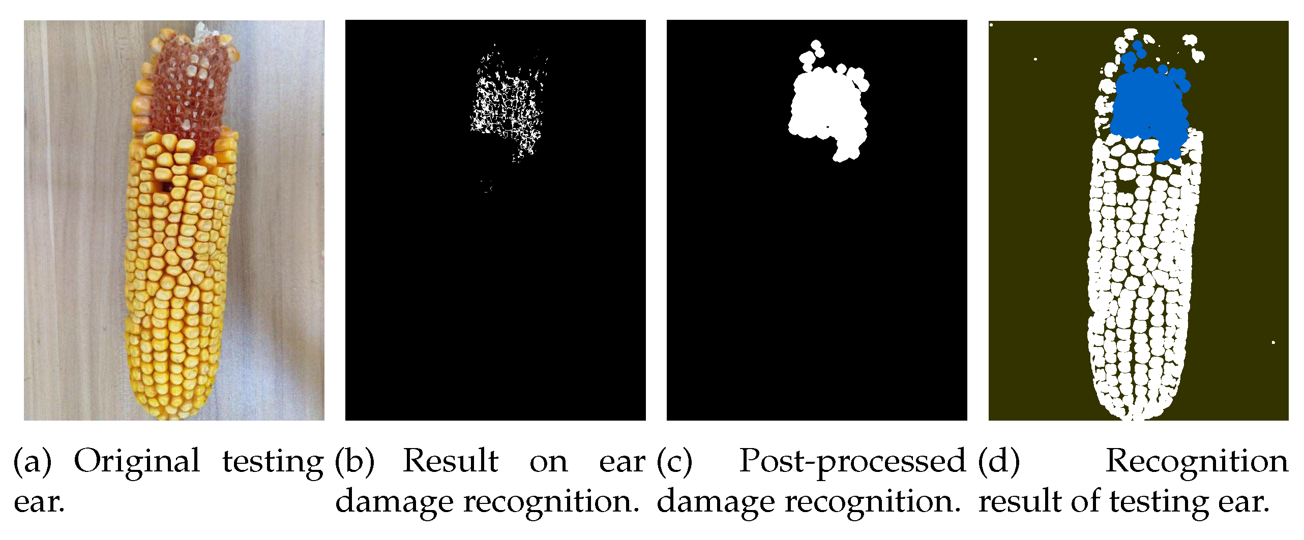
In previous operations, we obtain the region of corn kernels. Next, we introduce the method to recognize ear damage. The strategy is mainly based on the distinguishing reflections of kernel-dropping region in the red, green, and blue bands. We set the thresholds for upper and lower bounds of the three bands, respectively. A pixel is regarded to belong to ear damage region only when its reflections of all three bands are in the range of thresholds. The detailed steps are provided in Algorithm 5. The input matrix ${\mathit{C}}_3$ is just the image obtained after kernel recognizing, corroding, and expanding operations (see Figure 6c). All white pixels of ${\mathit{C}}_3$ are regarded as kernels, such that they will not be considered in the process of ear damage recognizing. The results is presented in Figure 7b. We can note the recognized pixels are consistent with the actual damaged region. However, they are dispersed and cannot form a complete region. This is because many stubbles exist along the kernel-dropping region. These stubbles do not have the same RGB features as kernel-dropping region, and, therefore, they cannot be recognized directly by Algorithm 5.

Algorithm 5 Recognizing ear damage.

Require: Original objective RGB image $\mathit{X}\in {\mathcal{R}}^{n_1\times n_2\times 3}$, binary image ${\mathit{C}}_3\in {\mathcal{R}}^{n_1\times n_2}$.  1: Initialize ${\mathit{C}}_4=\mathit{0}\in {\mathcal{R}}^{n_1\times n_2}$;  2: for each pixel ${\mathit{C}}_3(i,j)$ do  3: if $\delta \left({\mathit{C}}_3(i,j)\right)=0$ then  4:  Let $x^r=\mathit{X}(i,j,1)$, $x^g=\mathit{X}(i,j,2)$, and $x^b=\mathit{X}(i,j,3)$;  5:  if $80<x^r<160$, $30<x^g<70$, and $30<x^b<70$ then  6:   ${\mathit{C}}_4(i,j)=1$;  7:  end if  8: end if  9: end for Ensure: Outputted binary image ${\mathit{C}}_4$.

To address this problem, we propose the post-processing strategy that is summarized in Algorithm 6. The corrosion step and the expansion step are alternatively executed until the termination condition is reached. Here, the termination condition is also composed of two judgements. The first is whether the number of iterative cycles is enough. The second is whether the outputted image is the same as the inputted image in an iterative cycle. The proposed strategy can be regarded as a kind of close operation, aiming to connect spreading pixels in damage region and eliminate isolated pixels that are misidentified. We utilize Algorithm 6 for Figure 7b with $\lambda =3$ and $\rho =4$. The post-processed image is presented as Figure 7c. Obviously, the complete region is obtained instead of spreading pixels. The region is consistent with the damage region of the testing ear. As shown in Figure 7d, we combine the results on corn kernel recognition and ear damage recognition to obtain the final recognition result, where the black, white, and blue regions represent the background, the corn kernels, and the ear damage, respectively. The outline of complete method is summarized in Figure 8.

Algorithm 6 Post-processing of ear damage recognizing.

Require: Binary image obtained through ear damage recognizing ${\mathit{C}}_4\in {\mathcal{R}}^{n_1\times n_2}$, maximum number of iterative cycles $t_{max}$.  Initialize $\mathit{H}={\mathit{C}}_4$;  while termination condition is not reached do   Corrode $\mathit{H}$ to obtain $\mathit{J}$ using Algorithm 3 with 1 iterative cycle;   Expand $\mathit{J}$ to obtain $\mathit{H}$ using Algorithm 4 with 1 iterative cycle;  end while  Set ${\mathit{C}}_5=\mathit{J}$; Ensure: Outputted binary image ${\mathit{C}}_5$.

3. Experimental Results and Discussion

The experiments were composed of two parts, the experiments on single ear recognition and those on multiple ears recognition. The test images used for multiple ear recognition were acquired in the ear collection box during harvesting. All experiments were performed using Matlab 2014 software.

3.1. Results on a Single Ear

Three damaged ears were employed for this part of experiments. The original values of pixels with respect to each band were 8 bit so that the range of values is 0–255. The parameters $\beta$ and ${\gamma }^r$ for Algorithm 2 were set to ${10}^3$ and 170, respectively. For the corroding process, the parameter $\lambda$ was set to 3 and the maximum number of iterative cycles was set to 5. For the expanding process, the parameter $\rho$ was set to 4 and the maximum number of iterative cycles was set to 1.

The results given in Figure 9, Figure 10 and Figure 11 present the kernel recognition results, the damage region recognition results, and the final results, respectively. Figure 9 shows that the contours of ears are drawn precisely for all ears. The kernels are recognized accurately except a small number of broken kernels. In Figure 10, we can see the results on damage recognitions and their post-processing images. Even though the recognized pixels of damage region are dispersed, they are extended to be whole regions by the post-processing algorithm. As there is no impurity contamination in the experiments on a single ear, few outliers of damage region recognitions appear before post-processing. Combining the kernel recognitions and damage region recognition, the final recognition results are provided in Figure 11. By comparing the original images and the final results, we can note their structures are highly consistent with the actual damage regions, indicating the practicality and accuracy of the proposed method.

3.2. Results on Multiple Ears

Next, we conducted experiments on multiple ears, i.e., the actual scenes of peeled corn ears during harvesting. Five test images were employed for this part of experiments with the spatial size of $600\times 800$. These test images contained all common objects in corn ear harvesting, including complete ears, damaged ears, impurities, and backgrounds. The parameter settings were the same as those used in the experiments on a single ear. Similar to the results on a single ear, we also provided the results on multiple ears of three procedures that are shown in Figure 12, Figure 13 and Figure 14, respectively. In Figure 12, we can see that, although the shooting angle, illumination, and definition for five scenes are somewhat different, the contours and kernels are recognized successfully. The outliers of kernel recognition are obviously eliminated via the corroding operation, especially for Scenes 4 and 5. Figure 13 shows the cooperative use of the damage recognition algorithm and the post-processing algorithm realize the determination of damage regions of all corn ears in the scenes.The results are presented in Figure 14 where three types of regions are marked. The first is the damaged regions that are successfully recognized. The second is the damaged regions that are not recognized, i.e., missed damaged regions. The third is the recognized regions that are not the actual damaged regions, i.e., false recognized regions. The metric recognition rate was employed to evaluate the performance of the proposed method, which is defined as the ratio between the number of successfully recognized regions and the number of all damaged regions. The recognition rates for each scene are summarized in

Table 1. Summary on recognition rates for test scenes.

	Number of All Damaged Regions	Number of Recognized Regions	Recognition Rate (%)
Scene 1	6	6	100.00
Scene 2	10	8	80.00
Scene 3	9	9	100.00
Scene 4	11	11	100.00
Scene 5	7	7	100.00
Total	43	41	95.35

. Only two damaged regions in Scene 2 are missed, and the overall recognition rate is 95.35%, demonstrating that most damaged regions can be successfully recognized by using the proposed method. On the other hand, a few false recognitions can be noted in the results. The reason is the RGB data of some pixels in the wrong regions satisfy the constraint given by Step 5 of Algorithm 5. These pixels are located as a whole region and are not completely eliminated by the corroding operation. Therefore, they are recognized by the damaged region by mistake. Fortunately, the falsely recognized regions are extremely small and can be ignored.

4. Discussion

Based on the experimental results, several issues are discussed as follows.

• In this study, we subjectively evaluated the recognition performance. For an objective image, especially for a multiple ear image, the recognition accuracy was determined by several aspects, such as the position of damage region, the area of damage region, and the contour accuracy of ears. Hence, one or more indicators may be required to objectively evaluate recognition performance. This is of great valuable for further study.
• As shown in Figure 12, wrapped leaves are recognized as kernels. This is because the RGB data of leaves are also added into the training samples in the dictionary learning process. The ears wrapped by leaves imply they are not peeled thoroughly. Such ears are usually complete without damage, and, therefore, in this study, we treated the wrapped leaves as kernels.
• We utilize the dictionary learning method to recognize kernels, while using thresholding method in terms of RGB reflections to recognize damage. This is because the characteristic of RGB reflections for ear damage is distinctive, and it can be easily distinguished through RGB reflections. However, as mentioned above, the RGB reflections of corn kernels are close to some impurities. Additionally, the RGB reflections of kernels for different corn varieties are also different. Hence, we trained dictionaries in advance to recognize kernels based on the correlation between dictionaries and objective images.
• In the experimental results on multiple ears, only two damaged regions are missed among all test scenes. As shown in Figure 14, one missed region (Figure 14, left) is located near a cracked ear. The cross-section faces right to the camera, and therefore the damaged circumferential surface is not imaged, leading to the failure of recognition. The other missed region (Figure 14, right) shows atypical RGB data on its damaged surface such that they do not satisfy the constraint of the recognition algorithm.
• In this study, we theoretically developed the method of peeling damage recognition. We believe the proposed method can be applied for practical harvesting in the field. The realization should rely on a RGB camera and an embedded control system that are fixed into the harvesters. The images acquired by the RGB camera are transmitted to the embedded control system where the recognized process is executed based on the proposed method.

5. Conclusions

We propose a method for corn ear damage recognition, including the recognition of corn kernels and that of ear damage regions. For this purpose, we introduce the algorithms for each process, including dictionary learning, corn kernel recognition, image corrosion, image expansion, ear damage region recognition, and post-processing. We also present the experiments using test images for both single ear and multiple ears. Experimental results demonstrate the practicality and accuracy of the proposed method.

There are still some issues that require further study. More experiments in terms of different corn varieties need to be conducted to verify the performance of the proposed method. The embedded control system, including the hardware and software, should be developed for practical experiments in the field. Additionally, as mentioned in Section 4, the accurate recognition of the damaged regions that exhibit the atypical RGB data requires further study.