1. Introduction
Formation tracking control of multiple underactuated surface vessels (USVs) has aroused great interest in recent years, owing to the fact that a team of USVs working together can accomplish more challenging missions than a single USV, such as surveillance, autonomous exploration, reconnaissance and perimeter security. A significant amount of research efforts has been focused on the control of multiple USVs. There are some challenges in USVs formation control, which are still worth mentioning. The first challenge is the amount of information being exchanged among the USVs in formation tracking control. In the beginning, USVs could sense their own positions, which are presented in a global coordinate system. Every USV controls its own positions to achieve the desired formation, which is prescribed by the desired positions in the global coordinate system [
1,
2,
3]. The desired trajectory is available for all USVs. In this case, interactions are not necessarily needed because the desired formation can be achieved by position control of individual USVs [
4]. This means that every USV should be equipped with advanced sensors, but this may not be practical. Considering the limitation of sensors, a distributed control law was proposed based on graph theory in [
5,
6,
7,
8]; it requires interactions to extract information from neighbors. The leader-following consensus problem of networked Lagrangian systems was investigated in [
9]; both unknown control directions and uncertain dynamics were taken into consideration. Two types of distributed control protocols were proposed base on undirected graphs and directed graphs.
Output constraint is a challenge to USVs. A coordination strategy for multi-agent formation control based on a constraint function was proposed in [
10]; this method could stabilize the formation error under a bounded tracking error assumption. A cooperative controller for a group of
N USVs with limited sensing ranges was proposed in [
11]; a novel potential function was used to solve the collision avoidance problem. Output-feedback cooperative controllers for mobile robots were designed in [
12], where limited sensing was considered, and a control system based on potential functions incorporated with jump functions was designed. In [
13], a group of USVs with a leader was considered, in order to make sure USVs function under asymmetric range and bearing constraints, the control design incorporated an asymmetric barrier Lyapunov function (BLF), and a fast convergent observer was designed to estimate the velocity of the leader. A nonlinearly transformed formation error without considering input saturation was developed in [
14]; collision-avoiding, connectivity-preserving and limited communication ranges were considered simultaneously, and a distributed controller using the transformed error was designed for each USV.
In practice, designing a controller without considering the input saturation factor may lead closed-loop systems to instability. In [
15], a basic controller base on two feedback functions was proposed, and the functions ensure the realization of the expected formation and input constraint. In [
16], an output feedback controller was proposed by using additional controllers that are able to deal with the input saturation and underactuated problems simultaneously. In [
17], an adaptive steering control method for uncertain ship dynamics with input constraint was designed; the method ensures the performance of the system under changing environmental conditions. In [
18], uncertain strict-feedback nonlinear systems with input saturation and unknown disturbances were investigated, a dynamic surface control (DSC) combined with a backstepping method was proposed, and the effect of input saturation was approximated using a radial basis function neural network (RBFNN).
The model uncertainties and environmental disturbances are an important challenge. To overcome these difficulties, a hub motion estimation algorithm was designed in [
19], where sensor fusion was employed. A controller that forces a USV to track arbitrary reference trajectories was proposed in [
20]; a disturbance observer was presented to estimate environmental disturbances. In [
21], an adaptive fuzzy controller for USV exposed to ocean currents and time-varying sideslip angle was designed, the dynamic uncertainties and environmental disturbances could be compensated by the fuzzy logic system. A practical adaptive sliding mode controller for an USV was proposed in [
22], where an RBFNN combined with minimum the learning parameter method was designed to approximate the uncertain system dynamics online. In [
23], neural network (NN)-based tracking control of underactuated systems was surveyed; unknown parameters and matched and mismatched disturbances were considered, and an adaptive control scheme incorporating multi-layer NNs was proposed.
In most of the above papers, the controller is designed by using the backstepping method, and Lyapunov function is used to analyze the stability of the system. In backstepping design, the computer explosion problem is universal. Tracking differentiators were used to solve the problem in [
14].
Inspired by the above, in this paper we simultaneously consider model uncertainties, environmental disturbances, input saturation, collision avoidance and the limitations of communication distance. An extended state observer (ESO) is used for observing model uncertainties and environmental disturbances. A nonlinearly error transformation is provided for achieving the connectivity preservation, the collision avoidance and the distributed formation tracking. The USVs are interconnected through a directed communication network. Auxiliary variables are introduced to solve input saturation and the underactuated problem. Tracking differentiators are employed to calculating derivatives of virtual control variables. Finally, a distributed control law for each USV is constructed. The stability of the total closed-loop system is analyzed via Lyapunov theory.
The main contributions of this paper are summarized as follows. First, compared with [
13], unknown model dynamics and environmental disturbances are estimated by ESO, and graph theory is combined with a distributed controller, which makes the controller suitable to be readily applied to formation control. Second, compared with [
14], BLF is introduced into nonlinearly transformed formation error. In order to cope with input saturation, auxiliary variables are introduced into controller design.
The rest of this paper is organized as follows. The models of USVs, ESO and graph theory are introduced and the USV formation control problem is formulated in
Section 2.
Section 3 proposes a distributed controller and presents the stability analysis. Simulation results are shown and discussed in
Section 4.
Section 5 summarizes.
2. Preliminaries and Problem Formulation
2.1. Notion
The following notations will be used throughout this paper. is the absolute value. (.) and (.) represent minimum and maximum eigenvalue of a square matrix, respectively. represents the Euclidean norm. is diagonal matrix. represents the dimensional Euclidean Space. represents the dimensional identity matrix. i is used as the index of the USVs, i.e., .
2.2. Graph Theory
Graph theory is used to describe the communication topology of USVs. A directed graph consists of a vertex set and . describes that information of the jth USV is available to the ith USV. The ith USV and the jth USV are said to be neighbors if , where , and is the distance between the ith USV and the jth USV. The neighbors of the ith USV are described by .
Assumption 1. The total graph G is directed at and G has a directed spanning tree with the root node being the leader node.
2.3. Model of USVs
A group of USVs consisting of a leader and
n followers are considered. Assume that the
ith USV has an
-plane of symmetry. Heave, pitch and roll motions are neglected. The body-fixed frame coordinate origin is set in the center-line of the USV. The mathematical model of the
ith USV is defined as [
24]:
where
is the vector denoting the ship position
and yaw angle
with coordinates in the earth-fixed frame, and
is the vector denoting surge, sway and yaw velocities of the
ith USV in the body-fixed frame.
is the vector representing environmental disturbances.
is the control vector of the
ith USV, which consists of the surge force
and yaw moment
. The matrices
are given by
is the inertia matrix of the
ith USV. Here, we assume that the inertia matrices are diagonal.
represents a skew-symmetric matrix of Coriolis and centripetal term.
is a nonlinear damping matrix.
The model of leader is defined as follows: a subscript “0” denotes the leader whose position
is generated by
Assumption 2. , , , are bounded, and the data are available only for the ith USV satisfying .
Assumption 3. The disturbances , , are unknown but bounded so that , is a unknown positive constant.
Assumption 4. and are assumed unknown.
2.4. Input Saturation
Considering input saturation, control vector
is defined as follows:
where
and
are the maximum and minimum control force and moment, respectively.
Define the mismatch function between input without saturation and with saturation as
, where
with
and
are surge force and yaw moment calculated by the distributed controller, respectively. The saturated control in (
1) is given by
.
2.5. Extended State Observer
In this section, an ESO is used for estimating total disturbances consisting of the unknown term of the system matrix
,
and environmental disturbances
[
25]. The
ith USV dynamic (
1) is rewritten as
where
is total disturbances; it is a state vector expressed as
.
The following assumption is made during ESO design.
Assumption 5. There exists a positive constant satisfying .
Remark 1. Note that . The velocity is bounded, and control inputs to drive USVs are bounded, and thus the derivative of is bounded. According to Assumption 3 and the disturbances are bounded, the derivative of is bounded. Then, Assumption 5 is reasonable.
An ESO is used for estimating the total disturbances as follows:
where
,
,
,
,
,
,
,
,
,
,
,
are the estimates of
,
,
,
,
,
,
,
and
.
,
and
are gain matrices.
From (
5) and (
6), the error dynamics of the observer can be expressed as
where
,
and
are estimation errors. (
7) can be rewritten as
where
,
and
Theorem 1. Consider the system (5) under Assumptions 2–5, the proposed observer (6) guarantees estimation error is bounded. Proof. Consider the following Lyapunov function candidate as
differentiating
with respect to time and using (
8),
using Young’s inequality and Assumption 5,
, then
Select the appropriate parameters
,
and
to make sure
. Equation (
12) shows that the observer (
6) ensures that the estimation error is bounded. □
2.6. Barrier Lyapunov Function
Definition 1 ([
26]).
BLF is a scalar function, defined with respect to a system on D, which is continuous, positive definite, and an open region containing the origin. BLF has continuous first-order partial derivatives at every point of D and the property as x approaches the boundary of D, and satisfies , along the solution of for and some positive constant b. To deal with the output constraint, a BLF is introduced as
where
is a constant and
z is variable of error.
Lemma 1. If , is any constant [26], then 2.7. Problem Formulation
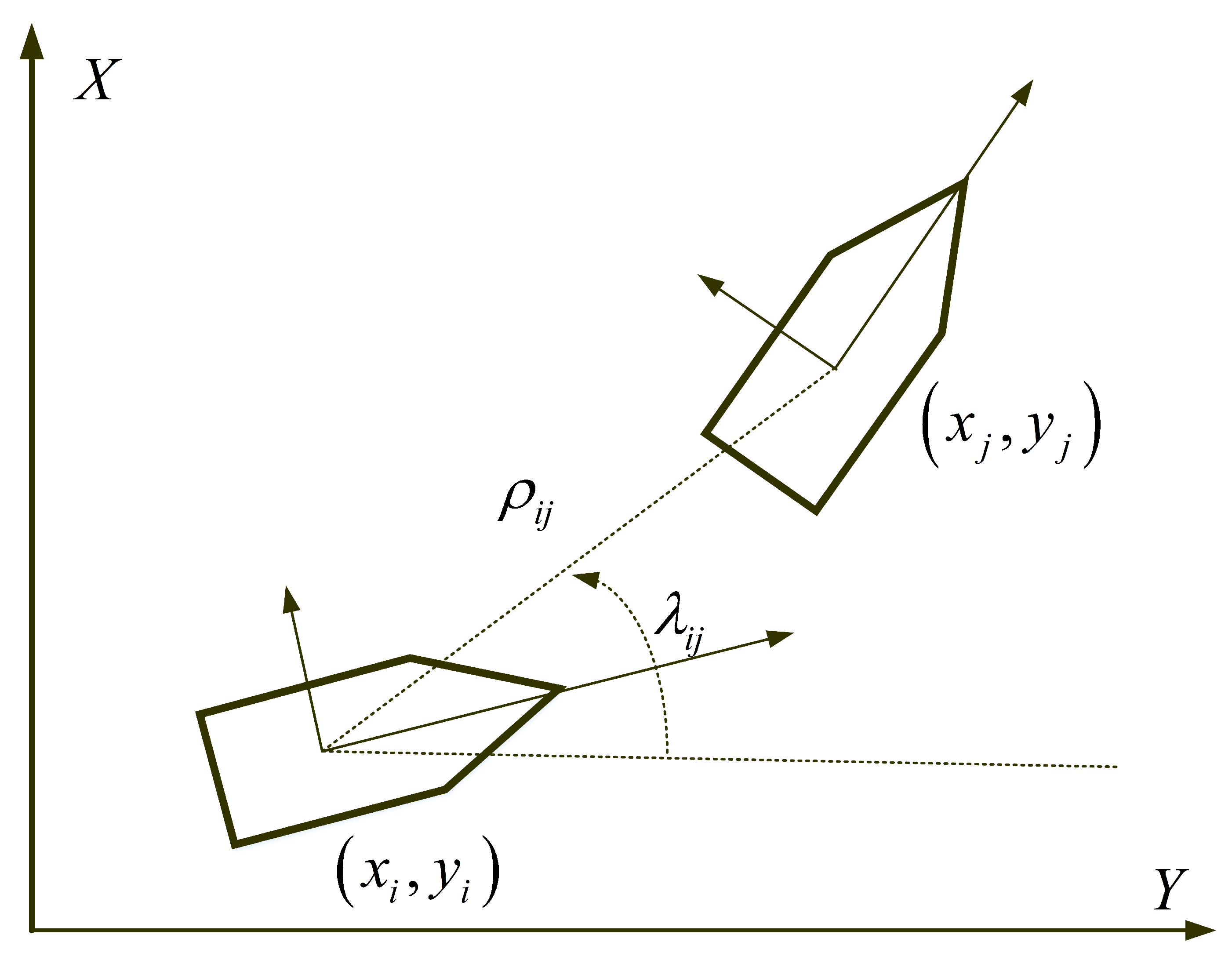
As shown in
Figure 1,
is defined as the relative distance between the
ith USV and the
jth USV; its equation and differential equation are given as follows:
is defined as the relative angle between the
ith USV and the
jth USV; its equation and differential equation are given below:
The relative information and can be measured by using local sensors, such as lidar and the gimbaled camera. If the ith USV and the jth USV are said to be neighbors, the ith USV is able to obtain the data and directly.
The control objective is to design a distributed controller for the ith USV to track the leader with model uncertainties, input saturation and limited communication ranges. Specifically, it is to achieve the following two objectives.
- (1)
and .
where , and are minimum avoidance ranges of the ith USV and the jth USV, respectively. , and are maximum communication ranges of the ith USV and the jth USV, respectively. and are the minimum and maximum bearing angle of the ith USV.
- (2)
and .
where and are positive constants that can be made small enough.
Remark 2. Objective (1) means that the connectivity preservation and the collision avoidance are considered if the ith USV is a neighbor of the jth USV. Objective (2) represents the formation tracking problem.
3. Controller Design
In this section, the distributed controller is designed to meet the requirements of connectivity-preserving and collision avoidance. To satisfy these requirements, nonlinearly transformed error surfaces are introduced as follows:
where
if the
ith USV and the
jth USV are neighbors, otherwise
.
and
will be explained later.
is the approach angles expressed as:
where
is a positive constant,
,
is virtual control and
,
is the signal derived from the following first-order low-pass filters
, and
is constant.
,
is a time-varying and bounded auxiliary variable derived to deal with the underactuated problem and input saturation.
Inspired by the proposed asymmetric BLF method in [
26], a nonlinearly transformed formation error combined with modified BLF was developed to achieve the connectivity preservation and the collision avoidance. Error surfaces
and
are defined as follows:
where
,
,
,
,
and
.
Remark 3. The error surfaces and are introduced to realize the connectivity preservation and the collision avoidance. According to definition of objective (1) , then . From definition of and , such that . One notes that and , thus if and if . It holds that the connectivity preservation and the collision avoidance are achieved as if and if . From Equation (32), the definition of implies . According to the definition of , if , if . Then the distance constraint can be satisfied. The angle constraint is similar to the distance constraint. A distributed controller using the nonlinearly transformed error is presented.
- Step 1:
Differentiating
along (
17) and (19) yields
where
,
,
and
. Then,
is rewritten as follows:
where
and
In these expressions, are the elements of the set .
Define , and is bounded and , is an unknown positive constant.
Remark 4. From the definition of , and and Equations (41)–(43), one notes that , and are bounded, so is reasonable. In order to stabilize
, the desired virtual control
is given as:
where
,
,
is a positive definite matrix,
are the elements of the set
,
,
, and
is a constant. Notice that the matrix
is invertible owing to
. Notice that based on Lemma 1, we have
and define
, then
.
- Step 2:
Differentiating
along (
21) yields
where
and
.
The stabilizing function
is chosen as:
where
is a positive constant.
Remark 5. The virtual controllers (46) and (49) are composed of the error surfaces (20) and (21), the distributed vectors , and matrices and . The link weights of the distributed error surfaces (20) and (21) depict the directed graph among USVs that satisfies Assumption 1. Thus, the proposed formation approach is in a fully distributed formation manner. - Step 3:
Differentiating (
22)–(
24)
The update law of additional controls
,
and
is given by
where
,
and
are positive constants.
- Step 4:
To stabilize the system, kinetic control laws are designed as
where
and
are positive constants.
Theorem 2. Consider that the system consist of USV (1), the control law (56) and (57), the observer (6) and the update law of additional controls (53)–(55), with environmental disturbances, input saturation and limited communication ranges under Assumptions 1–5. The proposed controller guarantees all signals in the closed-loop system are bounded and two objectives are achieved. Proof. Consider the Lyapunov function as follows:
along with (
40), (
48) and (
50)–(
52), the differentiation of
V is given as
where
.
Furthermore, substituting virtual controls (
46) and (
49), additional controls (
53)–(
55), control laws (
56) and (
57) into (
59) leads to
where
,
,
,
and
.
From the definition of
and
, the following can be attained.
where
. From [
27], we have
According to
and
, we have
According to Young’s inequality, then:
Equation (
60) can be rewritten as follows:
where
.
Define
, then
Consider the total function
Using (
12), (
68) and (
69), the derivative of
is given by
where
,
and
. According to Young’s inequality,
with
being a small positive constant and
. Consider the sets
and
where
and
are positive constants. Since
is compact in
, there exist a constant
such that
on
.
Choosing
with
, and constants
and
with
is a constants. The following can be attained:
Owing to
on
, the inequality (
72) becomes
where
. This implies that:
From the definition of , it can be concluded that is bounded. From Assumption 1, there exists i and j such that for where and . From the definition of , the boundedness of leads to and . Thus, if for , then and . This completes the proof of (1).
From (
74),
exponentially converges to the compact set
that can be made arbitrarily small by adjusting
. From (
20),
and
can be reduced to be arbitrarily small; this leads to the conclusion that
and
can be also reduced to be arbitrarily small. Then, it holds that
and
, and the proof of (2) is completed. □
The distributed controller is composed of the local virtual control laws (
46) and (
49) and the auxiliary dynamics and the actual control laws (
56) and (
57). In (
1), there is no control input on the sway dynamics, and this causes difficulty in the control of sway. To make sure of the stability of the sway dynamics, auxiliary variable
is introduced to solve the problem, and auxiliary variables
and
are introduced to solve the problem of input saturation. The
function guarantees that the introduced variables
,
are smooth and differentiable. By designing
in (54) and substituting it into (
59), the boundedness and convergence of
can be achieved.
According to (
72), the following conditions determine the stability of the entire system:
,
,
,
,
, and
. According to (
13), the size of the eigenvalues of parameters
,
and
determines the convergence speed of estimation error. Note that
affects both the stability of the observer and of the whole system.
4. Simulation Results and Discussion
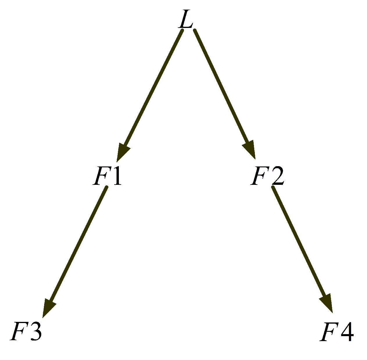
In this section, the formation is composed of one leader and four followers. From the defined heterogeneous communication and avoidance ranges, the directed communication graph is given in
Figure 2. The model of USV is taken from [
28], and the main parameters are
,
Environmental disturbances are chosen as a superposition of zero mean white noise and constant interference. Standard deviation of white noise is chosen as 0.4, constant interference is chosen as 0.1. The parameters for ESO are set to
,
, and
. The control forces and moment are constrained as
,
,
, and
. The design parameters of control laws are chosen as
,
,
,
,
,
, and
. The heterogeneous communication ranges of USVs are
m,
m,
m,
m and
m. The avoidance ranges are
m and
. The path of the leader is generated by
m/s and
rad/s for
s,
m/s and
rad/s for
s,
m/s and
rad/s for
s. The initial positions of USVs are chosen as
m, 0 m, 0 rad
,
m,
m, 0 rad
,
m, 5 m, 0 rad
,
m, 8 m, 0 rad
,
m,
m, 0 rad
. Desired distances and angles are chosen as
m,
rad,
rad,
rad, and
rad.
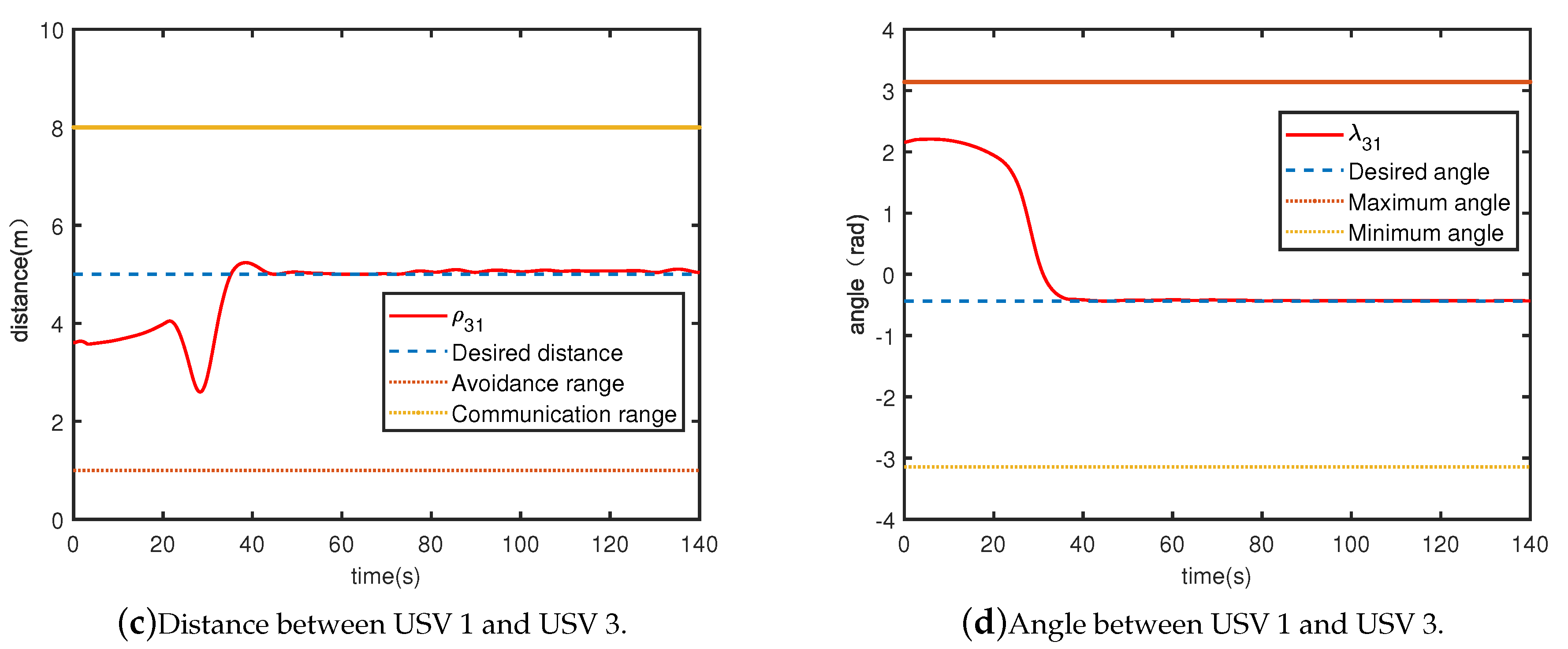
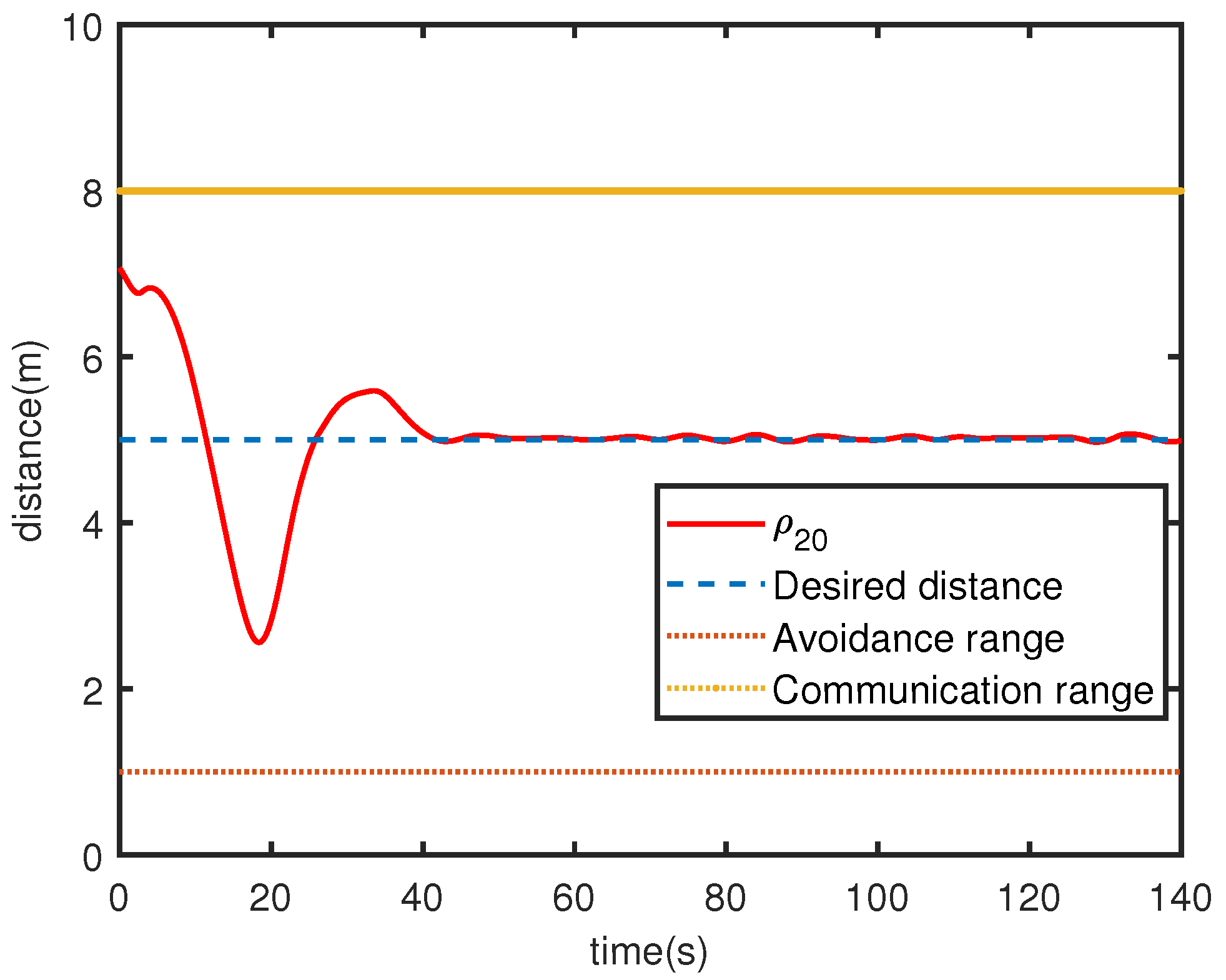
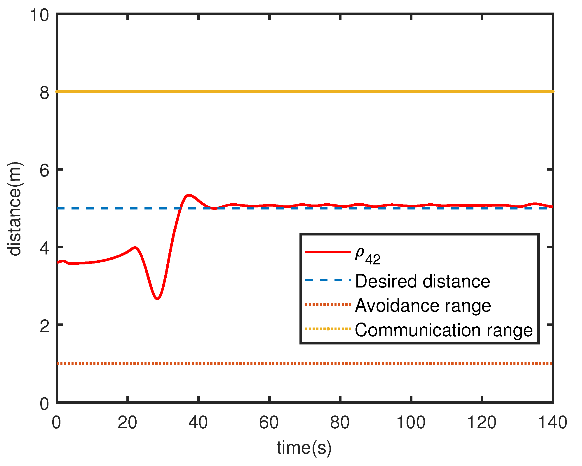
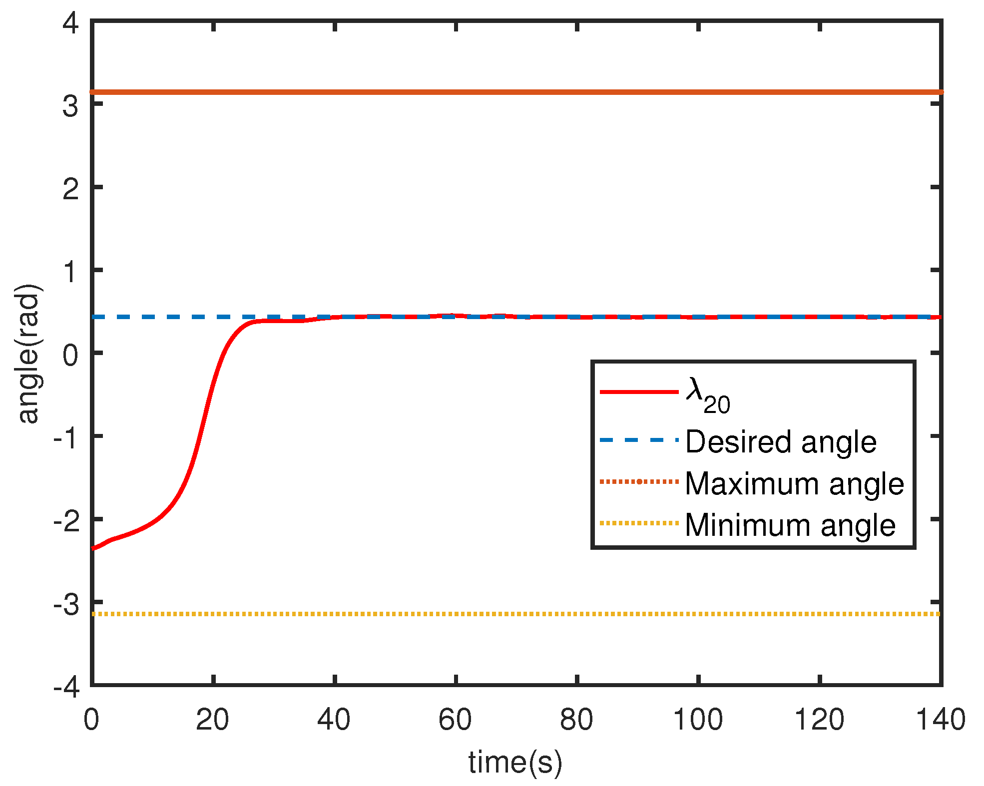
The formation tracking result is shown in
Figure 3.
Figure 4a,c,
Figure 5 and
Figure 6 show the the distance errors
, and
Figure 4b,d,
Figure 7 and
Figure 8 show the angle errors
. As shown in
Figure 3, one can see that all the USVs are able to track the formation.
Figure 4,
Figure 5,
Figure 6,
Figure 7 and
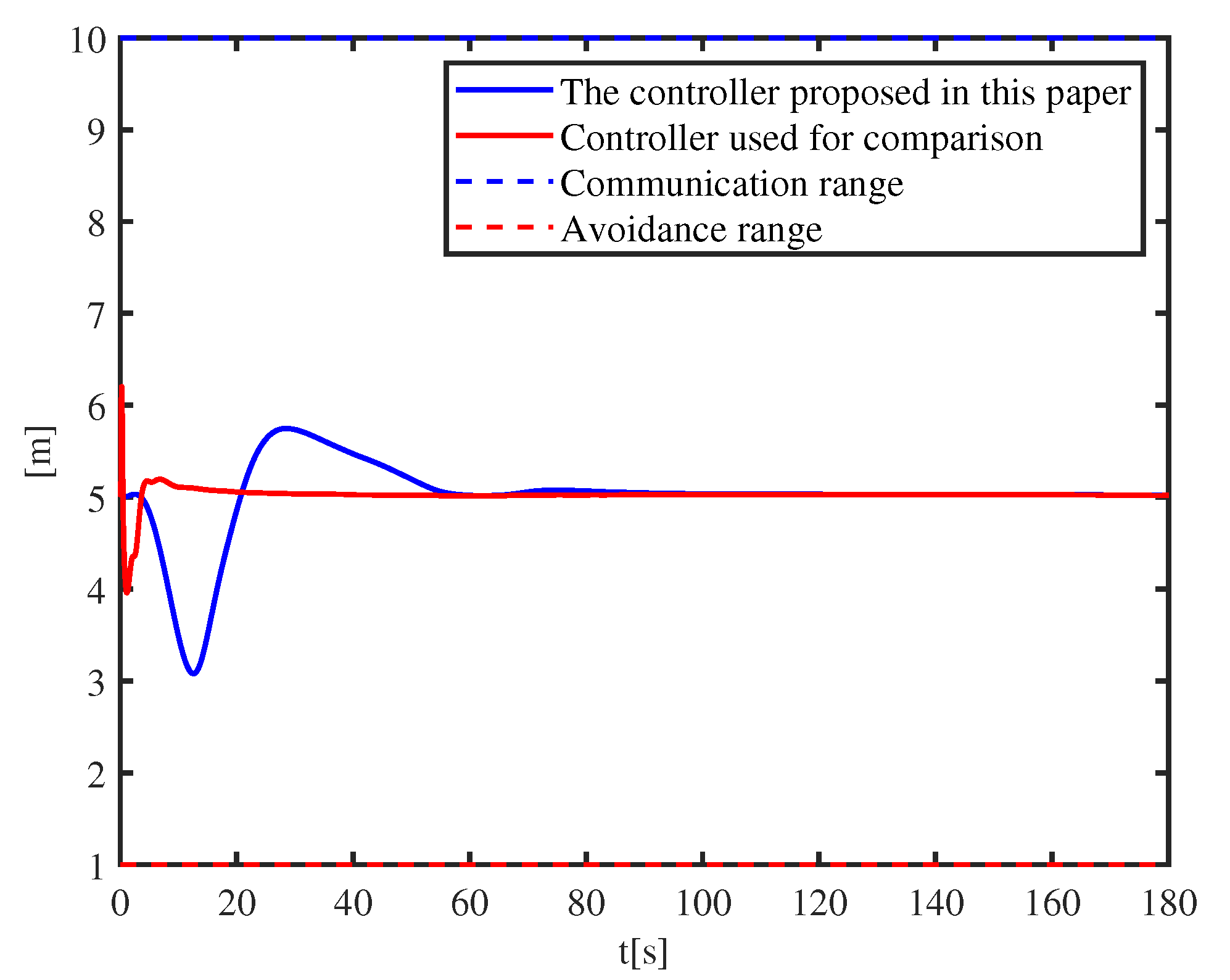
Figure 8 show trends of relative distance and angle, and the connectivity-preserving and collision-avoiding is achieved.
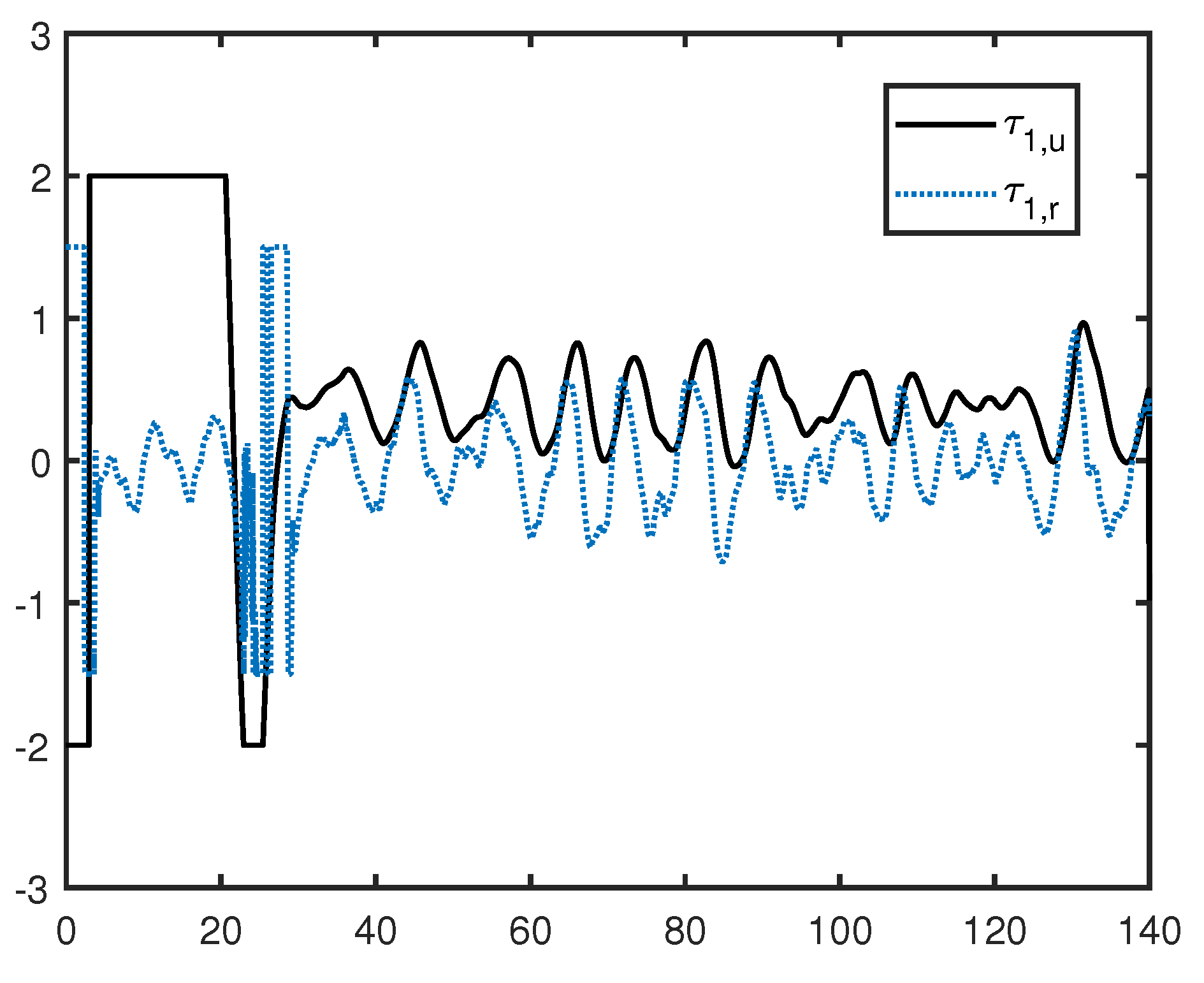
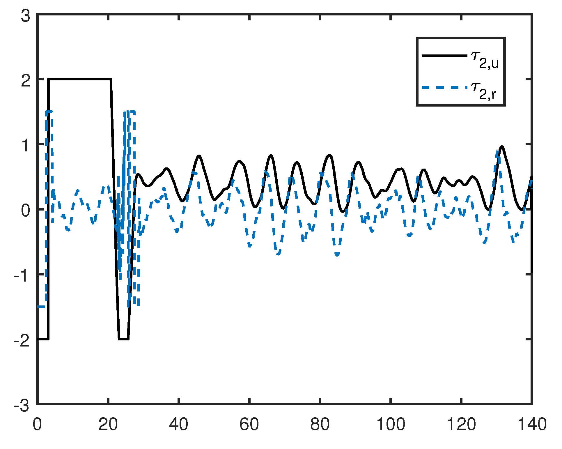
Figure 9,
Figure 10,
Figure 11 and
Figure 12 depict the control inputs of the follower. In the beginning, since the initial heading angles of followers are 0 rad, all followers turn around and travel in the opposite direction for a certain period of time, then the followers take a turn to avoid collision, and the control inputs
are saturated and suffer from sudden jumps. The control inputs
become smaller and unsaturated when the follower catches up with the leader.
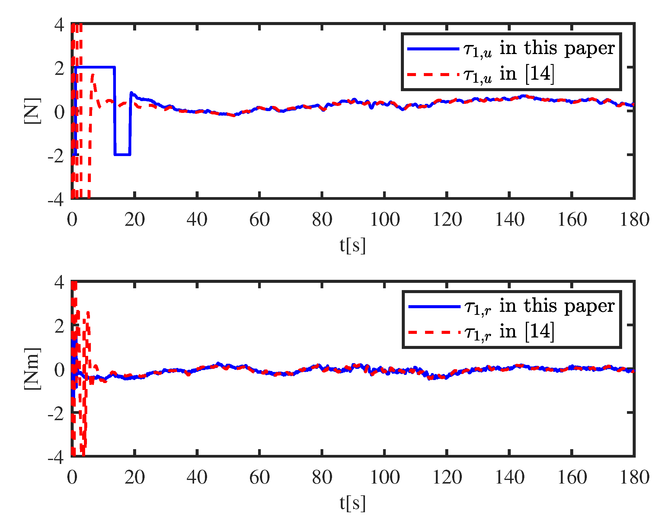
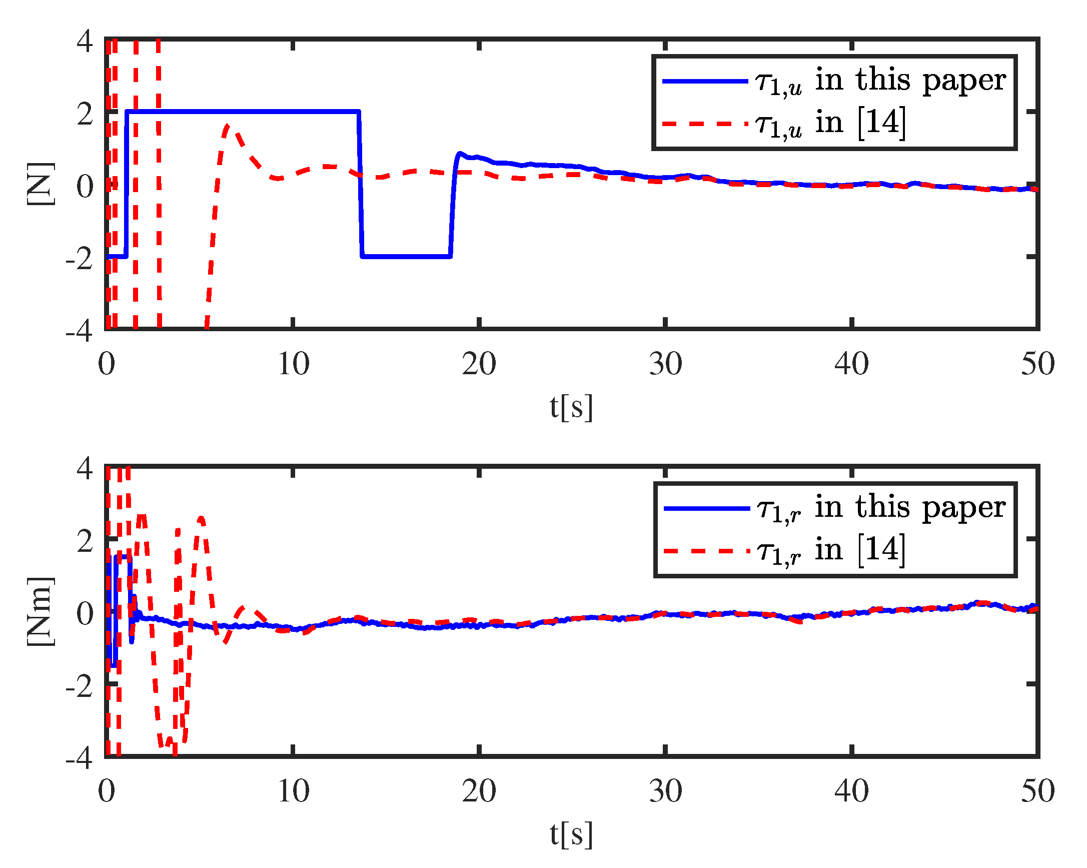
Comparison with the controller proposed in [
14] is given though Matlab simulation in
Figure 13,
Figure 14,
Figure 15 and
Figure 16; the simulation result is provided to validate the effectiveness and feasibility of the proposed controller. Comparison is designed under the same environmental disturbances, and the standard deviation of white noise is chosen as 0.4 while the constant interference is chosen as 0.1, with the same initial position
m,
m, 0 rad
and the same objective
and
rad.
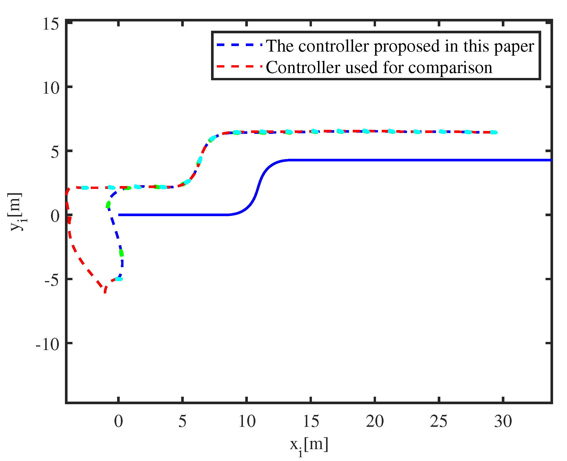
Figure 13 shows that USV 1 could track the leader accurately in a different controller.
Figure 14 shows that the controller proposed in [
14] accomplishes faster convergence and tracing speed. Not taking input saturation into consideration, the result is a more aggressive tracking trajectory, which is difficult to implement. In
Figure 15, control inputs under different controllers are given. A local enlarged drawing of the control input is given in
Figure 16. In the beginning, the input signal in this paper is saturated, and the position of the USV changes relatively slowly. At about 60 s, the follower catches up with the leader. The input signal in [
14] is huge, and the position of the USV changes rapidly. At about 10 s, the follower has caught up with the leader. Unlike the controller proposed in this paper, it is extremely difficult to avoid a huge input signal and a drastic change of input signal.
By using the modified barrier Lyapunov function, the connectivity preservation and the collision avoidance are achieved. By using ESO and the proposed controller, the followers can track the leader accurately. By using an auxiliary variable, the input saturation is solved. Positive definitions of matrix , and make sure that convergence of estimation error is achieved. By adjusting , the track error can be made arbitrarily small.
Both controllers are designed based on Assumption 2, and
,
,
,
are bounded, meaning that the formation control problem is solved only when the follower starts in a certain neighborhood of the leader. In [
29], the path following the control problem of USVs was investigated and the system could provide global asymptotic stability. How to design a controller which could makes the system have global asymptotic stability is an interesting challenge. Both controllers are designed without considering the saturation rate of the actuator, meaning that the conclusion is relatively radical. How to design a controller with the rate saturation factor for formation control will be considered in future work.

