How Deeply to Fine-Tune a Convolutional Neural Network: A Case Study Using a Histopathology Dataset

Abstract

Accurate classification of medical images is of great importance for correct disease diagnosis. The automation of medical image classification is of great necessity because it can provide a second opinion or even a better classification in case of a shortage of experienced medical staff. Convolutional neural networks (CNN) were introduced to improve the image classification domain by eliminating the need to manually select which features to use to classify images. Training CNN from scratch requires very large annotated datasets that are scarce in the medical field. Transfer learning of CNN weights from another large non-medical dataset can help overcome the problem of medical image scarcity. Transfer learning consists of fine-tuning CNN layers to suit the new dataset. The main questions when using transfer learning are how deeply to fine-tune the network and what difference in generalization that will make. In this paper, all of the experiments were done on two histopathology datasets using three state-of-the-art architectures to systematically study the effect of block-wise fine-tuning of CNN. Results show that fine-tuning the entire network is not always the best option; especially for shallow networks, alternatively fine-tuning the top blocks can save both time and computational power and produce more robust classifiers.

1. Introduction

Medical images play a very crucial role in patient treatment; however, usually, the shortage of manpower, the time required to reach a decision, and the need for a second opinion are factors that greatly impact the process. Correctly and more quickly classifying images is an absolute need for certain medical images fields, like pathology. Histopathology images are very important for detecting certain kinds of diseases like cancer or even determining the kind of cancer itself to see if it is benign or malignant and its degree. Histopathology is defined as examining a tissue sample taken by a biopsy to diagnose certain diseases microscopically [1]. It plays a very important role in the detection of diseases, enabling doctors to carefully create a treatment plan. The physician who is responsible for classifying histopathology images is called a pathologist. The image-examining process is extremely difficult and requires an experienced pathologist with years of experience. In the United States, the number of active pathologists dropped 17.5% in the last decade while the workload increased by 41% [2], which indicates a real need for assisting the pathologists in their work by providing them with an autonomous classifier that is able to classify histopathology images with a high level of accuracy.

A recent breakthrough in the artificial intelligence field is machine learning, in which an algorithm can be developed that will be able to extract image features automatically. When the algorithm used is a neural network with more than one hidden layer, it is called deep learning. Deep learning can be implemented in the image classification domain in which a feed-forward convolutional neural network (CNN) [3] can be used to classify images automatically. Making the CNN able to classify images is called training; in training, the CNN’s weights will be adjusted to suit the image dataset under study. The main point of CNN is that it is able to map important features of images that can be used to classify those images without the CNN’s being explicitly programmed to do so. CNN has been proven to work with great accuracy in the classification of many medical domains like diabetic retinopathy detection and classification [4,5], Alzheimer’s disease detection [6,7], and skin lesion detection [8,9], among others.

Image classification, which is defined as grouping images into successive predefined labels, plays a very important role in many areas, like the medical field. Deep learning algorithms can detect important features of images without any manual feature engineering, which can be thought of as using autonomous algorithms that can learn by themselves how to differentiate between distinct image classes. The earliest attempt to construct an automatic classifier that could learn how to differentiate between classes was introduced by LeCun [3], who was inspired by the work of Fukushima et al. [10] and Hubel and Wiesel [11], and was named convolutional neural networks (CNN), but this attempt was limited because of the size of datasets and the computational power available then. In 2012, Krizhevsky et al. [12] introduced their CNN architecture that was named AlexNet and won first place in the ILSVRC competition [13], with an error rate of 16% compared to the second place winner’s 25%, and since then, CNN has become a state-of-the-art image classifier. CNN is considered a feed-forward artificial neural network that has at least one convolution layer. A diagram of CNN is shown in Figure 1.

To accurately train CNN and to overcome the overfitting issues associated with feed-forward neural networks, usually, hundreds of thousands or even millions of images are needed [14], which can limit the usage of CNN to certain domains, like nature images, for classification. Transfer learning is a novel domain that has been introduced to help overcome the before-mentioned issues in CNN training, where instead of initializing the network weights from scratch, the weights of a previous network that was trained on a different large dataset can be used. The medical field could benefit a lot from the usage of CNN for image classification, but the main drawback is the number of images available for training, and that is where transfer learning can be used. Using transfer learning for medical images has been successfully applied in References [4,6,8]. As pointed out by Chollet [15], transfer learning uses two main techniques: fine-tuning, wherein the original weights will be re-tuned to suit the new dataset, or feature extraction, in which the original weights will be fixed and the original layers will serve for feature extraction only. Both techniques can help a lot based on the size of the dataset, as pointed out by Yosinski et al. [16]. If the dataset is large enough, the original layers can be fine-tuned, while if the dataset is small, the original layers can serve in feature extraction. Also, the similarity between the original dataset and the target dataset can play a very important role. For this study, we opted for fine-tuning instead of feature extraction because of the following reasons: (1) the large number of images contained in the dataset used, and (2) the huge difference (with respect to the domain of the images) between the ImageNet dataset and the histopathology dataset taken into account.

Fine-tuning an entire CNN architecture can take hours and requires certain hardware, and the effect of each block can play a very important role. Fine-tuning the entire network does not always guarantee to yield the best performance. The main purpose of this study is to determine the effect of fine-tuning a CNN block-wise to assess the performance gained by training each block. Three state-of-the-art CNN architectures with three learning rates are used in this study. The performance measure used is the AUC of the ROC curve. A separate unlabeled test set is used to evaluate the performance of the CNN architectures. The rest of this paper is organized as follows: In Section 2, a brief literature review about using transfer learning in histopathology is given. In Section 3, the proposed methodology is discussed. In Section 4, the results obtained are stated. In Section 5, a brief overview of the findings is discussed. In Section 6, the conclusion is stated.

2. Literature Review

The usage of deep learning techniques for medical image classification is a sore subject right now because of the need to assist pathologists and give them a second opinion.

Sharma and Mehra [17] investigated the effect of CNN transfer learning on the performance of three CNN architectures, namely VGG16, VGG19, and ResNet50. The authors used the BreakHis dataset [18], which consists of 7909 breast cancer histopathology images. The authors opted for binary classification, and the original last classification layer of all the architectures was removed and replaced by a logistic regression classifier. The authors used the AUC of the ROC curve, accuracy, precision, recall, F1 score, and APS as evaluation criteria. The authors tried three different splitting techniques, namely 90% and 10% for training and testing respectively, 80% and 20%, and 70% and 30%. The best result reported by the authors was found using the VGG16 architecture, which achieved an AUC of 95.65% for the first splitting technique, followed by the VGG19 architecture, which achieved an AUC of 91.85% for the first splitting technique as well. The ResNet architecture’s performance did not improve by using transfer learning.

Kassani et al. [19] proposed a novel model to classify histopathology images. The authors used four datasets, namely PatchCamelyon [20,21], BreakHis [18], Bach [22], and BioImaging [23], to train and validate their model. The authors proposed a novel binary-classification ensemble model composed of three CNN architectures, namely, VGG19 [24], MobileNet [25], and DenseNet [26]. The accuracy results reported by the authors were 98.13%, 95%, 94.64%, and 83.10% for datasets BreakHis [18], Bach [22], PatchCamelyon, and BioImaging, respectively. Different image augmentation techniques were used to increase the size of the training dataset to make the CNN models more robust against overfitting. Some of the augmentation techniques applied were flipping the images horizontally and vertically, increasing the zoom range, and rotating the images. The authors opted for an Adam optimizer with a learning rate of $0.0001$, and the batch size used was 32. All of the images were resized to $224\times 224pixels$, and all of the models were trained for 1000 epochs. The authors claimed that by using the three-model ensemble, the accuracy of the BreakHis dataset increased from 97.42% for the best single classifier to 98.13%, for the PatchCamelyon dataset, it increased from 90.84% to 94.64% for the best single classifie; for the Bach dataset, it increased from 92% to 95%, and for the BioImaging dataset, it increased from 81.69% to 83.10%.

Vesal et al. [27] investigated the effect of transfer learning on the Bach [22] dataset. The authors compared two CNN architectures, namely InceptionV3 [28] and ResNet50 [29], and opted for multi-class classification into four categories. The batch size used was 32, and the optimizer used was stochastic gradient descent with Nesterov momentum with a learning rate of 0.0001, with the dataset trained for 100 epochs for both architectures. The authors reported that the fine-tuned ResNet50 architecture outperformed the InceptionV3 architecture with an accuracy of 97.50% and 91.25%, respectively.

Deniz et al. [30] used the BreakHis [18] dataset to investigate the effect of transfer learning. The authors opted for the AlexNet and VGG16 architectures. The authors conducted three experiments, two of them using the AlexNet and VGG16 for feature extraction, concatenating their results then adding the SVM classifier, and the third fine-tuning the AlexNet network. The optimizer authors used was SGD with momentum, and the learning rate chosen was 0.0001. The authors set the batch size at 10. The authors reported that the fine-tuned AlexNet outperformed the feature extraction of both the AlexNet and VGG16 networks.

Ahmad et al. [31] investigated the effect of transfer learning on a multiclass histopathology dataset, using three CNN architectures, namely the AlexNet, GoogleNet, and ResNet architectures. The dataset used was the BioImaging dataset, and the authors used image augmentation to increase the size of the dataset from 260 images to 72,800 images. The authors reported that the ResNet network achieved the best accuracy, at 85%.

Table 1. Summary of the studies mentioned.

Paper	Dataset Name	Dataset Size	Architectures Used	Classes	Best Accuracy
Sharma et al. [17]	BreakHis [18]	7909	VGG16 VGG19 ResNet50	Binary	92.6%
Ahmad et al. [31]	BioImaging [23]	260	AlexNet GoogleNet ResNet50	Multiclass	85%
Deniz et al. [30]	BreakHis [18]	7909	AlexNet VGG16	Binary	91.37%
Vesal et al. [27]	Bach [22]	400	InceptionV3 ResNet50	Multiclass	97.50%
Kassani et al. [19]	PatchCamelyon [21] BreakHis [18] Bach [22] BioImaging [23]	327,680 7909 400 249	Ensemble of: VGG19 DenseNet ImageNet	Binary	94.64% 98.13% 95% 83.10%

shows a summary of the studies mentioned.

The above-mentioned studies did not investigate the fine-tuning block-wise effect on the CNN’s performance, and that is where this study will come into use: where the effect of each block in three CNN architectures will be investigated to detect how deeply the CNN should be fine-tuned given that fine-tuning a CNN is very computationally expensive.

3. Methodology

This paper focuses on fine-tuning three CNN architectures’ weights from the ImageNet dataset (non-medical) to classify histopathological images into normal or not. Below is a description of the methods used in this research.

3.1. Convolutional Neural Networks

Formally, in supervised machine learning given a training dataset of $\mathsf{\Phi }={\left\{\left(x_i,y_i\right)\right\}}_{i=1}^N$, where $N$ is the training dataset size and $\left(x_i,y_i\right)$ is a single training example, $x_i\in \mathsf{\Phi }$ is the training images and $y_i\in \mathsf{\Phi }$ is the respective label of each image $x_i$, $\theta$ is the model parameters and ${\widehat{y}}_i$ is the predicted label using the function $f\left(x_i;\theta \right)$. The purpose of training a machine learning classifier can be described as minimizing the loss function $\left(1\right)$:

$$L=\frac{1}{N}{\displaystyle \sum }_{i=1}^N{L}_i\left(f\left(x_i;\theta \right),y_i\right)$$

(1)

where, in classification problems, the loss function used is the cross-entropy loss function, which can be formally defined as in Equation (2):

$$L\left({\widehat{y}}_i,y_i\right)=-{{\displaystyle \sum }}_{i=1}^N{y}_i\left(N\right)\log {\widehat{y}}_i\left(N\right)$$

(2)

given that ${\widehat{y}}_i=f\left(x_i;\theta \right)$.

For binary classification, the cross-entropy loss function can be defined as in Equation (3):

$$L_{BCE}\left({\widehat{y}}_i,y_i\right)=-\frac{1}{N}{{\displaystyle \sum }}_{i=1}^N\left[y_i\log {\widehat{y}}_i+\left(1-y_i\right)\log \left(1-{\widehat{y}}_i\right)\right]$$

(3)

The convolution operation that composes the convolution layer is a mathematical operation that combines two signals, which can be formally defined as in Equation (4):

$$o\left[u,v\right]=f\left[m,n\right]\ast g\left[u,v\right]={{\displaystyle \sum }}_m^{}{{\displaystyle \sum }}_n^{}f\left[m,n\right]\odot g\left[u+m,v+n\right]$$

(4)

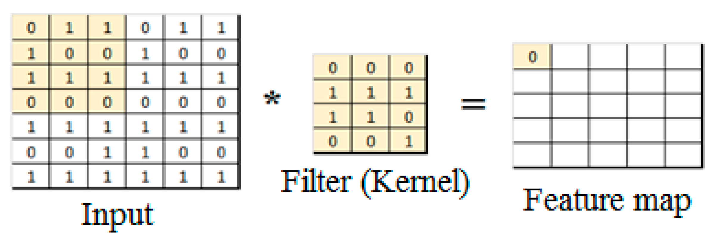
where $f\left[m,n\right]$ is the convolution filter, $g\left[u,v\right]$ is the input image, and $o\left[u,v\right]$ is the output feature map. The convolution operation is shown in Figure 2.

The convolution layers convolve the input images with a small grid shape called the kernel, or convolution filter, starting from the top left corner of the image, as shown in Figure 3. The convolution filter is used to extract important features from the input images that will help in classifying the images. The weights of the convolution filter are the most important in the CNN, which will be learned from the iterative nature of the backpropagation algorithm. Many filters will be used to extract as many features from the images as possible to be able to correctly classify the images.

The result of convolving the filter over the input image will produce a matrix that is called a feature map, where it can be considered as a reduced image that will be used instead of the original image in the subsequent layers. Many feature maps will be outputted from the filters used, every one of these maps will capture different features from each image, and these features will be used to correctly classify the images [19]. The backpropagation algorithm is used to tune the weights of the CNN by updating the weights from the last layers to the first. To protect the CNN from vanishing or exploding gradients, the weights of the CNN are initialized with a certain distribution and not from zero. The weights of the network can be transferred from one to another to avoid initializing the weights from scratch.

3.2. Transfer Learning

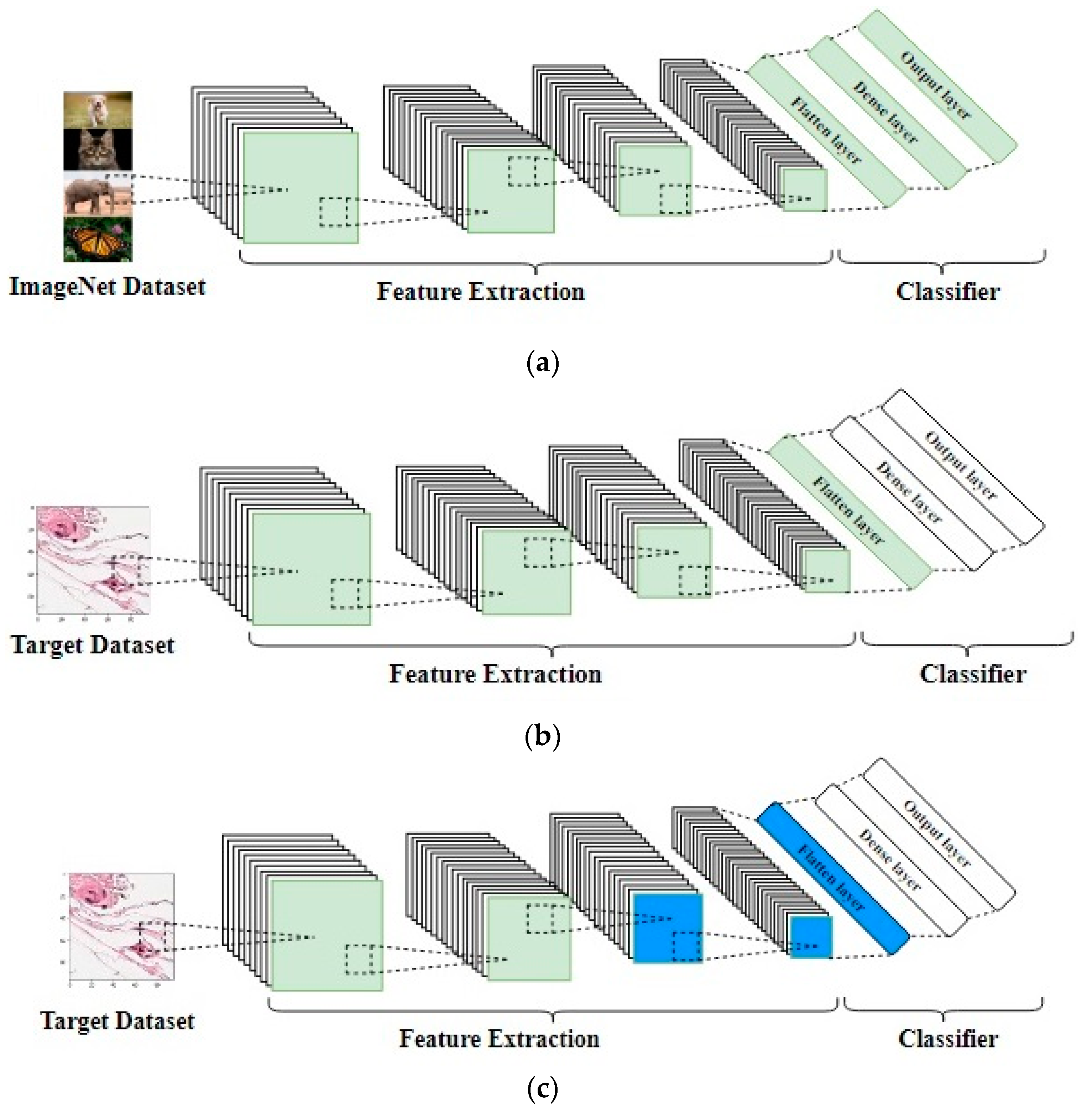
The source dataset is the dataset being used to train the CNN weights to be used for another target dataset; usually, the source dataset contains millions of images with thousands of classes, like the ImageNet dataset [32]. The following four techniques for transfer learning were introduced in the literature:

• The first technique is to freeze the source CNN’s weights (like ImageNet’s weights) and then remove the original fully connected layers and add another classifier, either a new fully connected layer or any machine learning classifier, like support vector machine (SVM), that is, to use the original weights for feature extraction.
• The second technique is to fine-tune the top layers of the source CNN with a very small learning rate and freeze the bottom layers, under the assumption that the bottom layers are very generic and can be used for any kind of image dataset [16].
• The third technique is to fine-tune the entire network’s weights using a very small learning rate to avoid losing the source weights, then remove the last fully connected layers, and add another layer to suit the target dataset.
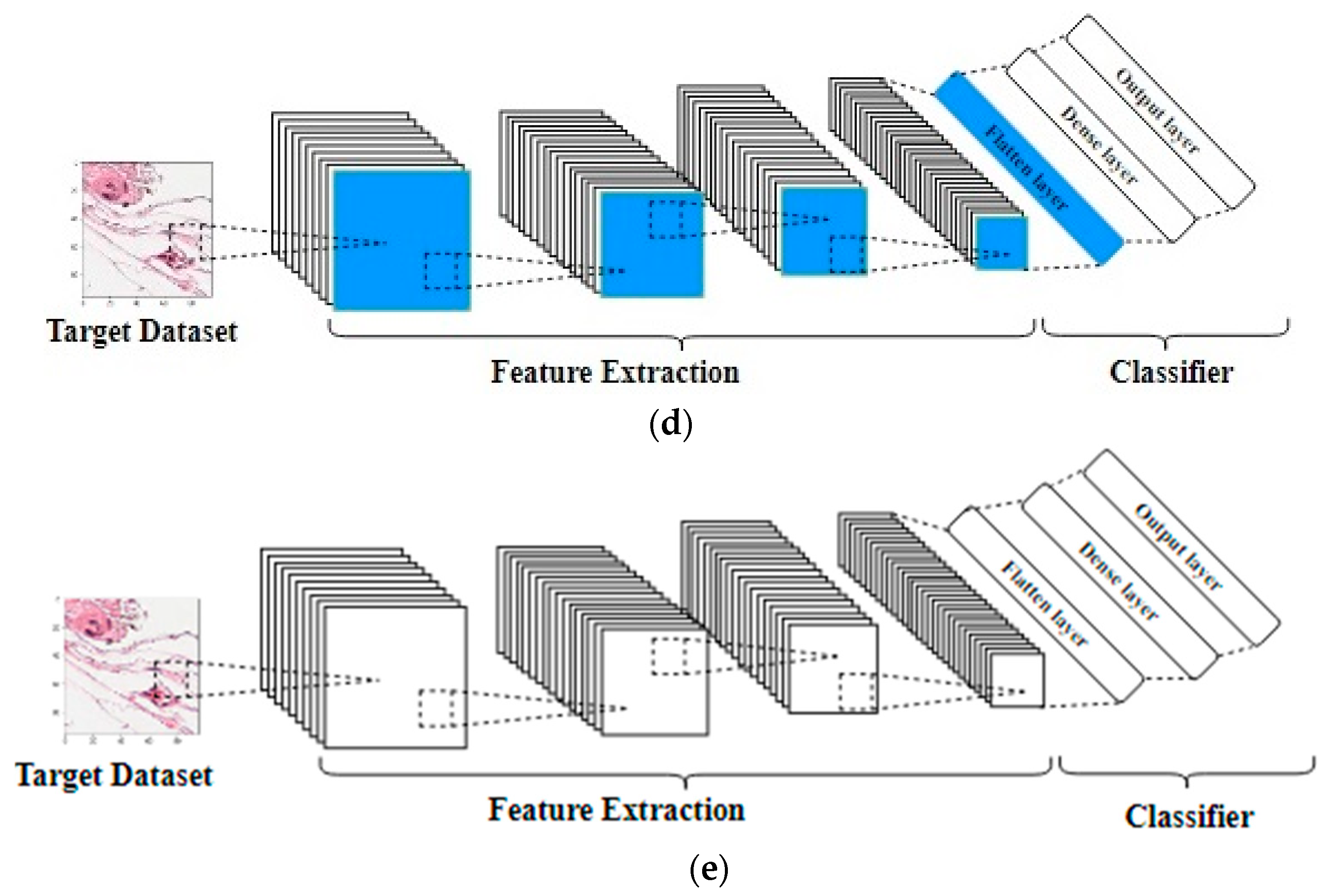
• The fourth technique is to use the CNN’s original architecture without importing any weights, that is, to initialize the weights from scratch. The point of this technique is using a well-known architecture that has been experimented with challenging datasets and proven to be good. Different transfer learning techniques are shown in Figure 4.

According to Pan and Yang [33], transfer learning in the image classification domain can be defined given the following parameters: $S:Source$, $\mathrm{T}:Target$, $n:Sourcedatasetsize$, $m:Targetdatasetsize$, $\varphi (.):$ objective function, $\mathcal{D}: Domain$, $ℱ:feature space$, $P\left(X\right):Marginal probability distribution$, and $learning samples: X=\left\{x_1,x_2, \dots ,x_n\right\}\in ℱ$, $\mathsf{{\rm Y}}: Label space$, $task: \mathsf{{\rm K}}=\left\{\mathsf{{\rm Y}},\varphi (.)\right\}$, $n\gg m$.

An image domain, $\mathcal{D},$ is defined as having two components: a feature space,$ℱ,$ and a probability distribution, $P\left(X\right)$:

$$\mathcal{D}=\left\{ℱ,P\left(X\right)\right\}$$

(5)

For a source domain, $S$, the dataset is $X_S=\left\{x_{S_1},x_{S_2},\dots ,x_{S_{\mathrm{n}}}\right\}\in {ℱ}_S.$

The source domain data can be denoted by:

$${\mathcal{D}}_S=\left\{\left(x_{S_1},y_{S_1}\right),\left(x_{S_2},y_{S_2}\right),\dots ,\left(x_{S_n},y_{S_n}\right)\right\}$$

(6)

where $x_{S_i}\in {ℱ}_S$ is the data instance, and $y_{S_i}\in {\mathsf{{\rm Y}}}_S$ is the corresponding class label.

For the target domain, $\mathsf{{\rm T}}$, the target domain can be denoted by:

$${\mathcal{D}}_{\mathsf{{\rm T}}}=\left\{\left(x_{{\mathsf{{\rm T}}}_m},y_{{\mathsf{{\rm T}}}_m}\right),\left(x_{{\mathsf{{\rm T}}}_m},y_{{\mathsf{{\rm T}}}_m}\right),\dots ,\left(x_{{\mathsf{{\rm T}}}_m},y_{{\mathsf{{\rm T}}}_m}\right)\right\}$$

(7)

where $x_{{\mathsf{{\rm T}}}_i}\in {ℱ}_{\mathsf{{\rm T}}}$ is the data instance, and $y_{{\mathsf{{\rm T}}}_i}\in {\mathsf{{\rm Y}}}_{\mathsf{{\rm T}}}$ is the corresponding class label.

A task, $\mathsf{{\rm K}},$ consists of two components: a label space, $\mathsf{{\rm Y}},$ and an objective function, $\varphi (.)$:

$$\mathsf{{\rm K}}=\left\{\mathsf{{\rm Y}},\varphi (.)\right\}$$

(8)

given a source domain, ${\mathcal{D}}_S$, and learning task, ${\mathsf{{\rm K}}}_{\mathrm{S}}$, a target domain, ${\mathcal{D}}_{\mathsf{{\rm T}}},$ and its learning task, ${\mathsf{{\rm K}}}_{\mathsf{{\rm T}}}$. Transfer learning aims to help improve the learning of the target predictive function ${\varphi }_{\mathsf{{\rm T}}}(.)$ in ${\mathsf{{\rm K}}}_{\mathsf{{\rm T}}}$ using the knowledge in ${\mathcal{D}}_S$ and ${\mathsf{{\rm K}}}_{\mathrm{S}}$, where ${\mathcal{D}}_{\mathrm{S}}\ne {\mathcal{D}}_{\mathsf{{\rm T}}}$ or ${\mathsf{{\rm K}}}_{\mathrm{S}}\ne {\mathsf{{\rm K}}}_{\mathsf{{\rm T}}}$. ${\mathcal{D}}_S$ represents the ImageNet dataset in our research and its learning task, ${\mathsf{{\rm K}}}_{\mathrm{S}}$, where ${\mathsf{{\rm K}}}_{\mathrm{S}}=\left\{{\mathsf{{\rm Y}}}_{\mathrm{S}},{\varphi }_S(.)\right\}$, given that ${\mathsf{{\rm Y}}}_{\mathrm{S}}$ is the source label space, and ${\varphi }_S(.)$ is the source predictive function that is used to map a new image $x_i$ to its label $y_i$. ${\mathcal{D}}_{\mathsf{{\rm T}}}$ represents the histopathology dataset in our research and its learning task, ${\mathsf{{\rm K}}}_{\mathsf{{\rm T}}}$, where ${\mathsf{{\rm K}}}_{\mathsf{{\rm T}}}=\left\{{\mathsf{{\rm Y}}}_{\mathsf{{\rm T}}},{\varphi }_{\mathsf{{\rm T}}}(.)\right\}$. As stated before, we want to enhance ${\varphi }_{\mathsf{{\rm T}}}(.)$ of the histopathology dataset, ${\mathcal{D}}_{\mathsf{{\rm T}}},$ using the ImageNet dataset, ${\mathcal{D}}_S,$ and its objective function, ${\varphi }_S(.)$ of ${\mathsf{{\rm K}}}_{\mathrm{S}}$.

3.3. CNN Architectures

Since AlexNet architecture achieved first place in the ImageNet challenge in 2012 with an error rate of 16%, many architectures were introduced using CNN to classify images. In 2014, VGG [24] architectures, which are considerably deeper than AlexNet architecture [12], were introduced, and in the same year, GoogLeNet architecture [28] was introduced as well, which is considered deeper and wider than AlexNet. Then, in 2015, ResNet architecture [29] was introduced and was deeper and contained the residual connection, and it was followed by DenseNet [26] in 2016. All of these state-of-the-art CNNs were trained on the ImageNet dataset, and their weights are publicly available. In this study, we decided to take into account three CNNs, namely, VGG16, VGG19, and InceptionV3 architectures. This choice is related to the fact that these three networks are the ones commonly used in the Kaggle competition associated with this dataset, and, even more important, they produced better performance with respect to the other competitors. Additionally, the choice of the architectures to be considered is not fundamental for developing our study that focuses on understanding whether fine-tuning is a suitable approach for analyzing the histopathology dataset at hand. Below, we briefly describe the CNNs used in this paper.

3.3.1. VGG Architectures

VGG architectures [24] were introduced by Oxford’s Visual Geometry Group in 2014 to participate in the ILSVRC competition, where it achieved a top-5 error rate of 7.3%. Two networks, namely VGG16 and VGG19, were introduced, and the only difference between the two networks is the number of convolution layers used. VGG16 consists of 13 convolution layers, and VGG19 consists of 16 convolution layers and so is considered deeper than VGG16. Instead of using a convolution layer with a large filter size, the authors concatenated two layers with a smaller filter size, which reduced the number of parameters by 28%. VGG networks consist of five convolution blocks, where the first two blocks consist of two convolution layers each with a filter size of $3\times 3$, the convolution layers in the first block have 64 filters each, while the convolution layers in the second block have 128 filters each. The third block in VGG16 consists of three convolution layers, and in VGG19, it has four convolution layers, all of the layers have 256 filters with size $3\times 3$. The fourth and fifth convolution blocks consist of three convolution layers in VGG16 and four convolution layers in VGG19, and all of the layers have 512 filters with size $3\times 3$. The five blocks are separated by a maximum pooling layer. Two fully connected layers are used as a classifier for the network with 4096 neurons. VGG16 has 138 million parameters with 23 layers’ depth, and VGG19 has 143 million parameters with 26 layers’ depth. VGG architectures are shown in Figure 5.

3.3.2. InceptionV3 Architecture

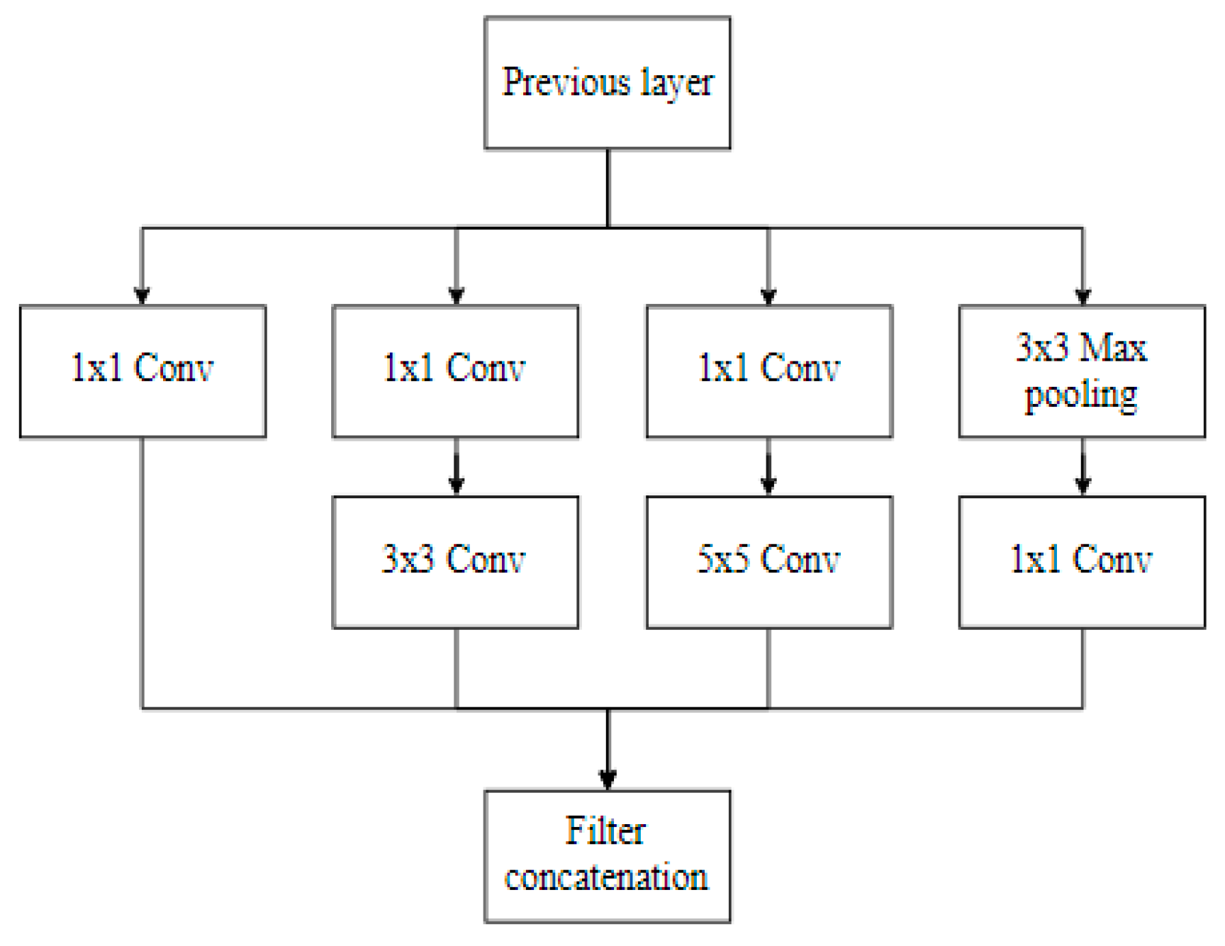
Inception architectures [28] were first introduced by the authors of Reference [34] in 2014 to participate in the ImageNet competition, winning first place with a top-5 error rate of 6.65%. They were designed under the hypothesis that different scales of the same object require different filter sizes to be observed correctly. The inception module starts with the same input, and then it will be split into different convolutional layers with different kernel sizes and one max pooling layer—these filters will be parallel to each other, and then the output will concatenate to a single layer. Having these layers parallel to each other and not subsequent like in VGG models will save a lot of memory and will increase the model’s capacity without increasing its depth. The inception module is shown in Figure 6. The version used in this paper is the third. Inception architecture consists of nine inception modules that are sequentially arranged. InceptionV3 architecture has 23.8 million parameters with 159 layers’ depth. Three filter sizes, namely $1\times 1$, $3\times 3,$ and $5\times 5$, are used in a single inception module; in the updated version, the authors replaced the $5\times 5$ with two $3\times 3$ convolution layers, influenced by Reference [24]. Inception architecture is shown in Figure 7.

3.4. Datasets Used

CNN algorithms, especially for the state-of-the-art architectures that are very deep, are very data-hungry and need hundreds of thousands of images to be accurately trained.

Two datasets were used in this study. One very large dataset—the ImageNet dataset, also called the original dataset—was used to train the CNN. The second dataset, the histopathology dataset, was the target dataset that we wanted to classify and that we used to fine-tune the weights that the ImageNet dataset learned. A brief description of both datasets follows.

3.4.1. ImageNet Dataset

In 2010, the ImageNet challenge [32], also known as the ImageNet Large-Scale Visual Recognition Challenge (ILSVRC), was introduced to push forward advances in the field of computer vision. ImageNet has millions of hand-labeled images using thousands of labels. The images are mainly everyday images, including animals, bridges, cars, and furniture, among others. A sample of the ImageNet dataset is shown in Figure 8.

3.4.2. PatchCamelyon Histopathology Dataset

The PatchCamelyon histopathology dataset [23,24] is a publicly available dataset that consists of 220,000 labeled images and 57,000 unlabeled images and contains a 60% positive class and a 40% negative class. The positive class means the middle region of the image ($32\times 32$) contains tumor tissue. The dataset has no duplicates. The test set can be evaluated on the Kaggle website, which produces the AUC of the ROC curve. A sample of the PatchCamelyon dataset is shown in Figure 9.

3.5. Performance Measures

Several performance measures have been introduced in the literature to assess the quality of the classifier. One of the most popular measures is the accuracy metric, wherein the classification domain can be defined as in Equation (9):

$$Accuracy=\frac{TP+TN}{TP+TN+FP+FN}$$

(9)

where $TP$ is the true positive, in which the positive class is predicted as positive, $TN$ is the true negative, in which the negative class was predicted as negative, $FP$ is the false positive, in which the negative class is incorrectly classified as positive, and $FN$ is the false negative, in which the positive class is incorrectly classified as negative. The main drawback of the accuracy metric is that it is only robust for balanced datasets; otherwise, it can be misleading. Another metric introduced was the sensitivity metric (also known as the true positive rate, or $TPR$), which is defined as in Equation (10):

$$Sensitivity=\frac{TP}{TP+FN}$$

(10)

which focuses on the positive classes and how accurately they were classified. Another metric, called the $Specificity$ (also known as the true negative rate, or $TNR$), was introduced to focus on the negative classes, which is defined as in Equation (11):

$$Specificity=\frac{TN}{TN+FP}$$

(11)

To combine the performance of both $Sensitivity$ and $Specificity$, a new metric called the receiver operating characteristic (ROC) curve was introduced. The ROC curve was developed during the Second World War [35]. It is a metric that is widely used to measure and visualize the classifier’s ability to distinguish between two classes [36]. The curve plots the $sensitivity$ against the $\left(1-specificity\right)$. To represent the area under the ROC curve, a metric called the area under the curve (AUC) is used. The AUC of the ROC curve ranges from 0.5 to 1, $0.5\le AUC\le 1$, where an AUC equal to 1 means that the classifier is able to distinguish between the positive and negative classes perfectly, and an AUC equal to 0.5 means that the classifier is just a random guess.

3.6. Measures to Avoid Overfitting

Due to the importance of any medical-images classifier, all of the measures necessary should be taken to ensure that the image classifier is robust against overfitting. Overfitting is defined as the model’s bad performance on the test dataset and perfect performance on the training dataset [37], which emphasizes the model’s generalizability. Many regularization techniques were introduced in the literature to overcome the problem of classifier overfitting by increasing the training error in exchange for decreasing the testing error, meaning to decrease the model variance by increasing the model bias [38]. The following measures aim to decrease errors in the test dataset irrespective of errors in the training dataset.

3.6.1. Early Stopping

A technique used to control the number of training epochs is early stopping. The model training will stop if the accuracy of the validation dataset does not change for a predefined number of epochs, meaning that the training will stop if the model starts to overfit the training dataset. Early stopping saves computational power and helps the CNN from overfitting the training dataset by doing useless epochs that will take a long time and decrease the network’s accuracy [38]. Early stopping can help optimize the epoch’s size hyperparameter by setting the epoch size too high and then letting early stopping automatically halt the training if no increase in accuracy occurs [39].

3.6.2. Best Model Saved

The model will be saved only if the accuracy in that epoch is larger than the largest accuracy achieved so far. The final model is the last saved one.

3.6.3. Dropout

Srivastava et al. [37] introduced dropout, which is considered a very important regularization technique that is usually used as an ensemble technique and is similar to a bagging algorithm [40,41]. Every single neuron that each layer is applied to has a probability,$p,$ to be dropped temporarily during training, so it can construct many networks from the same single network. Dropout can make a CNN very robust against overfitting [38].

3.6.4. Image Augmentation

One of the main methods to reduce overfitting is to have a huge training dataset to train the model on every single possible image, but practically, that is impossible, which is how augmentation was introduced. To increase the training dataset, image augmentation can be applied. Image augmentation is defined as an algorithm that can be used to create artificial images by modifying the original images through a series of transformations, rotations, and altered brightness, among other possible modifications.

4. Results

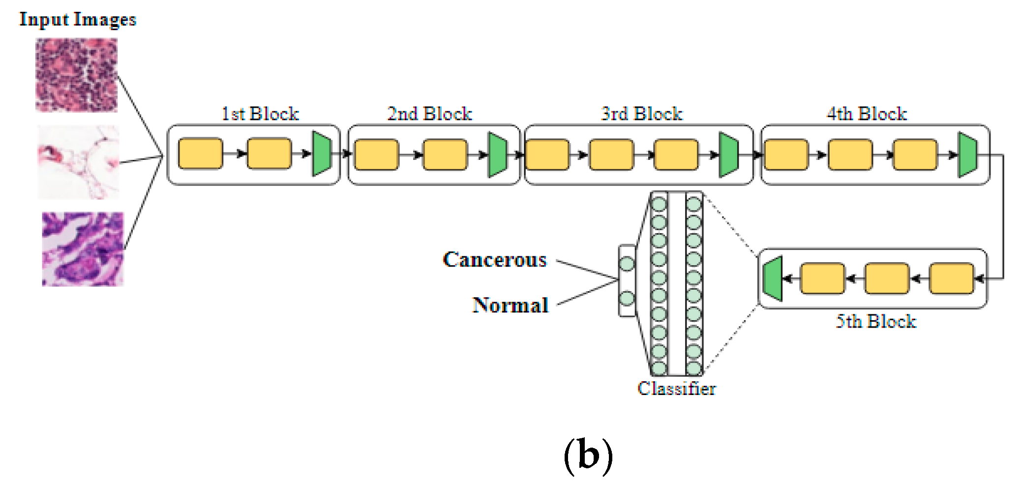
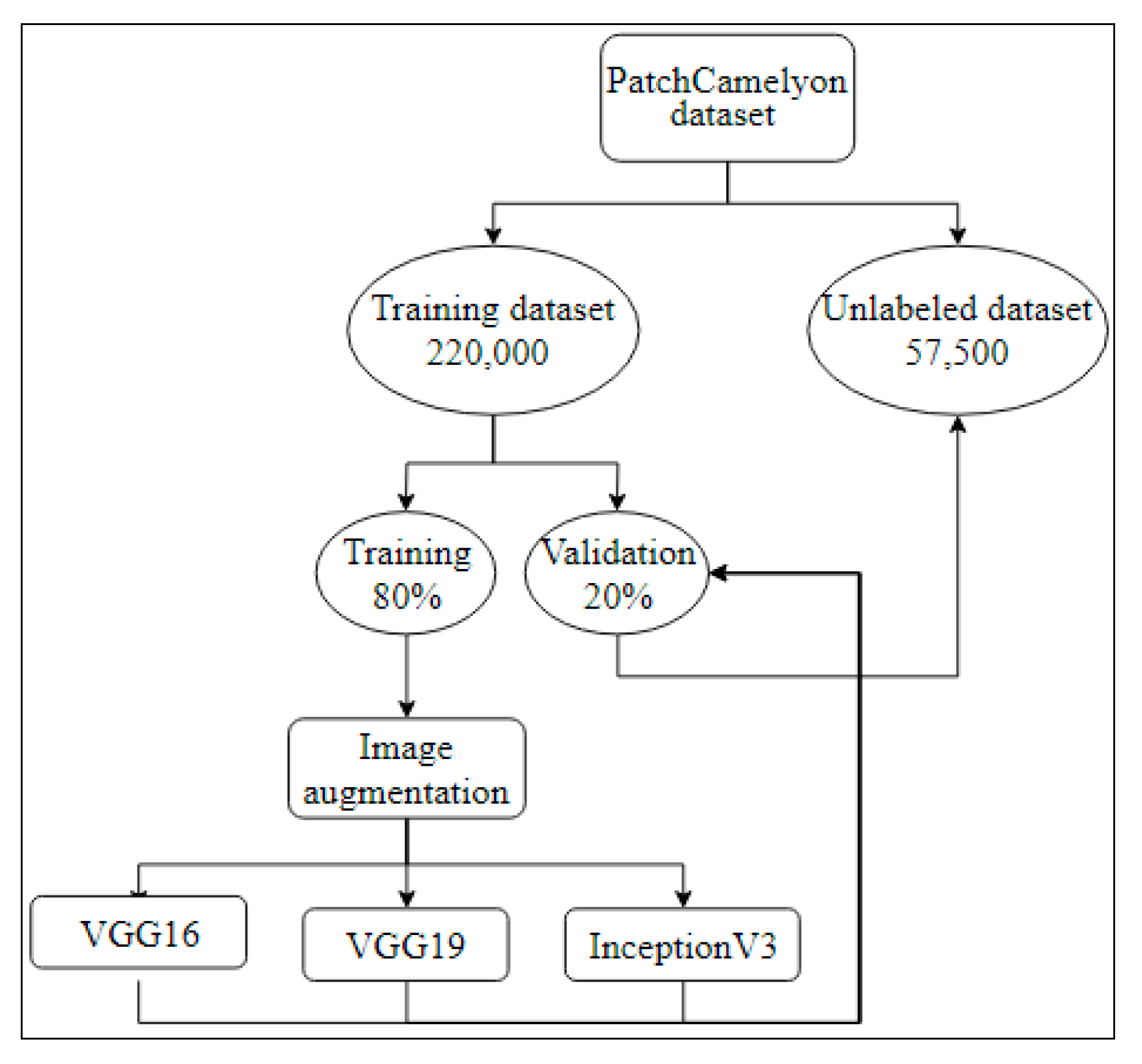
In this study, three CNN architectures were fine-tuned block-wise to determine the effect of fine-tuning each block on the generalizability of the network. The CNN architectures used were VGG16, VGG19, and InceptionV3. The original weights used were the ImageNet dataset weights. The dataset used was the publicly available PatchCamelyon dataset, and the dataset size was 220,000 labeled images for training, which consists of 60% of the positive class and 40% of the negative class. A separate 57,458 unlabeled images were provided to assess the classifier’s performance, and the results of classifying the test dataset were uploaded to the Kaggle website to determine the AUC of the ROC curve. In all of the experiments, the Keras library was used with Python. A schematic diagram of the proposed model is shown in Figure 10.

4.1. Experiment Parameters

Three CNN architectures were fine-tuned block-wise. The batch size used was 64, and three learning rates, namely ${10}^{-3}$, ${10}^{-4}$, and ${10}^{-5}$, were applied. The Adam optimizer [41] was used in all of the experiments. All of the images were kept at the original dimensions of $96\times 96pixels$. The original fully connected layers of the architectures were removed and replaced by a dropout layer with a probability of 50% to increase the network accuracy, and a new fully connected layer was used as a classifier. The training dataset was divided into two partitions: 80% and 20% for training and validation, respectively. To increase the size of the training dataset and to overcome the translation of the images, image augmentation was applied with the following parameters: horizontal and vertical flipping, $180°$ rotation, width and height shifting, and shearing and zooming. It is worth noting that image augmentation was applied to the training dataset only and not the validation dataset. The best model will be saved in every epoch, and the early stopping criteria of 10 epochs were applied.

Each CNN architecture was divided into blocks based on their design. For VGG networks, the blocks were divided based on the max-pooling layers, and for the InceptionV3 network, the blocks were defined based on the inception module, meaning that every inception module represents a block. VGG architectures have a total of 5 blocks, and the InceptionV3 network has 13 blocks. Each network was fine-tuned backward, meaning that the first block to be fine-tuned in the VGG networks was the 5th, and the first block to be fine-tuned in the InceptionV3 network was the 13th.

4.2. Experiment Results

The results of fine-tuning VGG16 with three different learning rates are shown in

Table 2. Results of the VGG16 architecture.

VGG16 Test AUC Results
Blocks	$\mathbf{LR}\mathbf{=}{\mathbf{10}}^{\mathbf{-}\mathbf{3}}$	$\mathbf{LR}\mathbf{=}{\mathbf{10}}^{\mathbf{-}\mathbf{4}}$	$\mathbf{LR}\mathbf{=}{\mathbf{10}}^{\mathbf{-}\mathbf{5}}$
Fine-Tuning 5th Block	0.9303	0.9260	0.9212
Fine-Tuning 4th Block	0.9398	0.9480	0.9382
Fine-Tuning 3rd Block	0.9364	0.9603	0.9475
Fine-Tuning 2nd Block	0.8893	0.9350	0.9384
Fine-Tuning ALL	0.9383	0.9310	0.9404

LR:learning rate.

. These results are the AUC of the ROC curve from the Kaggle website using the unlabeled dataset. The first block that was trained was the 5th block, and the results of the three learning rates are approximately the same, although the highest was with the ${10}^{-3}$ learning rate. The second block was the 4th, which was fine-tuned with the 5th layer, and the highest AUC obtained was by the ${10}^{-4}$ learning rate followed by the ${10}^{-3}$ and ${10}^{-5}$. The AUC results did increase by fine-tuning the 4th as well. The third experiment fine-tuned the blocks from the 5th to the 3rd, and the results obtained were higher than those of the previous two experiments. The highest was obtained by using the learning rate of ${10}^{-4}$. The fourth experiment fine-tuned the blocks from the 5th to the 2nd, and the results show that the accuracy started to decrease compared to the previous experiments. The fifth experiment fine-tuned the entire network, and the results were higher than the previous experiment but overall lower than the third experiment. Overall, the highest AUC was 96%, which was achieved by fine-tuning the last 3 blocks and using the ${10}^{-4}$ learning rate.

The results of fine-tuning the VGG19 network are shown in

Table 3. Results of the VGG19 architecture.

VGG19 Test AUC Results
Blocks	$\mathbf{LR}\mathbf{=}{\mathbf{10}}^{\mathbf{-}\mathbf{3}}$	$\mathbf{LR}\mathbf{=}{\mathbf{10}}^{\mathbf{-}\mathbf{4}}$	$\mathbf{LR}\mathbf{=}{\mathbf{10}}^{\mathbf{-}\mathbf{5}}$
Fine-Tuning 5th Block	0.9082	0.9028	0.9058
Fine-Tuning 4th Block	0.9268	0.9266	0.9235
Fine-Tuning 3rd Block	0.9087	0.9514	0.9440
Fine-Tuning 2nd Block	0.8377	0.9480	0.9254
Fine-Tuning ALL	0.8669	0.9427	0.9342

. The same procedure followed to fine-tune the VGG16 architecture was employed. According to the results reported in Table 3, it is possible to see that the highest AUC was obtained by fine-tuning the last three blocks, by freezing the other blocks, and with a learning rate of ${10}^{-4}$. A comparable performance is obtained with a learning rate of ${10}^{-5}$, while when a learning rate of ${10}^{-3}$ was used, the best performance was obtained by fine-tuning only the last two layers.

The results of fine-tuning the InceptionV3 architecture are shown in

Table 4. Results of the InceptionV3 architecture.

InceptionV3 Test AUC Results
Blocks	$\mathbf{LR}\mathbf{=}{\mathbf{10}}^{\mathbf{-}\mathbf{3}}$	$\mathbf{LR}\mathbf{=}{\mathbf{10}}^{\mathbf{-}\mathbf{4}}$	$\mathbf{LR}\mathbf{=}{\mathbf{10}}^{\mathbf{-}\mathbf{5}}$
Fine-Tuning 13th Block	0.8250	0.8220	0.8221
Fine-Tuning 12th Block	0.8514	0.8466	0.8446
Fine-Tuning 11th Block	0.8702	0.8446	0.8274
Fine-Tuning 10th Block	0.8648	0.8675	0.8429
Fine-Tuning 9th Block	0.8526	0.8816	0.8538
Fine-Tuning 8th Block	0.8574	0.8637	0.8469
Fine-Tuning 7th Block	0.8673	0.8429	0.8907
Fine-Tuning 6th Block	0.8923	0.8468	0.8950
Fine-Tuning 5th Block	0.8680	0.8730	0.8883
Fine-Tuning 4th Block	0.8483	0.8335	0.8686
Fine-Tuning 3rd Block	0.7715	0.8575	0.8641
Fine-Tuning 2nd Block	0.7175	0.8636	0.8785
Fine-Tuning ALL	0.8071	0.9058	0.9280

. The first experiment conducted using the InceptionV3 architecture was to freeze the entire network and fine-tune the last block (13th block) three times using three learning rates. The results were similar across the three learning rates, with the highest found by using the highest learning rate (${10}^{-3}$) and the lowest by using the medium learning rate (${10}^{-4}$). This procedure (that consists of fine-tuning the last n blocks and freezing the remaining blocks) was subsequently iterated for n in the range [2,13] and by considering at each iteration the three different learning rates. According to the results reported in Table 4, when considering a learning rate of ${10}^{-4} \mathrm{and} {10}^{-5}$, the best performance was obtained by fine-tuning the whole architecture (i.e., n = 13). On the other hand, with a learning rate of ${10}^{-3}$, the best performance was achieved by fine-tuning the last eight blocks (from block 6 to block 13), thus freezing the first five blocks.

To demonstrate the potential of the fine-tuning approach, we decided to compare its performance against the one obtained by using CNNs trained from scratch, specifically for the PatchCamelyon dataset.

The results of training the architectures from scratch are summarized in

Table 5. Results of different architectures trained from scratch.

Training from Scratch AUC Results
Networks	$\mathbf{LR}\mathbf{=}{\mathbf{10}}^{\mathbf{-}\mathbf{3}}$	$\mathbf{LR}\mathbf{=}{\mathbf{10}}^{\mathbf{-}\mathbf{4}}$	$\mathbf{LR}\mathbf{=}{\mathbf{10}}^{\mathbf{-}\mathbf{5}}$
VGG16	50%	90.55%	85.91%
VGG19	50%	84.77%	85.81%
InceptionV3	84.83%	87.93%	81.97%

. The first experiment was to train the three CNNs from scratch using three different learning rates. For VGG16 architecture, using the highest learning rate, the model did not converge at all for the stopping criteria we imposed. By using the medium learning rate, the model converged to an acceptable performance, which is the highest in this set of experiments but was lower than the result obtained by fine-tuning the network. The lowest learning rate did not produce satisfactory performance, and performs poorer with respect to the network trained by considering the medium learning rate value. Concerning the VGG19 architecture, it did behave the same as the VGG16 for the highest learning rate. The performance achieved using the medium learning rate value was lower than the one achieved by using the lowest learning rate. InceptionV3 architecture did converge for the smaller learning rate, and the best performance was obtained by using the medium learning rate value. Overall, training the network from scratch did not achieve better results than fine-tuning the network.

4.3. Experiment Results on a Different Histopathology Dataset

To corroborate the results obtained with the PatchCamelyon dataset and to strengthen our findings, we performed a second set of experiments using a different histopathology dataset, namely the BreakHis [18] dataset. The BreakHis dataset consists of 7909 images split into 2480 benign images and 5429 malignant images. To conduct our experiments, we split the dataset into 80% to train the model, 10% to validate the model during training, and 10% to test the model on unseen data. The early stopping was increased to 50 epochs because of the dataset size. The results of fine-tuning the BreakHis dataset using the VGG16 architecture are shown in

Table 6. Results of the VGG16 architecture using the BreakHis dataset.

VGG16 Test AUC Results
Blocks	$\mathbf{LR}\mathbf{=}{\mathbf{10}}^{\mathbf{-}\mathbf{3}}$	$\mathbf{LR}\mathbf{=}{\mathbf{10}}^{\mathbf{-}\mathbf{4}}$	$\mathbf{LR}\mathbf{=}{\mathbf{10}}^{\mathbf{-}\mathbf{5}}$
Fine-Tuning 5th Block	89.51%	91.76%	89.73%
Fine-Tuning 4th Block	88.50%	93.58%	94.03%
Fine-Tuning 3rd Block	86.21%	95.39%	95.76%
Fine-Tuning 2nd Block	86.79%	94.90%	93.91%
Fine-Tuning ALL	85.04%	92.47%	93.04%

, the results of using VGG19 are summarized in

Table 7. Results of the VGG19 architecture using the BreakHis dataset.

VGG19 Test AUC Results
Blocks	$\mathbf{LR}\mathbf{=}{\mathbf{10}}^{\mathbf{-}\mathbf{3}}$	$\mathbf{LR}\mathbf{=}{\mathbf{10}}^{\mathbf{-}\mathbf{4}}$	$\mathbf{LR}\mathbf{=}{\mathbf{10}}^{\mathbf{-}\mathbf{5}}$
Fine-Tuning 5th Block	89.14%	90.11%	88.68%
Fine-Tuning 4th Block	87.41%	91.67%	93.80%
Fine-Tuning 3rd Block	88.72%	96.79%	94.46%
Fine-Tuning 2nd Block	50.00%	95.46%	94.39%
Fine-Tuning ALL	87.29%	95.26%	94.30%

, and lastly, the results of using InceptionV3 are shown in

Table 8. Results of the InceptionV3 architecture using the BreakHis dataset.

InceptionV3 Test AUC Results
Blocks	$\mathbf{LR}\mathbf{=}{\mathbf{10}}^{\mathbf{-}\mathbf{3}}$	$\mathbf{LR}\mathbf{=}{\mathbf{10}}^{\mathbf{-}\mathbf{4}}$	$\mathbf{LR}\mathbf{=}{\mathbf{10}}^{\mathbf{-}\mathbf{5}}$
Fine-Tuning 13th Block	55.09%	55.80%	55.26%
Fine-Tuning 12th Block	61.61%	57.78%	53.45%
Fine-Tuning 11th Block	56.92%	56.74%	62.26%
Fine-Tuning 10th Block	61.58%	54.85%	53.54%
Fine-Tuning 9th Block	59.33%	55.35%	51.61%
Fine-Tuning 8th Block	51.26%	50.79%	50.63%
Fine-Tuning 7th Block	58.38%	51.62%	50.41%
Fine-Tuning 6th Block	56.63%	50.90%	53.38%
Fine-Tuning 5th Block	56.87%	50.52%	50.64%
Fine-Tuning 4th Block	57.46%	54.39%	50.57%
Fine-Tuning 3rd Block	52.00%	50.00%	50.00%
Fine-Tuning 2nd Block	50.00%	50.00%	52.00%
Fine-Tuning ALL	85.69%	94.72%	94.41%

.

As one can see from the analysis of Table 6, the results obtained by fine-tuning VGG16 using the BreakHis dataset match the results obtained on the PatchCamelyon dataset. In particular, fine-tuning the top layers and using the smallest learning rates of ${10}^{-4} \mathrm{and} {10}^{-5}$ did achieve the highest results. More in detail, with a learning rate of ${10}^{-3}$, the best performance was achieved by fine-tuning only the 5th block; with a learning rate of ${10}^{-4}$, the best performance was obtained through the fine-tuning of blocks from the 5th to the 3rd. Finally, the overall best performance was obtained with a learning rate of ${10}^{-5}$ and with the fine-tuning of blocks from the 5th to the 3rd.

Also, for the results obtained by fine-tuning VGG19 using the BreakHis dataset (Table 7), one can notice a similar behavior with respect to the analysis performed with the PatchCamelyon dataset: fine-tuning the top layers was sufficient to produce the best results, and the smaller learning rates yielded the best performance. More in detail, the best performance when considering a learning rate of ${10}^{-3}$ was obtained by only fine-tuning the 5th block. On the other hand, for both the remaining learning rates of ${10}^{-4}$ and ${10}^{-5}$, the best performance was achieved by fine-tuning blocks from the 5th to the 3rd.

Moving to the results obtained by fine-tuning InceptionV3 using the BreakHis dataset (Table 8), it is possible to observe the same pattern already discussed when we considered the PatchCamelyon dataset. In particular, with this architecture, fine-tuning the top layers did not achieve any satisfactory results. As for the PatchCamelyon dataset, the best results were achieved by fine-tuning the entire network.

Finally,

Table 9. Results of different architectures trained from scratch using the BreakHis dataset.

Training from Scratch AUC Results
Networks	$\mathbf{LR}\mathbf{=}{\mathbf{10}}^{\mathbf{-}\mathbf{3}}$	$\mathbf{LR}\mathbf{=}{\mathbf{10}}^{\mathbf{-}\mathbf{4}}$	$\mathbf{LR}\mathbf{=}{\mathbf{10}}^{\mathbf{-}\mathbf{5}}$
VGG16	50%	90.45%	86.51%
VGG19	50%	92.02%	85.65%
InceptionV3	88.32%	92.65%	81.64%

summarizes the results obtained by training the architectures from scratch on the BreakHis dataset. According to the results reported in Table 9, when considering the VGG16 architecture and the highest learning rate, the model did not converge at all for the stopping criteria we imposed. By using the medium learning rate, the model converged to an acceptable performance, which is the highest in this set of experiments but was lower than the result obtained by fine-tuning the network, it showed the lowest learning rate and performs poorer with respect to the network trained by considering the medium learning rate value. Focusing on the VGG19 architecture, it did behave the same as the VGG16 for all the considered learning rates. More in detail, the best performance was obtained with a learning rate of ${10}^{-4}$. Considering the InceptionV3 architecture, the results follow the same trend observed with the PatchCamelyon dataset. In particular, the training process did converge for the smaller learning rate, and the best performance was obtained by using the medium learning rate value. Similar to the results achieved on the PatchCamelyon dataset, Table 9 shows that training the network from scratch did not achieve better results than fine-tuning the network.

5. Discussion

Training a CNN for a medical dataset is a very difficult process because of the scarcity of medical images due to many reasons, and that is where transfer learning, in which the weights of another CNN that was trained on a different very large dataset can be used, can be very important for the medical field. This process of re-training the CNN on a target dataset is called fine-tuning. Fine-tuning the entire CNN is very time-consuming and does not guarantee the best performance. As pointed out by Yosinski et al. [16], for natural image datasets, the lower layers will learn more generic features, like circles and edges, that are common to mainly all image datasets, while the top layers can learn the very specific features of the original dataset.

In this study, we compared the block-wise effect of fine-tuning three state-of-the-art CNNs to classify the images of two histopathology datasets using three learning rates. The results of this study showed that fine-tuning the entire network did not give the best performance for the VGG architectures; instead, fine-tuning only the top blocks yielded the best performance. For the InceptionV3 architecture, fine-tuning the entire network did increase its performance. The main argument is in regard to the generalizability of the bottom layers, which can be used for any kind of dataset, meaning the weights of the bottom layer can be frozen.

The results show that the learning rate should be low in order to not to mess up the original weights of the network; also, making the learning rate very low will not increase the performance and will slow down the learning process. From the experiments, we found out that a 0.0001 learning rate achieved the perfect combination between training time and performance. Also, training the architectures from scratch was compared to fine-tuning techniques, and our results showed that training the network from scratch did not achieve higher results than fine-tuning the network. Also, using higher learning rates made shallow architectures like VGGs very unstable and prevented them from convergence.

Comparing the results that we obtained with those obtained by other authors was difficult because the other methods used either different evaluation criteria or different datasets. For example, Kassani et al. [19] used the PatchCamelyon dataset as well and achieved accuracy of 94.64%, but the authors did not explain how they used transfer learning or whether they fine-tuned the entire networks or not, did not state the size of their test dataset, and did not state whether or not they used the unlabeled dataset. The highest result we achieved was done by fine-tuning the VGG16 top blocks to the 3rd block, and it was an AUC of 96%. As stated earlier, the results were obtained by predicting the unlabeled test dataset and submitting that to the Kaggle platform; therefore, all of our results are in the AUC of the ROC curve because that is the criteria used by Kaggle to assess the performance of the classifier.

As for other authors who used different histopathology datasets, Ahmad et al. [31] reported an accuracy of 85% for the BioImaging dataset using a fine-tuned ResNet architecture, but the authors did not report the transfer learning technique they used to achieve this result. Sharma et al. [17] achieved an accuracy of 92.6% and an AUC of 95.65% by using the VGG16 network with logistic regression as a classifier, but the authors did not investigate the role each block plays in the network performance. Further, the authors split the dataset into two partitions to assess its accuracy using three heuristics: the first split the dataset into 90% and 10%, the second split the dataset into 80% and 20%, and the last split the dataset into 70% and 30%. The authors did not use any validation algorithms like k-fold validation. The results of the three heuristics are approximately similar to each other. Deniz et al. [30] compared fine-tuning with feature extraction for the BreakHis dataset, and the authors reported that the fine-tuned AlexNet outperformed the VGG16 with SVM as a feature extractor. We can conclude from these studies that fine-tuning a CNN outperformed other techniques and that encouraged us to investigate the role of each block to further increase the CNN’s performance.

6. Conclusions

This paper concentrated on the impact of CNN architecture depth while fine-tuning the network. The architectures used, namely VGG16, VGG19, and InceptionV3, were pre-trained on the ImageNet dataset. All of the networks were fine-tuned on two different histopathology datasets to determine the effect of each block on the generalizability of the network. Three learning rates were used with an Adam optimizer to determine the effect of learning on the performance as well. Our results suggest that for shallow networks like VGG, fine-tuning the top layers can be sufficient to obtain decent results, while for deep networks like InceptionV3, fine-tuning the entire network can yield better results. In all cases, the low learning rate is highly recommended when fine-tuning the network in order to not mess up the original weights. Our recommendation in the case of a scarcity of images is that fine-tuning a pre-trained CNN can be a feasible option. The conclusions drawn from this study, concerning fine-tuning, refer to the particular application at hand. To further strengthen our finding and to draw more general conclusions that could be applied independently from the applicative domain, it would have been necessary to perform a study that involved dozens and dozens of datasets over different domains.

In future work, we will use different optimizers to detect the effect of the optimizers as well and will use different datasets, including non-medical ones, to detect the block-wise effect of fine-tuning CNNs.

References

1. Gurcan, M.N.; Boucheron, L.E.; Can, A.; Madabhushi, A.; Rajpoot, N.; Yener, B. Histopathological Image Analysis: A Review. IEEE Rev. Biomed. Eng. 2009, 2, 147–171. [Google Scholar] [CrossRef] [PubMed] [Green Version]
2. Metter, D.M.; Colgan, T.J.; Leung, S.T.; Timmons, C.F.; Park, J.Y. Trends in the US and Canadian Pathologist Workforces from 2007 to 2017. JAMA Netw. Open 2019, 2, e194337. [Google Scholar] [CrossRef] [PubMed] [Green Version]
3. LeCun, Y.; Boser, B.; Denker, J.S.; Henderson, D.; Howard, R.E.; Hubbard, W.; Jackel, L.D. Backpropagation Applied to Handwritten Zip Code Recognition. Neural Comput. 1989, 1, 541–551. [Google Scholar] [CrossRef]
4. Mohammadian, S.; Karsaz, A.; Roshan, Y.M. Comparative Study of Fine-Tuning of Pre-Trained Convolutional Neural Networks for Diabetic Retinopathy Screening. In Proceedings of the 2017 24th National and 2nd International Iranian Conference on Biomedical Engineering (ICBME), Tehran, Iran, 30 November–1 December 2017; pp. 1–6. [Google Scholar] [CrossRef]
5. Prentašić, P.; Lončarić, S. Detection of exudates in fundus photographs using convolutional neural networks. In Proceedings of the 2015 9th International Symposium on Image and Signal Processing and Analysis (ISPA), Zagreb, Croatia, 7–9 September 2015; pp. 188–192. [Google Scholar] [CrossRef]
6. Khan, N.; Abraham, N.; Hon, M. Transfer learning with intelligent training data selection for prediction of Alzheimer’s Disease. IEEE Access 2019, 7, 72726–72735. [Google Scholar] [CrossRef]
7. Farooq, A.; Anwar, S.M.; Awais, M.; Rehman, S. A deep CNN based multi-class classification of Alzheimer’s disease using MRI. In Proceedings of the 2017 IEEE International Conference on Imaging Systems and Techniques (IST), Beijing, China, 18–20 October 2017; pp. 1–6. [Google Scholar] [CrossRef]
8. Hosny, K.M.; Kassem, M.; Foaud, M.M. Classification of skin lesions using transfer learning and augmentation with Alex-net. PLoS ONE 2019, 14, e0217293. [Google Scholar] [CrossRef] [Green Version]
9. Harangi, B. Skin lesion classification with ensembles of deep convolutional neural networks. J. Biomed. Inform. 2018, 86, 25–32. [Google Scholar] [CrossRef]
10. Fukushima, K. Neocognitron: A self-organizing neural network model for a mechanism of pattern recognition unaffected by shift in position. Boil. Cybern. 1980, 36, 193–202. [Google Scholar] [CrossRef]
11. Hubel, D.H.; Wiesel, T.N. Ferrier lecture. Functional architecture of macaque monkey visual cortex. Proc. R. Soc. Lond. Ser. B 1977, 198, 1–59. [Google Scholar]
12. Krizhevsky, A.; Sutskever, I.; Hinton, G.E. ImageNet Classification with Deep Convolutional Neural Networks. Neural Inf. Process. Syst. 2012, 25. [Google Scholar] [CrossRef]
13. Russakovsky, O.; Deng, J.; Su, H.; Krause, J.; Satheesh, S.; Ma, S.; Huang, Z.; Karpathy, A.; Khosla, A.; Bernstein, M.; et al. ImageNet Large Scale Visual Recognition Challenge. Int. J. Comput. Vis. 2015, 115, 211–252. [Google Scholar] [CrossRef] [Green Version]
14. Tajbakhsh, N.; Shin, J.Y.; Gurudu, S.R.; Hurst, R.T.; Kendall, C.B.; Gotway, M.B.; Liang, J. Convolutional Neural Networks for Medical Image Analysis: Full Training or Fine Tuning? IEEE Trans. Med. Imaging 2016, 35, 1299–1312. [Google Scholar] [CrossRef] [Green Version]
15. Chollet, F. Deep Learning with Python, 1st ed.; Manning Publications Co.: Greenwich, CT, USA, 2017. [Google Scholar]
16. Yosinski, J.; Clune, J.; Bengio, Y.; Lipson, H. How transferable are features in deep neural networks? In Proceedings of the Advances in Neural Information Processing Systems 27, Montreal, QC, Canada, 8–13 December 2014; pp. 3320–3328. [Google Scholar]
17. Sharma, S.; Mehra, D.R. Breast cancer histology images classification: Training from scratch or transfer learning? ICT Express 2018, 4, 247–254. [Google Scholar] [CrossRef]
18. Spanhol, F.; Oliveira, L.S.; Petitjean, C.; Heutte, L. A Dataset for Breast Cancer Histopathological Image Classification. IEEE Trans. Biomed. Eng. 2015, 63, 1455–1462. [Google Scholar] [CrossRef]
19. Kassani, S.H.; Kassani, P.H.; Wesolowski, M.J.; Schneider, K.A.; Deters, R. Classification of Histopathological Biopsy Images Using Ensemble of Deep Learning Networks. arXiv 2019, arXiv:1909.11870. [Google Scholar]
20. Veeling, B.S.; Linmans, J.; Winkens, J.; Cohen, T.; Welling, M. Rotation Equivariant CNNs for Digital Pathology. In Medical Image Computing and Computer Assisted Intervention—MICCAI 2018; Springer: Berlin/Heidelberg, Germany, 2018; pp. 210–218. [Google Scholar]
21. Bejnordi, B.E.; Veta, M.; Van Diest, P.J.; Van Ginneken, B.; Karssemeijer, N.; Litjens, G.; Van Der Laak, J.A.W.M. Diagnostic Assessment of Deep Learning Algorithms for Detection of Lymph Node Metastases in Women with Breast Cancer. JAMA 2017, 318, 2199–2210. [Google Scholar] [CrossRef] [PubMed]
22. Aresta, G.; Araújo, T.; Kwok, S.; Chennamsetty, S.S.; Safwan, M.; Alex, V.; Marami, B.; Prastawa, M.; Chan, M.; Donovan, M.; et al. BACH: Grand challenge on breast cancer histology images. Med. Image Anal. 2019, 56, 122–139. [Google Scholar] [CrossRef]
23. BioImaging Dataset. 2015. Available online: http://www.bioimaging2015.ineb.up.pt/dataset.html (accessed on 1 December 2019).
24. Simonyan, K.; Zisserman, A. Very Deep Convolutional Networks for Large-Scale Image Recognition. arXiv 2014, arXiv:1409.1556. [Google Scholar]
25. Howard, A.G.; Zhu, M.; Chen, B.; Kalenichenko, D.; Wang, W.; Weyand, T.; Andreetto, M.; Adam, H. MobileNets: Efficient Convolutional Neural Networks for Mobile Vision Applications. arXiv 2017, arXiv:1704.04861. [Google Scholar]
26. Huang, G.; Liu, Z.; Van Der Maaten, L.; Weinberger, K.Q. Densely Connected Convolutional Networks. In Proceedings of the 2017 IEEE Conference on Computer Vision and Pattern Recognition (CVPR), Honolulu, HI, USA, 21–26 July 2017; pp. 2261–2269. [Google Scholar] [CrossRef] [Green Version]
27. Vesal, S.; Ravikumar, N.; Davari, A.; Ellmann, S.; Maier, A. Classification of Breast Cancer Histology Images Using Transfer Learning; Image Analysis and Recognition; Springer Nature: Berlin, Germay, 2018. [Google Scholar]
28. Szegedy, C.; Vanhoucke, V.; Ioffe, S.; Shlens, J.; Wojna, Z. Rethinking the Inception Architecture for Computer Vision. In Proceedings of the 2016 IEEE Conference on Computer Vision and Pattern Recognition (CVPR), Las Vegas, NV, USA, 27–30 June 2016; pp. 2818–2826. [Google Scholar] [CrossRef] [Green Version]
29. He, K.; Zhang, X.; Ren, S.; Sun, J. Deep Residual Learning for Image Recognition. In Proceedings of the 2016 IEEE Conference on Computer Vision and Pattern Recognition (CVPR), Las Vegas, NV, USA, 27–30 June 2016; pp. 770–778. [Google Scholar] [CrossRef] [Green Version]
30. Deniz, E.; Sengur, A.; Kadiroğlu, Z.; Guo, Y.; Bajaj, V.; Budak, Ü. Transfer learning based histopathologic image classification for breast cancer detection. Health Inf. Sci. Syst. 2018, 6, 18. [Google Scholar] [CrossRef]
31. Ahmad, H.M.; Ghuffar, S.; Khurshid, K. Classification of Breast Cancer Histology Images Using Transfer Learning. In Proceedings of the IEEE International Bhurban Conference on Applied Sciences and Technology (IBCAST), Islamabad, Pakistan, 8–12 January 2019; Volume 16. [Google Scholar] [CrossRef]
32. Deng, J.; Dong, W.; Socher, R.; Li, L.-J.; Li, K.; Li, F.-F. ImageNet: A large-scale hierarchical image database. In Proceedings of the 2009 IEEE Conference on Computer Vision and Pattern Recognition, Miami, FL, USA, 20–25 June 2009; pp. 248–255. [Google Scholar] [CrossRef] [Green Version]
33. Pan, S.J.; Yang, Q. A Survey on Transfer Learning. IEEE Trans. Knowl. Data Eng. 2010, 22, 1345–1359. [Google Scholar] [CrossRef]
34. Szegedy, C.; Liu, W.; Jia, Y.; Sermanet, P.; Reed, S.; Anguelov, D.; Erhan, D.; Vanhoucke, V.; Rabinovich, A. Going deeper with convolutions. In Proceedings of the 2015 IEEE Conference on Computer Vision and Pattern Recognition (CVPR), Boston, MA, USA, 7–12 June 2015; pp. 1–9. [Google Scholar] [CrossRef] [Green Version]
35. AnaSubtil, L.G.; Oliveira, M.; Bermudez, P. ROC curve estimation: An overview. Revstat Stat. J. 2014, 12, 1–20. [Google Scholar]
36. Fawcett, T. An introduction to ROC analysis. Pattern Recognit. Lett. 2006, 27, 861–874. [Google Scholar] [CrossRef]
37. Srivastava, N.; Hinton, G.; Krizhevsky, A.; Sutskever, I.; Salakhutdinov, R. Dropout: A Simple Way to Prevent Neural Networks from Overfitting. J. Mach. Learn. Res. 2014, 15, 1929–1958. [Google Scholar]
38. Goodfellow, I.; Bengio, Y.; Courville, A. Deep Learning; The MIT Press: Cambridge, MA, USA, 2016. [Google Scholar]
39. Bengio, Y. Practical recommendations for gradient-based training of deep architectures. In Neural Networks: Tricks of the Trade; Springer: Berlin/Heidelberg, Germany, 2012; Volume 7700, pp. 437–478. [Google Scholar]
40. Breiman, L. Bagging Predictors. Mach. Learn. 1996, 24, 123–140. [Google Scholar] [CrossRef] [Green Version]
41. Kingma, D.; Ba, J. Adam: A Method for Stochastic Optimization. arXiv 2014, arXiv:1412.6980. [Google Scholar]
Figure 1. Convolutional neural network (CNN) diagram.
Applsci 10 03359 g001
Figure 2. Convolutional operation.
Applsci 10 03359 g002
Figure 3. Convolution filter to extract features.
Applsci 10 03359 g003
Figure 4. This figure shows different transfer learning techniques: (a) a generic CNN trained on ImageNet dataset, (b) the first technique, in which the source weights are fixed and the original classifier layers will be replaced by new layers to suit the target dataset, (c) the second technique, in which the top layers will be fine-tuned, the weights of the bottom layer will be fixed, and the last fully connected layers will be replaced, (d) the third technique, in which the original classifier layers will be replaced and the entire network will be fine-tuned, and (e) the fourth technique, in which the original architecture will be used without any weights. The green color represents the weights learned from the ImageNet dataset, the blue color represents the fine-tuning of the ImageNet weights using the target dataset, and the white color means that the weights will be initialized from scratch.
Applsci 10 03359 g004aApplsci 10 03359 g004b
Figure 5. This figure shows VGG network architectures: (a) VGG19 architecture and (b) VGG16 architecture.
Applsci 10 03359 g005aApplsci 10 03359 g005b
Figure 6. The inception module.
Applsci 10 03359 g006
Figure 7. The Inception V3 architecture.
Applsci 10 03359 g007
Figure 8. A sample of the ImageNet dataset.
Applsci 10 03359 g008
Figure 9. A sample of the PatchCamelyon dataset.
Applsci 10 03359 g009
Figure 10. A schematic diagram of the proposed model.
Applsci 10 03359 g010