Decentralized Optimization of Electricity-Natural Gas Flow Considering Dynamic Characteristics of Networks

Abstract

The interconnection of power and natural gas systems can improve the flexibility of system operation and the capacity of renewable energy consumption. It is necessary to consider the interaction between both, and carry out collaborative optimization of energy flow. For space-time related line packs, this paper studies the optimal multi-energy flow (OMEF) model of an integrated electricity-gas system, taking into account the dynamic characteristics of a natural gas system. Besides, in order to avoid the problem of large data collection in centralized algorithms and consider the characteristics of decentralized autonomous decision-making for each subsystem, this paper proposes a decentralized algorithm for the OMEF problem. This algorithm transforms the original non-convex OMEF problem into an iterative convex programming problem through penalty convex-concave procedure (PCCP), and then, uses the alternating direction method of multipliers (ADMM) algorithm at each iteration of PCCP to develop a decentralized collaborative optimization of power flow and natural gas flow. Finally, numerical simulations verify the effectiveness and accuracy of the algorithm proposed in this paper, and analyze the effects of dynamic characteristics of networks on system operation.

1. Introduction

With the energy crisis and global environmental issues becoming increasingly prominent, it is necessary to develop multi-energy complementarity and optimization of an integrated energy system to achieve low-carbon environmental operations [1]. The development of gas turbines [2] and power to gas (P2G) [3] has enabled a bidirectional energy flow between the power system and the natural gas system, which promotes the formation of integrated electricity-gas system (IEGS). As an important part of Energy Internet, IEGS is also the development direction of Smart Grid [4,5,6].

Recently, a considerable amount of research has been made on the optimization of IEGS [7,8,9,10,11,12,13,14,15]. A unified modeling framework for IEGS is proposed in [7]. Based on this model, the effect of a natural gas system on the operation of a power system in accordance with the security-constrained unit commitment is discussed. Based on mixed integer linear programming, paper [8] presents an integrated electricity-gas system model that can be used to research interdependencies and identify critical vulnerabilities. Paper [9] studies the electricity and steady-state natural gas flow. The above studies are directed at steady-state models. However, for the network characteristics of IEGS, different systems have different dynamic characteristics. Natural gas flow operates at slower rates than electric power. Some natural gas is stored in the pipeline, which is called the “line pack”. In order to describe the natural gas network model more accurately, it is necessary to consider the line pack. Papers [10,11,12,13] have proved the improvement effect of the management of IEGS on the flexibility and reliability by considering the line pack. Paper [10] proposes a mixed-integer linear programing (MILP) model that takes into account the dynamic characteristics of natural gas system to solve the optimal energy flow of IEGS. Considering the different response times of the gas and power systems, the dynamic optimal energy flow in the IEGS is discussed in [11,12]. Paper [13] establishes the optimal operation model of IES considering heat-gas dynamic characteristics and demonstrates the efficiency of the proposed method for improving the flexibility and economy of IES operation. Paper [14] proposes a hybrid multi-energy load forecasting (MELF) method for IEGS considering temporal dynamic and coupling characteristics. An interdependent electricity-natural gas system considering electricity grid steady-state and gas network dynamics is established in [15]. Based on the model, the effect of P2Gs and gas turbines on the operational economics and robustness of IEGS is discussed.

On the other hand, in the above research works, the optimal scheduling model is mainly solved by centralized algorithms, which requires a central computer to collect global data to perform centralized calculations and control. However, the power and natural gas systems belong to different interest groups, and the information and operating conditions of each system have a certain privacy, which makes centralized optimization scheduling no longer applicable. Decentralized algorithms can solve the abovementioned limitations of centralized algorithms and can reduce the amount of information transmitted and reduce the risk of information blocking. Therefore, in the background of the energy internet, it is necessary to research the decentralized OMEF of IEGS [16,17,18].

However, the OMEF problem is a non-convex optimization problem that is difficult to solve. The inherent non-convexity makes traditional decentralized algorithms unable to converge or obtain ideal results. The non-convexity of the OMEF problem comes from the second-order power flow equation and natural gas flow equation. To handle this issue, extensive optimization methods have been presented. There are two main convex methods for the second-order power flow equation. One is the linear DC power flow model [19], the other is the second-order cone relaxation for the radial grid model [20]. However, both methods have their own limitations. For the non-convex natural gas flow equation, piecewise linearization techniques are used to deal with it. However, piecewise linearization models limit gas flow directions [21,22]. Some researchers have proposed the mixed integer second-order cone relaxation technique to convexize the equation [17,23,24], but a large number of integer variables make the model complicated. The above research works have certain limitations on the treatment of non-convex terms in the OMEF problem.

Aiming at the above problems, this paper proposes a decentralized optimization algorithm for OMEF based on PCCP-ADMM, which has the following main novelty and contribution.

• The non-convex OMEF problem is transformed into a convex optimization problem by PCCP. For the power system model, based on the paper [25], this paper studies the method of convexity of the second-order power flow equation in the multi-period OMEF model, which effectively retains all the electrical quantities and is suitable for any topology. For the natural gas system model considering the dynamic characteristics, the positive and negative natural gas flow are introduced into the model, and the PCCP method is used to convexize the flow equation, which can efficiently solve the natural gas system model.
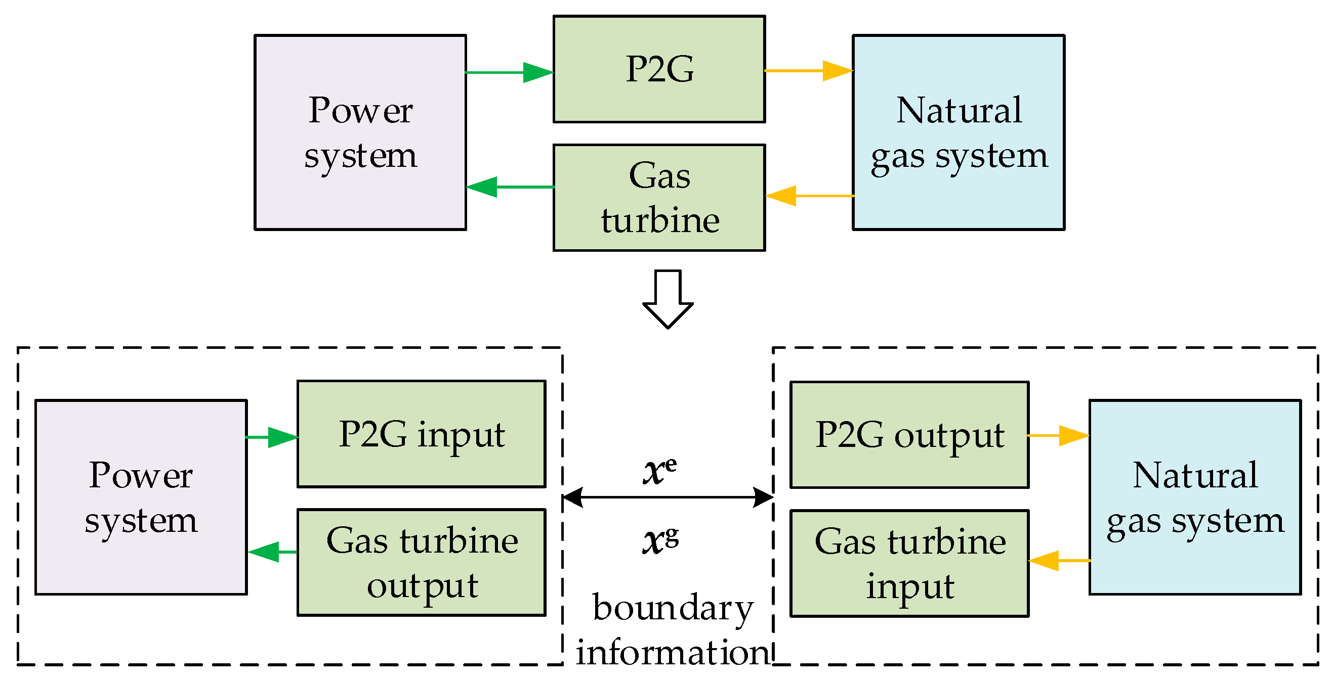
• The decentralized optimization process is based on the obtained convex OMEF model. At each iteration of the PCCP, ADMM is used to establish and solve the decentralized OMEF problem of IEGS. During the solution process, each system only needs to exchange a small amount of boundary information, which achieves independent optimization and partition coordination. The solution process ensures the privacy and security of each system information. Finally, testing IEGS combined with an IEEE 39-bus power system and a Belgian 20-bus natural gas system is used to verify the proposed algorithm and can effectively solve the decentralized OMEF problem.

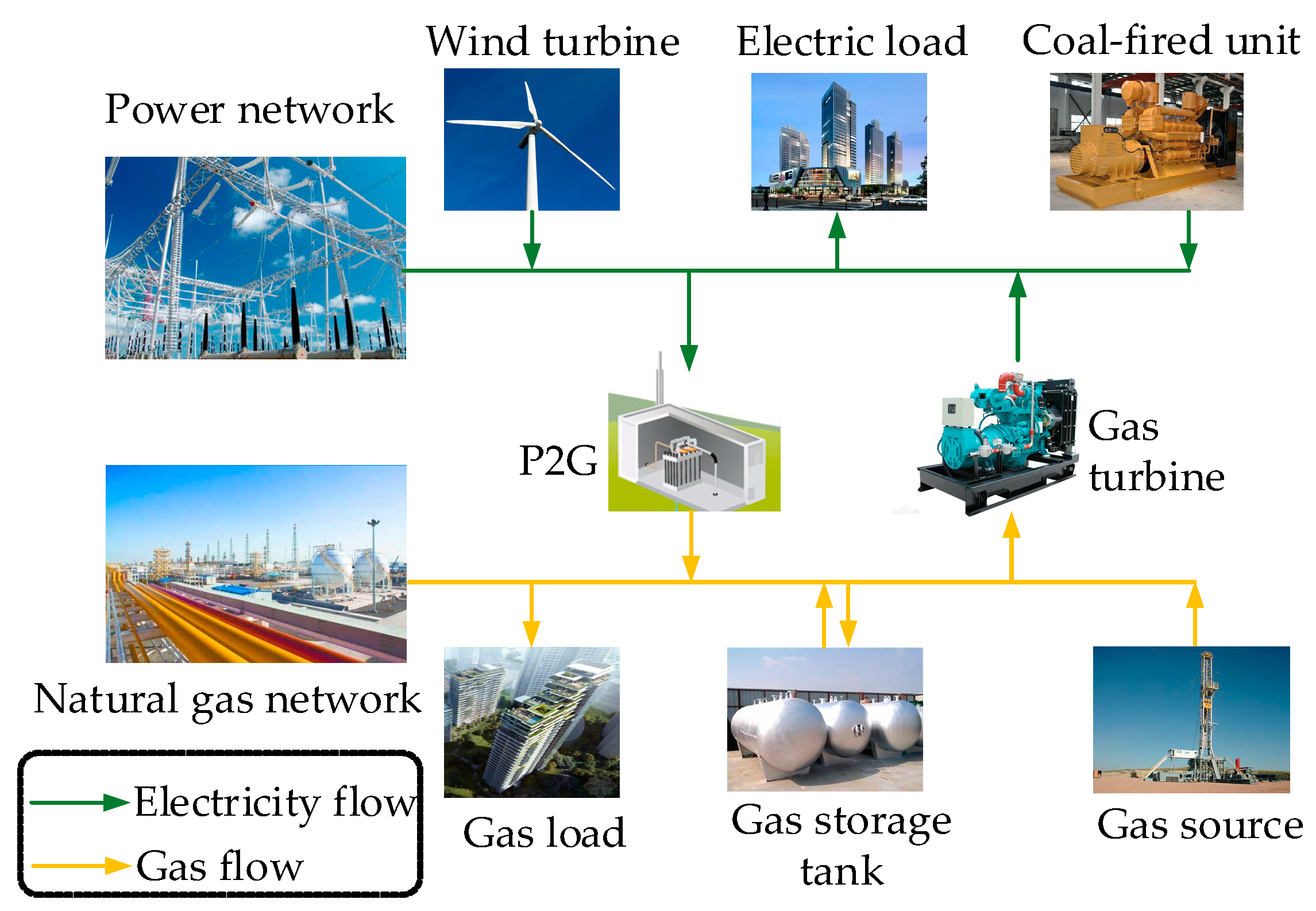
2. Modeling for OMEF

Due to the non-convexity of the OMEF model, the OMEF problem of IEGS is a difficult non-convex optimization problem. In this part, the OMEF is modeled and the non-convex term is effectively processed with PCCP. The OMEF problem is transformed into a convex optimization problem. The IEGS studied in this paper consists of a power network and a natural gas network. The power and natural gas systems are interconnected through P2Gs and gas turbines, as shown in Figure 1.

2.1. Power System

2.1.1. Modeling for Power System

(1) Power balance

$$P_{\mathrm{G},i,t}-P_{\mathrm{D},i,t}-P_{\mathrm{P}2\mathrm{G},i,t}=g_{ii}{V}_{i,t}^2+{\displaystyle \sum _{j\in i,j\ne i}{P}_{ij,t}}$$

(1)

$$Q_{\mathrm{G},i,t}-Q_{\mathrm{D},i,t}=-b_{ii}{V}_{i,t}^2+{\displaystyle \sum _{j\in i,j\ne i}{Q}_{ij,t}}$$

(2)

$$P_{ij,t}=g_{ij}{V}_{i,t}^2-g_{ij}{V}_{i,t}{V}_{j,t}\cos {\theta }_{ij,t}-b_{ij}{V}_{i,t}{V}_{j,t}\sin {\theta }_{ij,t}$$

(3)

$$Q_{ij,t}=-b_{ij}{V}_{i,t}^2-g_{ij}{V}_{i,t}{V}_{j,t}\sin {\theta }_{ij,t}+b_{ij}{V}_{i,t}{V}_{j,t}\cos {\theta }_{ij,t}$$

(4)

where P_G,i,t is the active output of generator at bus i; P_P2G,i,t is the power input of P2G at bus i; Q_G,i,t is the reactive output of generator at bus i; P_D,i,t and Q_D,i,t are the active power demand and reactive power demand at bus i; V_i,t is the voltage magnitude of bus i; θ_ij,t is the phase angle difference of branch ij; P_ij,t and Q_ij,t are the active power flow and reactive power flow from bus i to bus j; g_ii and b_ii are the shunt conductance and shunt susceptance at bus i; g_ij and b_ij are the conductance and susceptance of branch ij.

(2) Power output limits

$$P_{\mathrm{G},i,t}^{\min }\le P_{\mathrm{G},i,t}\le P_{\mathrm{G},i,t}^{\max }$$

(5)

$$Q_{\mathrm{G},i,t}^{\min }\le Q_{\mathrm{G},i,t}\le Q_{\mathrm{G},i,t}^{\max }$$

(6)

(3) Bus voltage limits

$$V_{i,t}^{\min }\le V_{i,t}\le V_{i,t}^{\max }$$

(7)

(4) Ramp rate limits

$$-{\mathrm{DR}}_i\le P_{\mathrm{G},i,t}-P_{\mathrm{G},i,t-1}\le {\mathrm{UR}}_i$$

(8)

where DR_i and UR_i are the down and up ramp rate limits.

2.1.2. Power Balance Equation Convex Relaxation

The classic power system model is non-convex, and its non-convexity comes from Equations (3) and (4). In order to ensure the efficiency and quality of model solving, it is necessary to carry out convex processing for that equations.

First, equivalent substitutions are made to the variables in Equations (3) and (4), as follows:

$$\{\begin{array}{l}{U}_{i,t}=V_{i,t}^2\\ W_{ij,t}=V_{i,t}{V}_{j,t}\cos {\theta }_{ij,t}\\ M_{ij,t}=V_{i,t}{V}_{j,t}\sin {\theta }_{ij,t}\end{array}$$

(9)

Then, Equations (3) and (4) can be equivalent to the following equations:

$$P_{ij,t}=g_{ij}{U}_{i,t}-g_{ij}{W}_{ij,t}-b_{ij}{M}_{ij,t}$$

(10)

$$Q_{ij,t}=-b_{ij}{U}_{i,t}-g_{ij}{M}_{ij,t}+b_{ij}{W}_{ij,t}$$

(11)

$$4M_{ij,t}^2+4W_{ij,t}^2+{(U_{i,t}-U_{j,t})}^2={(U_{i,t}+U_{j,t})}^2$$

(12)

$$\sin {\theta }_{ij,t}/\cos {\theta }_{ij,t}=M_{ij,t}/W_{ij,t}$$

(13)

For general mesh networks, the cycle conditions (for each loop in the network, the values of the voltage phase angle difference accumulated cyclically in a certain direction is 0 (modulo 2π)) [26] need to be considered. That is, it is necessary to consider Equation (13).

In the equivalent equations, Equations (12) and (13) are non-convex. Aiming at Equations (12) and (13), paper [25] proposed a convex relaxation method for single-period economic dispatch of power system. Based on this, this paper studies the convex processing method of Equations (12) and (13) in the multi-period OMEF model.

For Equation (13), the equivalent transformation is performed as follows:

$$S_{ij,t}=\sin {\theta }_{ij,t}$$

(14)

$$C_{ij,t}=\cos {\theta }_{ij,t}$$

(15)

$$S_{ij,t}^2+C_{ij,t}^2=1$$

(16)

$${(W_{ij,t}+S_{ij,t})}^2+{(M_{ij,t}-C_{ij,t})}^2={(W_{ij,t}-S_{ij,t})}^2+{(M_{ij,t}+C_{ij,t})}^2$$

(17)

According to the voltage phase angle difference between the two ends of the branch in the actual power system is generally not more than 10° [27], by using the Taylor expansion formula of the trigonometric function and ignoring the higher-order terms, Equations (14) and (15) can be transformed into the following equations:

$$S_{ij,t}\approx {\theta }_{ij,t}$$

(18)

$$C_{ij,t}\approx 1-{\theta }_{ij,t}^2/2$$

(19)

Through the above transformations, Equations (12), (16), (17), and (19) are still non-convex, and further transformations are needed. Among them, Equation (12) can be equivalent to the following two inequalities:

$$4M_{ij,t}^2+4W_{ij,t}^2+{(U_{i,t}-U_{j,t})}^2-{(U_{i,t}+U_{j,t})}^2\le 0$$

(20)

$${(U_{i,t}+U_{j,t})}^2-4M_{ij,t}^2-4W_{ij,t}^2-{(U_{i,t}-U_{j,t})}^2\le 0$$

(21)

Equation (20) is a standard second-order cone constraint and has convexity. Equation (21) is a difference-of-convex constraint, which is non-convex and can be accurately convex relaxed by using the PCCP method [25]. The idea is to deal with the difference-of-convex constraint through the Taylor expansion formula, and add relaxation variables to make the constraint hold, as follows:

$$\begin{array}{l}{(U_{i,t}+U_{j,t})}^2-8M_{ij,t}{M}_{ij,t}^k+4{(M_{ij,t}^k)}^2-8W_{ij,t}{W}_{ij,t}^k+4{(W_{ij,t}^k)}^2-\\ 2(U_{i,t}-U_{j,t})(U_{i,t}^k-U_{j,t}^k)+{(U_{i,t}^k-U_{j,t}^k)}^2\le {\epsilon }_{1,ij,t}\end{array}$$

(22)

where $M_{ij,t}^k$, $W_{ij,t}^k$ and $U_{i,t}^k$ are the value obtained by the kth iteration, and are constant; ε_1,ij,t is a relaxation variable and is a positive number.

In the same way, Equations (16), (17), and (19) can be transformed into two inequalities, and then transformed as above.

In order to ensure the accuracy of relaxation, a penalty term of relaxation variables is added to the objective function, and the relaxation field is continuously tightened by continuously punishing the relaxation variables until the accuracy is satisfied. The penalty term ∆e can be expressed as:

$$\mathsf{\Delta }\mathrm{e}={\gamma }_{\mathrm{e}}^k{\displaystyle \sum _{i=1}^5{\displaystyle \sum _{ij}{\displaystyle \sum _t{\epsilon }_{i,ij,t}}}}$$

(23)

where ${\gamma }_{\mathrm{e}}^k$ is the dynamic penalty coefficient of the power system penalty term; ${\epsilon }_{i,ij,t}$ (i = 1, 2, …, 5) are relaxation variables of Equations (16), (17), (19) and (22),

Therefore, the power system model is first transformed into convex-concave programming (CCP), and then, the PCCP method is used to solve the difference-of-convex constraint. The power system model is eventually transformed into convex programming, each of which has convexity, and the global optimal solution of the optimal energy flow problem can be obtained efficiently.

In addition, in order to obtain good initial iteration values, the solution obtained by the QC relaxed power flow model [28] is selected as the initial iteration values in the PCCP method.

The PCCP method can be expressed as follows:

Step 1 Initialization: Set initial penalty coefficient ${\gamma }_{\mathrm{e}}^0>0$, maximum penalty coefficient ${\gamma }_{\mathrm{e},\max }$, penalty adjustment coefficient ${\mu }_{\mathrm{e}}>0$, number of iterations k = 0, convergence accuracy ${\omega }_{\mathrm{e}}$.

Step 2 Initial iteration value: Solve the initial iteration value based on the QC relaxed power flow model.

Step 3 Solve the iterative PCCP.

Step 4 Convergence criterions: max ${\epsilon }_{i,ij,t}<{\omega }_{\mathrm{e}}$ (i = 1, …, 5). If satisfy the above criterions, PCCP converges, otherwise, enhance the dynamic penalty coefficient ${\gamma }_{\mathrm{e}}^{k+1}$ = min (${\mu }_{\mathrm{e}}{\gamma }_{\mathrm{e}}^k$, ${\gamma }_{\mathrm{e},\max }$). Set k = k + 1, and repeat steps 3, 4 until convergence.

2.2. Natural Gas System

2.2.1. Modeling for Natural Gas System

(1) Line pack

Considering the dynamic characteristics of natural gas flow in time and space, natural gas flow has a transmission delay in the pipeline transmission process and the pipeline has a certain buffer capacity. The natural gas inflow at the beginning of the pipeline is different from the outflow at the end. Some natural gas is stored in the pipeline, which is called the “line pack”, which can be expressed as [16]:

$$H_{ij,t}=\frac{\pi L_{ij}{D}_{ij}^2}{4RTZ{\rho }_0}{\tilde{p}}_{ij,t}$$

(24)

$$H_{ij,t}=H_{ij,t-1}+q_{ij,t}^{\mathrm{in}}-q_{ij,t}^{\mathrm{out}}$$

(25)

where H_ij,t is the line pack of pipeline ij; L_ij and D_ij are the pipe length and diameter; R, T, Z and ρ₀ are respectively the gas constant, natural gas temperature, natural gas compression factor, and natural gas density under standard conditions; ${\tilde{p}}_{ij,t}=\left(p_{i,t}+p_{j,t}\right)/2$ is the average pressure of pipeline; $q_{ij,t}^{\mathsf{in}}$ and $q_{ij,t}^{\mathsf{out}}$ are the gas inflow and outflow of pipeline ij.

In order to use the line pack reasonably and ensure a certain adjustment margin in the next scheduling cycle, the amount of the total line pack after running one cycle should not be lower than the initial value, as follows:

$${\displaystyle \sum _{ij}{H}_{ij,T}\ge }{\displaystyle \sum _{ij}{H}_{ij,0}}$$

(26)

(2) Natural gas flow equation

According to the Weymouth equation, the natural gas flow equation can be expressed as:

$${\tilde{q}}_{ij,t}|{\tilde{q}}_{ij,t}|=K_{ij}(p_{i,t}^2-p_{j,t}^2),K_{ij}=\frac{{\pi }^2{D}_{ij}^5}{16L_{ij}{F}_{ij}RTZ{\rho }_0^2}$$

(27)

where ${\tilde{q}}_{ij,t}=\left(q_{ij,t}^{\mathsf{in}}+q_{ij,t}^{\mathsf{out}}\right)/2$ is the average gas flow of pipeline ij; K_ij is the transmission parameter of pipeline ij, which is positive; F_ij is the friction coefficient of pipeline ij.

(3) Node gas flow balance equation

$$A_{\mathrm{s}}{q}_{\mathrm{s},t}+A_{\mathrm{P}2\mathrm{G}}{q}_{\mathrm{P}2\mathrm{G},t}+A_{\mathrm{R}}(q_{\mathrm{R},t}^{\mathrm{out}}-q_{\mathrm{R},t}^{\mathrm{in}})+A_{\mathrm{g}}({\tilde{q}}_{\mathrm{g},t}^{\mathrm{out}}-{\tilde{q}}_{\mathrm{g},t}^{\mathrm{in}})-q_{\mathrm{D},t}-A_{\mathrm{GT}}{q}_{\mathrm{GT},t}=0$$

(28)

where A_s, A_P2G, A_R, A_g and A_GT are respectively the association matrix of node-natural gas source, node-P2G, node-gas storage tank, node-natural gas pipeline, node-gas turbine; $q_{\mathrm{s},t}$, $q_{\mathrm{P}2\mathrm{G},t}$, $q_{\mathrm{R},t}^{\mathsf{out}}$, $q_{\mathrm{R},t}^{\mathsf{in}}$, ${\tilde{q}}_{\mathrm{g},t}^{\mathsf{out}}$, ${\tilde{q}}_{\mathrm{g},t}^{\mathsf{in}}$, $q_{\mathrm{D},t}$ and $q_{\mathrm{GT},t}$ are respectively the matrix of gas source output, P2G gas outflow, gas storage tank output, gas storage tank input, pipeline gas outflow, pipeline gas inflow, nodal load, gas turbine gas inflow.

(4) Gas sources output limits

$$q_{\mathrm{s},i,t}^{\min }\le q_{\mathrm{s},i,t}\le q_{\mathrm{s},i,t}^{\max }$$

(29)

(5) Gas pressure limits

$$p_{i,t}^{\min }\le p_{i,t}\le p_{i,t}^{\max }$$

(30)

(6) Compressors limits

In the long-distance transmission of natural gas, a natural gas compressor must be set up at a distance to pressurize the natural gas in the pipeline to offset the pressure consumed along the way. Because the energy consumed by the compressors is less, this article simplifies the compressor model and only considers the pressure-boosting relationship between the inlet and outlet ends of the compressor, as follows:

$$k_{\mathrm{com}}^{\min }\le p_{j,t,}/p_{i,t}\le k_{\mathrm{com}}^{\max }$$

(31)

where $k_{\mathrm{com}}^{\max }$ and $k_{\mathrm{com}}^{\min }$ are the upper and lower limits of the gas pressure boost ratio.

(7) Gas storage tanks limits

$$S_{\mathrm{R},i,t}=S_{\mathrm{R},i,.t-1}+q_{\mathrm{R},i,t}^{\mathrm{in}}-q_{\mathrm{R},i,t}^{\mathrm{out}}$$

(32)

where S_R,i,t is the gas storage capacity of the ith gas storage tank. Additionally, the volume of gas storage capacity, gas storage tank input and gas storage tank output meet the capacity constraints.

2.2.2. Natural Gas Flow Equation Convex Relaxation

In the natural gas system model, the gas flow Equation (27) is non-convex, which increases the difficulty of solving the model. It is necessary to convexize the Equation (27).

First, introduce the positive and negative gas flow and Equation (34), as follows:

$${\tilde{q}}_{ij,t}={\tilde{q}}_{ij,t}^{+}-{\tilde{q}}_{ij,t}^{-}\begin{array}{cc},& \end{array}{\tilde{q}}_{ij,t}^{+}\ge 0,{\tilde{q}}_{ij,t}^{-}\ge 0$$

(33)

$${({\tilde{q}}_{ij,t}^{+})}^2-{({\tilde{q}}_{ij,t}^{-})}^2=K_{ij}(p_{i,t}^2-p_{j,t}^2)$$

(34)

where ${\tilde{q}}_{ij,t}^{+}$ and ${\tilde{q}}_{ij,t}^{-}$ are the positive and negative gas flow of pipeline ij.

Then, assuming Equation (34) holds, there is the following relationship:

$$\begin{array}{l}{K}_{ij}|p_{i,t}^2-p_{j,t}^2|=|{({\tilde{q}}_{ij,t}^{+})}^2-{({\tilde{q}}_{ij,t}^{-})}^2|=({\tilde{q}}_{ij,t}^{+}+{\tilde{q}}_{ij,t}^{-})|{\tilde{q}}_{ij,t}^{+}-{\tilde{q}}_{ij,t}^{-}|\ge \\ ({\tilde{q}}_{ij,t}^{+}-{\tilde{q}}_{ij,t}^{-})({\tilde{q}}_{ij,t}^{+}-{\tilde{q}}_{ij,t}^{-})={\tilde{q}}_{ij,t}^2\end{array}$$

(35)

Equation (27) is equivalent to the following inequality:

$$K_{ij}|p_{i,t}^2-p_{j,t}^2|\ge {\tilde{q}}_{ij,t}^2$$

(36)

$$K_{ij}|p_{i,t}^2-p_{j,t}^2|\le {\tilde{q}}_{ij,t}^2$$

(37)

Therefore, Equation (27) can be equivalent to Equations (34) and (37). Among them, Equation (37) can be equivalent to:

$$K_{ij}{p}_{i,t}^2-K_{ij}{p}_{j,t}^2-{\tilde{q}}_{ij,t}^2\le 0$$

(38)

$$K_{ij}{p}_{j,t}^2-K_{ij}{p}_{i,t}^2-{\tilde{q}}_{ij,t}^2\le 0$$

(39)

According to the PCCP method described above, non-convex Equations (34), (38), and (39) are subjected to convex relaxation processing, and Equation (34) is taken as an example for description.

Equation (34) can be equivalent to:

$$\{\begin{array}{l}{({\tilde{q}}_{ij,t}^{+})}^2+K_{ij}{p}_{j,t}^2-{({\tilde{q}}_{ij,t}^{-})}^2-K_{ij}{p}_{i,t}^2\le 0\\ {({\tilde{q}}_{ij,t}^{-})}^2+K_{ij}{p}_{i,t}^2-{({\tilde{q}}_{ij,t}^{+})}^2-K_{ij}{p}_{j,t}^2\le 0\end{array}$$

(40)

According to the PCCP method, Equation (40) can be expanded as follows:

$$\{\begin{array}{l}{({\tilde{q}}_{ij,t}^{+})}^2+K_{ij}{p}_{j,t}^2-2{\tilde{q}}_{ij,t}^{-}{({\tilde{q}}_{ij,t}^{-})}^k+{[{({\tilde{q}}_{ij,t}^{-})}^k]}^{{}^2}-2K_{ij}{p}_{i,t}{p}_{i,t}^k+K_{ij}{(p_{i,t}^k)}^2\le {\epsilon }_{1,ij,t}\\ {({\tilde{q}}_{ij,t}^{-})}^2+K_{ij}{p}_{i,t}^2-2{\tilde{q}}_{ij,t}^{+}{({\tilde{q}}_{ij,t}^{+})}^k+{[{({\tilde{q}}_{ij,t}^{+})}^k]}^{{}^2}-2K_{ij}{p}_{j,t}{p}_{j,t}^k+K_{ij}{(p_{j,t}^k)}^2\le {\epsilon }_{2,ij,t}\end{array}$$

(41)

Similarly, Equations (38) and (39) can be transformed as above by PCCP. The penalty term ∆g in the natural gas system can be expressed as:

$$\mathsf{\Delta }\mathrm{g}={\gamma }_{\mathrm{g}}^k{\displaystyle \sum _{i=1}^4{\displaystyle \sum _{ij}{\displaystyle \sum _t{\epsilon }_{i,ij,t}}}}$$

(42)

where ${\gamma }_{\mathrm{g}}^k$ is the dynamic penalty coefficient of the natural gas system penalty term; ${\epsilon }_{i,ij,t}$ (i = 1, 2, 3, 4) are relaxation variables of Equations (38), (39) and (41).

In this paper, the initial iteration value is obtained by solving the natural gas system model that ignores Equation (27), and the initial values of positive and negative gas flow are as follows:

$$\{\begin{array}{l}{({\tilde{q}}_{ij,t}^{+})}^0={\tilde{q}}_{ij,t}^0,{({\tilde{q}}_{ij,t}^{-})}^0=0,if\begin{array}{c}\end{array}{\tilde{q}}_{ij,t}^0>0\\ {({\tilde{q}}_{ij,t}^{-})}^0=-{\tilde{q}}_{ij,t}^0,{({\tilde{q}}_{ij,t}^{+})}^0=0,if\begin{array}{c}\end{array}{\tilde{q}}_{ij,t}^0<0\end{array}$$

(43)

2.3. Modeling for Coupling Elements

The power system and the natural gas system are connected by coupling elements. Common coupling elements have P2Gs and gas turbines. This paper uses the energy conversion equation and the gas turbines’ consumption characteristic equation to represent the models of P2Gs and gas turbines, respectively.

(1) Energy conversion equation

$$q_{\mathrm{P}2\mathrm{G},i,t}={\alpha }_{\mathrm{P}2\mathrm{G},i}{P}_{\mathrm{P}2\mathrm{G},i,t}/C_{\mathrm{g},i}$$

(44)

where $q_{\mathrm{P}2\mathrm{G},i,t}$ is the gas outflow of ith P2G; ${\alpha }_{\mathrm{P}2\mathrm{G},i}$ and $C_{\mathrm{g},i}$ are the conversion factor and calorific value of natural gas.

(2) Gas turbines’ consumption characteristic equation

$$q_{\mathrm{GT},i,t}=z_{2,i}{(P_{\mathrm{GT},i,t})}^2+z_{1,i}{P}_{\mathrm{GT},i,t}+z_{0,i}$$

(45)

where $q_{\mathrm{GT},i,t}$ is the gas flow consumed by ith gas turbine; P_GT,i,t is the power output of ith gas turbine; z_2,I, z_1,i and z_0,i are the consumption characteristic constants of ith gas turbine.

Consumption characteristic Equation (45) is non-convex. Since unnecessary consumption will increase the cost of energy supply, Equation (45) can be relaxed into the following form:

$$q_{\mathrm{GT},i,t}\ge z_{2,i}{(P_{\mathrm{GT},i,t})}^2+z_{1,i}{P}_{\mathrm{GT},i,t}+z_{0,i}$$

(46)

If the system optimization goal is the cost of energy supply, Equation (46) is always tight.

2.4. Objectives of OMEF

The optimization objectives of the multi-period OMEF model of the integrated electricity-gas system include the cost of generating electricity from coal-fired units, the cost of generating electricity from gas turbines, the cost of gas sources, and the penalty cost of wind power curtailment. The expression is as follows:

$$\begin{array}{l}\min F={\displaystyle \sum _{t\in T}[{\displaystyle \sum _{i\in {\mathsf{\Omega }}_{\mathrm{GM}}}(a_{2,i}}{P}_{\mathrm{GM},i,t}^2+a_{1,i}{P}_{\mathrm{GM},i,t}+a_{0,i})}+{\displaystyle \sum _{i\in {\mathsf{\Omega }}_{\mathrm{GT}}}(b_i{q}_{\mathrm{GT},i,t})}+{\displaystyle \sum _{i\in {\mathsf{\Omega }}_{\mathrm{GS}}}(c_i{q}_{\mathrm{s},i,t})+}\\ {\displaystyle \sum _{i\in {\mathsf{\Omega }}_{\mathrm{WT}}}{d}_i(P_{\mathrm{WT},i,t}^{\mathrm{wf}}-P_{\mathrm{WT},i,t})}]+\mathsf{\Delta }e+\mathsf{\Delta }g\\ \mathrm{s}.\mathrm{t}. \{\begin{array}{l}\mathrm{Equations} \left(1\right),\left(2\right),\left(5\right)-\left(8\right) \mathrm{and} \mathrm{convex} \mathrm{power} \mathrm{flow} \mathrm{equation}\\ \mathrm{Equations} \left(24\right)-\left(26\right),\left(28\right)-\left(32\right) \mathrm{and} \mathrm{convex} \mathrm{natural} \mathrm{gas} \mathrm{flow} \mathrm{equation}\end{array}\end{array}$$

(47)

where P_GM,i,t is the power output of ith coal-fired unit; $q_{\mathrm{GT},i,t}$ is the gas flow consumed by ith gas turbine; $q_{\mathrm{s},i,t}$ is the ith gas source output; $P_{\mathsf{WT},i,t}^{\mathsf{wf}}$ and P_WT,i,t is the predicted power and actual output of ith wind turbine; a_2,i, a_1,i and a_0,i are respectively the cost factor of ith coal-fired unit; b_i is the cost factor of ith gas turbine; c_i is the cost factor of ith gas source; d_i is the cost factor of wind power curtailment; Ω_GM, Ω_GT, Ω_GS and Ω_WT are respectively the sets of coal-fired units, gas turbines, gas sources and wind turbines; ∆e and ∆g are the penalty terms for relaxation variables in power and natural gas systems to ensure the accuracy of convex relaxation models. The specific forms of ∆e and ∆g are respectively (23) and (42).

3. Decentralized Optimal Scheduling of OMEF for IEGS

Because the power system and the natural gas system belong to different stakeholders, and their respective information cannot be fully shared, it is necessary to study the decentralized optimal scheduling method.

3.1. Decentralized Framework

There are two common methods for regional topology separation: (1) Node tearing method. By node tearing, the node is divided into two to form two boundary nodes. (2) Branch tearing method. Introduce a virtual node at the midpoint of the interconnection branch, and divide the virtual node.

Both topological separation methods must satisfy the boundary coupling condition, that is, the boundary nodes of the sub-regions must meet the consistency of variables.

In the IEGS, the power system and the natural gas system are connected together through P2Gs and gas turbines. This article uses the node tearing method to decouple the entire system, as shown in Figure 2. The consistency of boundary variables can be described as follows:

$$\begin{array}{l}{x}^{\mathrm{e}}=\left[{\alpha }_{\mathrm{P}2\mathrm{G}}{P}_{\mathrm{P}2\mathrm{G}}/C_{\mathrm{g}},{\widehat{q}}_{\mathrm{GT}}\right]\\ x^{\mathrm{g}}=\left[q_{\mathrm{P}2\mathrm{G}},q_{\mathrm{GT}}\right]\\ x^{\mathrm{e}}-x^{\mathrm{g}}=0\end{array}$$

(48)

where $x^{\mathrm{e}}$ and $x^{\mathrm{g}}$ are the boundary variable vectors of power system and natural gas system.

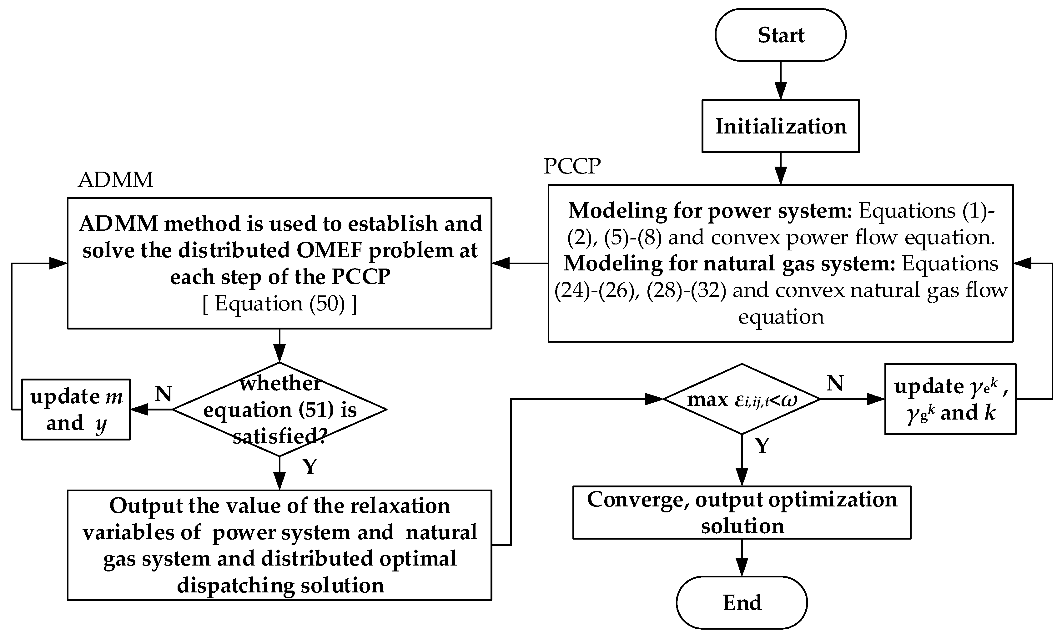
3.2. Decentralized Algorithm

The ADMM algorithm uses the ideas of dual decomposition and decoupling. It has the advantages of fast convergence and strong robustness. It is suitable for solving decentralized optimization problems, and the convex programming problem can be guaranteed to converge to the optimal solution through the ADMM algorithm.

Through the PCCP method, the power system and natural gas system have established corresponding convex models. In a decentralized framework, in order to ensure the convexity of the model, the ADMM algorithm is used to solve the decentralized OMEF problem at each iteration of PCCP.

First, according to the augmented Lagrange Equation, the coupling constraint (48) is relaxed into the objective function F, and the augmented Lagrange Equation is established as follows:

$$L(x^{\mathrm{e}},x^{\mathrm{g}},y)=F+y^T(x^{\mathrm{e}}-x^{\mathrm{g}})+\frac{\rho }{2}\left|\right|x^{\mathrm{e}}-x^{\mathrm{g}}|{|}_2^2$$

(49)

where y is the Lagrange multiplier; ρ is the step size, which is constant.

Then, this problem is transformed into two independent sub-optimization problems according to the ADMM method. Its iterative format is as follows:

$$\begin{array}{l}{Z}^{\mathrm{e},m+1}=\arg \min [F^{\mathrm{e}}+\mathsf{\Delta }\mathrm{e}+{(y^m)}^T(x^{\mathrm{e}}-x^{\mathrm{g},m})+\frac{\rho }{2}||x^{\mathrm{e}}-x^{\mathrm{g},m}|{|}^2]\\ Z^{\mathrm{g},m+1}=\arg \min [F^{\mathrm{g}}+\mathsf{\Delta }\mathrm{g}+{(y^m)}^T(x^{\mathrm{e},m+1}-x^{\mathrm{g}})+\frac{\rho }{2}||x^{\mathrm{e},m+1}-x^{\mathrm{g}}|{|}^2]\\ y^{m+1}=y^m+\rho (x^{\mathrm{e},m+1}-x^{\mathrm{g},m+1})\end{array}$$

(50)

where $Z^{\mathrm{e},m+1}$ and $Z^{\mathrm{g},m+1}$ are the iterative formats for power system optimization and natural gas system optimization problems; $F^{\mathrm{e}}$ is the objective function of power system optimization, including the cost of generating electricity from coal-fired units and penalty cost of wind power curtailment; $F^{\mathrm{g}}$ is the objective function of natural gas system optimization, including the cost of generating electricity from gas turbines and the cost of gas sources; $y^{m+1}$ is the iterative format of Lagrange multiplier; m is the number of iterations.

The convergence criteria for decentralized optimization are as follows:

$$\begin{array}{l}{r}^{m+1}=\left|\right|x^{\mathrm{e},m+1}-x^{\mathrm{g},m+1}\left|\right|\le \tau \\ s^{\mathrm{e},m+1}=\left|\right|x^{\mathrm{e},m+1}-x^{\mathrm{e},m}\left|\right|\le \tau \\ s^{\mathrm{g},m+1}=\left|\right|x^{\mathrm{g},m+1}-x^{\mathrm{g},m}\left|\right|\le \tau \end{array}$$

(51)

where $r^{m+1}$ is the original residual, which reflects the infeasibleness of the decentralized model; $s^{\mathrm{e},m+1}$ and $s^{\mathrm{g},m+1}$ are the dual residuals of the power system and the natural gas system, reflecting whether the iterative calculations have converged to the optimal solution; τ is the convergence accuracy.

The decentralized solution can be described as: The power system calculates the optimal energy flow value according to the iterative format $Z^{\mathrm{e},m+1}$, and passes the value of the boundary variable $x^{\mathrm{e},m+1}$ to the natural gas system. The natural gas system calculates the optimal energy flow value according to the iterative format $Z^{\mathrm{g},m+1}$, and passes the value of the boundary variable $x^{\mathrm{g},m+1}$ to the power system for the next iterative operation. During the system optimization process, the network topology, operating conditions, and calculation optimization processes of the power system and natural gas system are independent. The power and natural gas system make global adjustments by exchanging a small amount of boundary information to obtain a global optimal solution.

3.3. Flowchart of Decentralized OMEF Optimization Algorithm

The algorithm proposed in this paper first transforms the non-convex OMEF problem into a convex programming problem through PCCP, and then, performs a decentralized solution at each iteration of PCCP according to ADMM. The algorithm flowchart is shown in Figure 3.

The detailed solution steps of the algorithm are as follows:

Step 1: System partition. According to the node tearing method, the IEGS is divided into two regions: power system and natural gas system.

Step 2: Initialization. Set PCCP algorithm parameters and ADMM algorithm parameters, and use ADMM to solve the OMEF problem modeled with QC relaxed power flow model and the natural gas system model that ignores Equation (27) to obtain the initial value of the iteration in the PCCP process.

Step 3: Power system and natural gas system establish corresponding convex models according to PCCP method.

Step 4: According to the model obtained in step 3, the ADMM method is used to establish and solve the decentralized OMEF problem at each iteration of the PCCP. Determine whether the ADMM convergence criterion is satisfied, that is, whether Equation (51) is satisfied. If it is satisfied, the optimization result is output, and the process proceeds to step 5; otherwise, update the number of iterations m and the Lagrange multiplier y for the next optimization iteration.

Step 5: According to the partial output of step 4, that is, the value of the relaxation variables of the power system and the natural gas system determines whether all meet the PCCP convergence conditions (max ${\epsilon }_{i,ij,t}<\omega$). If both systems meet the convergence conditions, output of the optimization results; otherwise, update the penalty coefficients ${\gamma }_{\mathrm{e}}^k$ and ${\gamma }_{\mathrm{g}}^k$, the number of iterations k, and skip to step 3 to continue the optimization. To speed up the convergence, the value obtained at the kth iteration is set as the initial iteration value of k+1th iteration of PCCP and ADMM.

Step 6: Output calculation results.

4. Case Studies

In order to verify the accuracy of the algorithm proposed in this paper, case studies are carried out on a testing IEGS combined with an IEEE 39-bus power system and a Belgian 20-bus natural gas system. The topology of testing IEGS is shown in Appendix A, Figure A1. The proposed model and algorithm are implemented with GAMS and Matlab2019a, where GAMS is to as an optimization solver to solve the problem, and Matlab2019a is to call and analyze the calculation results from GAMS.

4.1. Simulation Model Description

In this simulation model, there are five coal-fired units, three gas turbines, and two wind turbines in the IEEE 39-bus power system. There are two gas sources, four gas storage tanks, and three natural gas compressors in the Belgian 20-bus natural gas system. The gas turbines (GT₁, GT₂, GT₃) are connected to gas nodes 4, 10, 12 respectively. The input terminals of P2Gs are connected to the electricity nodes 33, 34, respectively, and the corresponding output terminals are connected to the gas nodes 13, 14. The initial total line pack is 5.86 × 10⁶ m³. The cost factor of wind power curtailment is set as d_i = 50$/MW∙h. Other main parameters of the simulation model are shown in the Appendix A

Table A1. Parameters of units.

Units	Cost Factor			Maximum Output
				Active Output (MW)	Reactive Output (MVar)
	a2	a1	a0
GM1	0.700	26.987	0	646	300
GM2	0.682	21.978	0	725	300
GM3	0.425	25.00	0	687	300
GM4	0.458	26.098	0	865	300
GM5	0.890	26.176	0	1100	300
	bi
GT1	0.25			1040	400
GT2	0.25			580	240
GT3	0.25			564	250
	di
WT1	50			652	250
WT2	50			508	167

,

Table A2. Parameters of gas sources.

Units	Cost Factor ci($/m3)	Minimum Output (m3/s)	Maximum Output (m3/s)
S1	0.25	10.3	105.5
S2	0.25	12.0	104.2

,

Table A3. Parameters of P2Gs.

Units	${\mathit{\alpha }}_{\mathbf{P}2\mathbf{G},\mathit{i}}$	${\mathit{C}}_{\mathbf{g},\mathit{i}}$
P2G1	0.6	39
P2G2	0.6	39

and

Table A4. Parameters of GTs.

Units	z2,i	z1,i	z0,i
GT1	0.0769	5.9769	0
GT2	0.0450	5.4692	0
GT2	0.0601	5.5242	0

. The curve of electric load and gas load is shown in Figure 4. This paper takes one day with 24 h as a dispatch cycle.

4.2. Analysis of the Algorithm

In order to verify the accuracy of the decentralized framework and algorithm for the OMEF problem proposed in this paper, the algorithm solving process and optimization results are analyzed in detail. The key parameters of the algorithm in this paper are shown in

Table 1. The parameters of the algorithm.

Algorithm		Parameters
PCCP	power system	${\gamma }_{\mathrm{e}}^0$	${\gamma }_{\mathrm{e},\max }$	${\mu }_{\mathrm{e}}$	${\omega }_{\mathrm{e}}$
		10	1000	2	0.1
	natural gas system	${\gamma }_{\mathrm{g}}^0$	${\gamma }_{\mathrm{g},\max }$	${\mu }_{\mathrm{g}}$	${\omega }_{\mathrm{g}}$
		0.1	100	2	0.01
ADMM		ρ		τ
		1000		0.01

.

In order to verify the accuracy and effectiveness of the decentralized algorithm proposed in this paper, the decentralized optimization results are compared with the centralized algorithm.

As shown in

Table 2. Performance of PCCP-ADMM algorithm.

Algorithm		Objective($)	Iteration	Time(s)
centralized optimization	NLP	5.3164 × 106	83	4.19
	PCCP	4.9680 × 106	5	45.26
decentralized optimization	PCCP-ADMM	4.9881 × 106	22	68.18

, the NLP algorithm is to solve the OMEF problem of IEGS without processing non-convex equations. Meanwhile, the PCCP algorithm is to use the PCCP method proposed in this paper to model for the power system and the natural gas system and solve it centrally. Comparing the two results, although NLP can directly use the IPOPT solver to solve the OMEF problem, the results obtained are not optimal solutions, and the non-convex nature makes the decentralized algorithm unable to converge or obtain ideal results. The PCCP algorithm used to solve the OMEF problem can converge to an optimal solution. PCCP-ADMM algorithm is the decentralized algorithm proposed in this paper. Compared with the PCCP centralized algorithm, the results obtained by the decentralized algorithm are similar to the centralized algorithm, which verifies the feasibility of the decentralized algorithm. The difference between the two results is 0.4%, which is acceptable. For optimization time, the decentralized algorithm takes more time than the centralized algorithm. However, the decentralized algorithm only needs to exchange a small amount of boundary information in each area to coordinate the global optimal scheduling, which guarantees the privacy of the information in each area.

The iterative process of PCCP-ADMM algorithm is shown in Figure 5. It can be seen from (a) that the optimization process performed 7 PCCP iterations and 22 ADMM iterations. As shown in (b), at the boundary of each iteration of PCCP, the ADMM residual will basically increase, because the algorithm’s solution mechanism is that the ADMM algorithm is performed at each iteration of PCCP, but the overall trend is declining. In addition, in the second iteration of PCCP and later, the number of ADMM iterations is small. The reason is that the energy flow results obtained by the PCCP-ADMM in these steps are close to the optimal solution, and the ADMM algorithm in k+1th iteration of PCCP uses the Lagrange multiplier result in kth iteration as the initial iteration value. Therefore, the proposed algorithm can not only guarantee convergence to the optimal solution, but also speed up the convergence speed.

4.3. Analysis of Optimization Results

The PCCP-ADMM algorithm proposed in this paper is used to solve and the OMEF problem. In order to analyze the impact of the dynamic characteristics of the natural gas system on the optimal scheduling of the system, this paper analyzes the following two cases:

(1)

Case 1: Regardless of the dynamic characteristics of the natural gas system (i.e., removing the Equations (24)–(26)), the objective is to optimize the cost of energy supply.

(2)

Case 2: Considering the dynamic characteristics of the natural gas system, the objective is to optimize the cost of energy supply.

This paper uses PCCP-ADMM algorithm to optimize two cases and analyzes the results to research the impact of the line pack on the optimal operation of the system, as shown in Figure 6 and Figure 7.

According to the optimization results, during the period of 1–6 h, the system’s electric and gas loads are in the trough period. Compared with Case 1, Case 2 has more gas sources output, and part of the gas is stored in the natural gas pipeline. As shown in Figure 6, the value of the total line pack rises. During the period of 8–12 h, the system load is at its peak. The load in the natural gas system in Case 1 is mainly satisfied by the output of the gas sources; in Case 2, during this period, there is a certain amount of the line pack to release, and the output of the gas sources is less. Therefore, considering the dynamic characteristics of natural gas systems, IEGS can buffer the gas inflow and gas outflow. The gas network has a certain energy storage capacity, which can effectively buffer load fluctuations. It improves the flexibility of the system operation while ensuring the quality of energy supply.

The cost of energy supply in each case is shown in

Table 3. Comparison of costs in different cases.

Case	Objective($)	Reduction (%)
1	5.0267 × 106	0.77
2	4.9881 × 106

. In Case 2, the cost is reduced due to the release of the line pack during the peak load period and used for system scheduling, with a reduction of 0.77%.

This paper focuses on Case 2. The output of some devices in the IEGS is shown in Figure 8.

For the power system, according to Figure 8b,d, it can be obtained that during the periods of 1–6 h and 22–24 h (load trough periods), the wind power output is relatively high. In order to absorb wind power, the excess power is injected into the natural gas system through P2Gs. In this period, P2Gs are basically close to full load operation. As shown in Figure 8a, during the period of 8–21 h, because the generating cost of coal-fired units is generally lower than that of gas turbines, coal-fired units are basically close to full power output; meanwhile the output of gas turbines is relatively flat, which is mainly output at peak loads.

For the natural gas system, as shown in the Figure 8c, it can be found that during the period of 2–6 h, the excess wind power is injected into the gas network through P2Gs and a part of it is stored in the gas storage tanks, and the gas inflow of the gas storage tanks is large. During the period of 8–12 h, due to the increase of system load, the gas storage tanks increase the gas outflow to meet the load demand.

5. Conclusions

Considering the dynamic characteristics of the natural gas system, the privacy of each system’s information, and the non-convexity of the OMEF model, this paper proposes a PCCP-ADMM decentralized algorithm to solve the OMEF problem. The simulation analysis of the testing IEGS proves the effectiveness of the algorithm and reaches the following conclusions:

(1)

For the non-convex OMEF model, this paper introduces the PCCP method to transform the non-convex OMEF problem into a convex programming problem, and proves the feasibility of the method from theoretical and simulation results.

(2)

This article analyzes the impact of the line pack on system performance. The calculation results show that considering the dynamic characteristics of the natural gas system can improve the flexibility and economy of the system.

(3)

Considering the privacy of the information of each subsystem in IEGS, this paper proposes a decentralized optimization algorithm for the OMEF problem based on PCCP-ADMM. In decentralized optimization, each system only needs to exchange a small amount of information to perform global coordination and optimization.

References

1. Wang, C.; Lv, C.; Li, P.; Song, G.; Li, S.; Xu, X.; Wu, J. Modeling and optimal operation of community integrated energy systems: A case study from China. Appl. Energy 2018, 230, 1242–1254. [Google Scholar] [CrossRef]
2. Behar, O. A novel hybrid solar preheating gas turbine. Energy Convers. Manag. 2018, 158, 120–132. [Google Scholar] [CrossRef]
3. Kirchbacher, F.; Biegger, P.; Miltner, M.; Lehner, M.; Harasek, M. A new methanation and membrane based power-to-gas process for the direct integration of raw biogas—Feasability and comparison. Energy 2017, 146, 34–46. [Google Scholar] [CrossRef]
4. Zhou, K.; Yang, S.; Shao, Z. Energy Internet: The business perspective. Appl. Energy 2016, 178, 212–222. [Google Scholar] [CrossRef]
5. Nastasi, B.; Basso, G.L. Power-to-Gas integration in the Transition towards Future Urban Energy Systems. Int. J. Hydrogen Energy 2017, 42, 23933–23951. [Google Scholar] [CrossRef]
6. Liu, W.; Wen, F.; Xue, Y. Power-to-gas technology in energy systems: Current status and prospects of potential operation strategies. J. Mod. Power Syst. Clean Energy 2017, 5, 439–450. [Google Scholar] [CrossRef] [Green Version]
7. Shahidehpour, M.; Fu, Y.; Wiedman, T. Impact of Natural Gas Infrastructure on Electric Power Systems. Proc. IEEE 2005, 93, 1042–1056. [Google Scholar] [CrossRef]
8. Urbina, M.; Li, Z. A combined model for analyzing the interdependency of electrical and gas systems. In Proceedings of the 2007 39th North American Power Symposium, Las Cruces, NM, USA, 30 September–2 October 2007; pp. 468–472. [Google Scholar]
9. Martinez-Mares, A.; Fuerte-Esquivel, C.R. A Unified Gas and Power Flow Analysis in Natural Gas and Electricity Coupled Networks. IEEE Trans. Power Syst. 2012, 27, 2156–2166. [Google Scholar] [CrossRef]
10. Correa-Posada, C.M.; Sanchez-Martin, P. Integrated Power and Natural Gas Model for Energy Adequacy in Short-Term Operation. IEEE Trans. Power Syst. 2015, 30, 3347–3355. [Google Scholar] [CrossRef]
11. Shahidehpour, M.; Liu, C.; Wang, J. Cordinated scheduling of electricity and natural gas infrastructures with a transient model for natural gas flow. Chaos 2011, 21, 025102. [Google Scholar]
12. Fang, J.; Zeng, Q.; Ai, X.; Chen, Z.; Wen, J. Dynamic Optimal Energy Flow in the Integrated Natural Gas and Electrical Power Systems. IEEE Trans. Sustain. Energy 2017, 9, 188–198. [Google Scholar] [CrossRef]
13. Chen, X.; Wang, C.; Wu, Q.; Dong, X.; Yang, M.; He, S.; Liang, J. Optimal operation of integrated energy system considering dynamic heat-gas characteristics and uncertain wind power. Energy 2020, 198, 117270. [Google Scholar] [CrossRef]
14. Wang, S.; Wang, S.; Chen, H.; Gu, Q. Multi-energy load forecasting for regional integrated energy systems considering temporal dynamic and coupling characteristics. Energy 2020, 195, 116964. [Google Scholar] [CrossRef]
15. Bao, Z.; Ye, Y.; Wu, L. Multi-timescale coordinated schedule of interdependent electricity-natural gas systems considering electricity grid steady-state and gas network dynamics. Int. J. Electr. Power Energy Syst. 2020, 118, 105763. [Google Scholar] [CrossRef]
16. Qu, K.; Zheng, B.; Yu, T.; Li, H. Convex decoupled-synergetic strategies for robust multi-objective power and gas flow considering power to gas. Energy 2019, 168, 753–771. [Google Scholar] [CrossRef]
17. He, Y.; Yan, M.; Shahidehpour, M.; Li, Z.; Guo, C.; Wu, L.; Shao, C. Decentralized Optimization of Multi-Area Electricity-Natural Gas Flows Based on Cone Reformulation. IEEE Trans. Power Syst. 2018, 33, 4531–4542. [Google Scholar] [CrossRef]
18. Qu, K.; Shi, S.; Yu, T.; Wang, W. A convex decentralized optimization for environmental-economic power and gas system considering diversified emission control. Appl. Energy 2019, 240, 630–645. [Google Scholar] [CrossRef]
19. Stott, B.; Jardim, J.; Alsac, O. DC Power Flow Revisited. IEEE Trans. Power Syst. 2009, 24, 1290–1300. [Google Scholar] [CrossRef]
20. Jabr, R.A. Radial Distribution Load Flow Using Conic Programming. IEEE Trans. Power Syst. 2006, 21, 1458–1459. [Google Scholar] [CrossRef]
21. Correa-Posada, C.M.; Sanchez-Martin, P. Security-Constrained Optimal Power and Natural-Gas Flow. IEEE Trans. Power Syst. 2014, 29, 1780–1787. [Google Scholar] [CrossRef]
22. Bischi, A.; Taccari, L.; Martelli, E.; Amaldi, E.; Manzolini, G.; Silva, P.; Campanari, S.; Macchi, E. A detailed MILP optimization model for combined cooling, heat and power system operation planning. Energy 2014, 74, 12–26. [Google Scholar] [CrossRef]
23. Wang, C.; Wei, W.; Wang, J.; Bai, L.; Liang, Y.; Bi, T. Convex Optimization Based Distributed Optimal Gas-Power Flow Calculation. IEEE Trans. Sustain. Energy 2018, 9, 1145–1156. [Google Scholar] [CrossRef]
24. Wang, C.; Wei, W.; Wang, J.; Wu, L.; Liang, Y. Equilibrium of Interdependent Gas and Electricity Markets with Marginal Price Based Bilateral Energy Trading. IEEE Trans. Power Syst. 2018, 33, 4854–4867. [Google Scholar] [CrossRef]
25. Tian, Z.; Wu, W. Recover Feasible Solutions for SOCP Relaxation of Optimal Power Flow Problems in Mesh Networks. IET Gener. Transm. Distrib. 2019, 13, 1078–1087. [Google Scholar] [CrossRef] [Green Version]
26. Low, S.H. Convex Relaxation of Optimal Power Flow—Part I: Formulations and Equivalence. IEEE Trans. Control Netw. Syst. 2014, 1, 15–27. [Google Scholar] [CrossRef] [Green Version]
27. Van Hertem, D.; Verboomen, J.; Purchala, K.; Belmans, R.; Kling, W. Usefulness of DC power flow for active power flow analysis with flow controlling devices. In Proceedings of the 8th IEE International Conference on AC and DC Power Transmission, London, UK, 28–31 March 2006; pp. 58–62. [Google Scholar]
28. Coffrin, C.J.; Hijazi, H.L.; Van Hentenryck, P. The QC Relaxation: A Theoretical and Computational Study on Optimal Power Flow. IEEE Trans. Power Syst. 2016, 31, 3008–3018. [Google Scholar] [CrossRef]
Figure 1. Framework of IEGS.
Applsci 10 03348 g001
Figure 2. Decentralized framework.
Applsci 10 03348 g002
Figure 3. Algorithm flowchart.
Applsci 10 03348 g003
Figure 4. The curve of electric load and gas load.
Applsci 10 03348 g004
Figure 5. Iterative process of PCCP-ADMM: (a) The number of iterations of ADMM in each iteration of PCCP; (b) The convergence process of residuals in the overall iteration.
Applsci 10 03348 g005
Figure 6. Change of the total line pack.
Applsci 10 03348 g006
Figure 7. Output of gas sources in different cases.
Applsci 10 03348 g007
Figure 8. Output of some devices in Case 2: (a) Output of some devices in the power system; (b) Output of wind turbines; (c) Output of some devices in the natural gas system; (d) Output and input of P2Gs.
Applsci 10 03348 g008