Advanced Methods for Point Cloud Processing and Simplification

Abstract

Nowadays, mobile robot exploration needs a rangefinder to obtain a large number of measurement points to achieve a detailed and precise description of a surrounding area and objects, which is called the point cloud. However, a single point cloud scan does not cover the whole area, so multiple point cloud scans must be acquired and compared together to find the right matching between them in a process called registration method. This method requires further processing and places high demands on memory consumption, especially for small embedded devices in mobile robots. This paper describes a novel method to reduce the burden of processing for multiple point cloud scans. We introduce our approach to preprocess an input point cloud in order to detect planar surfaces, simplify space description, fill gaps in point clouds, and get important space features. All of these processes are achieved by applying advanced image processing methods in combination with the quantization of physical space points. The results show the reliability of our approach to detect close parallel walls with suitable parameter settings. More importantly, planar surface detection shows a 99% decrease in necessary descriptive points almost in all cases. This proposed approach is verified on the real indoor point clouds.

1. Introduction

The main remote sensing task is to obtain a large number of measurement points to achieve a detailed and precise description of a surrounding area and objects in a scanned space. The inseparable part constitutes their processing to obtain desired input data for the purpose of the application which the scanning was used for. There are many different applications where the processing of remote sensing is important; see the following subsections for how to deal and process point clouds.

The main issue of our research is point cloud processing and simplification with the focus on the detection, statistical description, vectorization, and visualization of basic space features. This will allow the decreased memory consumption of physical data storage. For example, individual points of a planar surface composed of a thousand points are not so important for the subsequent processing. We rather look for vertices of the analyzed planar surface. Our contribution in point cloud processing is to show a different alternative way of processing. The main advantages of our approach lie in the combination of the physical space points quantization with image processing methods. This connection allows: obtaining important space features such as the area, perimeter and volume; the space and statistical descriptions of planar surfaces, including the descriptive point amount decreasing by the vectorization of vertices; the correction and recovery of missing space data; and a planar surface presented as the image allows the alternative way of the physical points storage, including its visualization. It also serves to other researchers as the extension to the used methods presented in the following subsection. Moreover, the presented approach is usable not only for point clouds but also as the general processing and analysis of different levels for any 3D data.

This paper is focused on the presentation of several new methods for point cloud processing such as the outlier points removal, estimation of the initial point cloud rotation, point cloud data correction and recovery, and the vertices detection of a planar surface. In the Introduction section is a survey about different point cloud processing methods for basic object detection and segmentation, the planar surface and space features estimation, and their typical application. The paper further includes the description of our developed point cloud processing pipeline and the presentation of the new methods in detail to give a comprehensive overview of our developed approach, including verification on real space data. In the results part, the processing of the complex point cloud with several rooms is presented. The results and algorithms are evaluated also in terms of precision against the physical space dimensions and comparison with the convex hull results. The recommendations for this processing approach are stated.

1.1. Related Works

A wide survey of 3D surface reconstruction methods is provided in reference [1]. The authors accurately and in a well-arranged way evaluated the state-of-the-art methods with their advantages and disadvantages. The survey includes a table of all methods, where the main features and the possibility of use are summarized.

Valuable work is presented by the authors in reference [2]. The paper deals with the automatic reconstruction of the fully volumetric 3D building models from oriented point clouds. The proposed method can process the large complex real-world point clouds from the unfiltered form into the separated room model, including suppressing of undesired objects inside a room. Several methods for 3D modelling an indoor environment relying explicitly on the prior knowledge of scanner positions are in reference [3]. In many software products provided by a manufacturer of scanners, the scanning position is irretrievably lost. Therefore, the authors propose a method for the reconstruction of the original position of the scanners. The presented method can determine these positions also under very unfavorable conditions. The next research focuses on the estimation of surface geometries directly from a point cloud as in reference [4]. It introduces the 3D surface estimation method of the household objects inside the area. The authors developed a Global Principal Curvature Shape Descriptor (GPCSD) for the categorization of objects into groups. The main purpose is to improve the manipulation planning for a robotic hand.

Researchers in reference [5] introduced a point cloud segmentation method for urban environment data. Their method is based on the robust normal estimation by the construction of an octree-based hierarchical representation for input data. The achieved results prove the concept of usability for the urban environment point clouds even if there is space for improving the detection of some regular objects with curved surfaces. The octree-based approach, with a combination of PCA analysis, is presented in reference [6]. Results are compared with other detection algorithms such as a 3D Kernel-based Hough Transform (3D-KHT) or the classical Random Sample Consensus (RANSAC). This method provides accurate results, robustness to noise, and the possibility to detect planes with small angle variations. The similar research in reference [7] focuses on the plane segmentation of building point clouds. The proposed Density-Based Spatial Clustering of Applications with Noise (DBSCAN) method also respects the curvatures to provide the final fine segmentation. The DBSCAN clustering for surface segmentation is used also in reference [8]. A part, in which the results are presented, shows the desired surface segmentation, but only in a simple point cloud, which is not a real-world case. The surfaces can be extracted also from the RGBD images (see reference [9]). The proposed split and merge approach produces interesting visual results. The planes are detected from depth images by the Depth-driven Plane Detection (DPD) algorithm based on a region grooving (see reference [10]). The Hough transformation (HT) approach called D-KHT can be used for a plane segmentation from these images, as it is shown in reference [11]. Due to the properties of the HT, this method can detect the planes with discontinuities. The ground plane detection using the depth maps captured by a stereo camera is presented in reference [12]. The camera is moving, and the system deals with the elimination of their roll angle for the correct plane segmentation.

The growing topical issue of deep learning in recent years is used for point cloud segmentation. One case of use is indoor boundary estimation (see reference [13]). The described method relies on the depth estimation and wall segmentation to generate the exterior point cloud. The deep supervised clustering helps to fit the wall planes to obtain the resulting boundary map. In a different research work, the deep learning method called PCPNet is used to estimate local 3D shape properties in point clouds (see reference [14]). The main purpose is to classify the objects and shapes or do semantic labeling. The presented results show good estimation ability for the normals and the curvatures, even in the noisy point clouds. The deep learning approach is likewise used on automatic building detection and segmentation from the aerial images or the point clouds (see reference [15]). The main focus lies in improving and preparing high-quality training data, which allows better segmentation of the detected objects. The presented results show the high detection accuracy (higher than 90%) with the RGB-lidar and the fused RGB-lidar data of the urban scenes. The next research (shown in reference [16]) presents the new topology-based global 3D point cloud descriptor called Signature of Topologically Persistent Points (STPP). The topological grouping improves the detection robustness and increases the resistance against a noise. The complementary information also improves deep learning performance. The different topological method TopoLAB described in reference [17], that no longer uses neural networks, focuses on a pipeline to recover the broken topology of planar primitives during the reconstruction of complex building models. Due to the scanning difficulties and a variable point cloud density, some parts of a model can be missing. The proposed method allows the recovery of these parts, including to visualize the different levels of the details.

With respect to the safety and health of the persons, the laser scanning plays an important role in exploring abandoned or dangerous places like various mines (see reference [18]). Similar to this use is the scanning of rock masses (see reference [19]). The proposed method for the planar surface extraction is able to deal with rough and complex surfaces.

For the Mobile Laser Scanning (MLS), the new method Planes detection and Segmentation is proposed based on the Planarity values of Scan profile groups (PSPS) (see reference [20]). The presented results prove the quality of this method in comparison with other state-of-the-art algorithms for these types of spare point clouds, for example, the segmented planar surfaces stand out by their compactness.

The 3D point cloud processing is important not only to get physical shapes, but also it can be used to quantitatively characterize the height, width, and volume of shrub plants. Authors in reference [21] analyze point clouds of different blueberry genotype groups to improve the mechanical harvesting process. For comparison of different shrubs, the correlation is used. In the study described in reference [22], the researchers focus on the filtering method of leaves based on the manifold distance and the normal estimation. The scanned leaves contain the outliers and the noise. The precise estimation of the shape and area of a leaf is important to obtain the tree growth index. Moreover, also the ground plane segmentation plays an important role in the analysis of asparagus harvesting (see reference [23]). The asparagus stems are scanned by a modern time-of-flight camera, which ranks as the fastest scanning device. The proposed Hyun method outperformed the classical RANSAC method in a scene with high clutter. Similar to the previous works is a parametrization of the forest stand described in reference [24]. The researchers propose to use, instead of leaf area index, other space characteristics such as the stand denseness, canopy density, crown porosity, and others. In the practical part, they discovered a high correlation index between each other. The geometric characterization of vines from 3D point clouds is important in the agronomy sector (see reference [25]). The convex hull method is used for calculating the volume of these plants. The recent research in reference [26] deals also with this method in the aim to find the shortest path in 2D complexes with non-positive curvatures. The convex hull method is often used for the determination of an area and perimeter in 2D shapes.

Point cloud processing, object detection and segmentation are widely used in various research areas for different purposes as is shown above. The right processing method choice helps with the extraction of desired information. Input data transformation into the different forms allows the easy obtaining of an unknown feature.

1.2. Our Point Cloud Processing Contribution

The first work of object detection, which we proposed, was the algorithm for point cloud unfolding into a single plane with height preservation, as in reference [27]. The presented method works correctly for rectangular rooms with four walls, a known scanner position, and walls not occupied by many objects. The aim of this work was to unfold all walls with objects into a single plane. The single plane representation allows the removal of walls close to zero and analyzing of the remaining objects. Finally, this method proved to be a dead-end for follow-up utilization. The unfolding of the objects placed on the corner splitting line caused their division into two parts. The global position of the object is also lost.

Many researchers are using depth images in their work (as shown in references [9,10,11,12,13]). The depth images contain the real physical sizes and distances which are possible to utilize further. We had a point cloud without depth information, so we decided to develop the algorithm for the depth map construction, which we described in reference [28]. The main advantage of this algorithm lies in the possibility to create a depth map from any point cloud with the arbitrary camera position and arbitrary camera orientation. The concept of space quantization has shown to be useful for further space data processing. Moreover, we can process these images by image processing methods and for example, transform depth pixels back into the point cloud by using the reverse process. The depth image includes space information about the structure and the quality of an analyzed surface. The depth image offers to detect surfaces or other objects (see references [9,10,11,12,13]). A depth camera covers only the area, which is seen by the camera itself. This is the main disadvantage for global object detection and segmentation. Some objects cover the other objects and areas present in a scene. For this reason, a depth image is not suitable for global space segmentation and description, but the space quantization into the image with a connection of image processing methods offers wide possibilities for basic object detection and detailed space description.

In the papers [29,30], we introduced a novel algorithm called the Level Connected Component Labeling (LCCL) for global 3D data analysis in terms of detecting global levels with high data concentration in selected space dimensions. A planar surface presence is indicated mainly by the high concentration of points in the particular dimension at the specific level. To find the high point concentration at the specific level is not sufficient for planar surface detection. Several planar surfaces can be present in one of the detected levels. Thus, we are using space quantization into an image for this purpose. This allows the use of classically connected labeling to separate individual planar surfaces. A planar surface is presented by the tool called Level Image ($L_I$), which is described in references [29,30,31,32]. For each $L_I$, its origin and rotation angle are known. The surface selected dimension is calculated as the average of the points on this surface. From the LCCL output, the statistical parameters, such as the mean value, variance, standard deviation, and data mode, are also known. These parameters describe the quality of the detected planar surface.

The connection of a $L_I$ with image processing methods allows expression of a planar surface area and perimeter [30] or interactive visualization [31], including color presentation when available. One of our last research works [32] deals with fine plane range estimation. In this paper, we will present the next methods for point cloud preprocessing and processing, which we did not publish yet, helping to decrease a point amount for the planar surface description, fill the gaps in the point clouds, and obtain other important space features.

2. Point Cloud Processing Approach

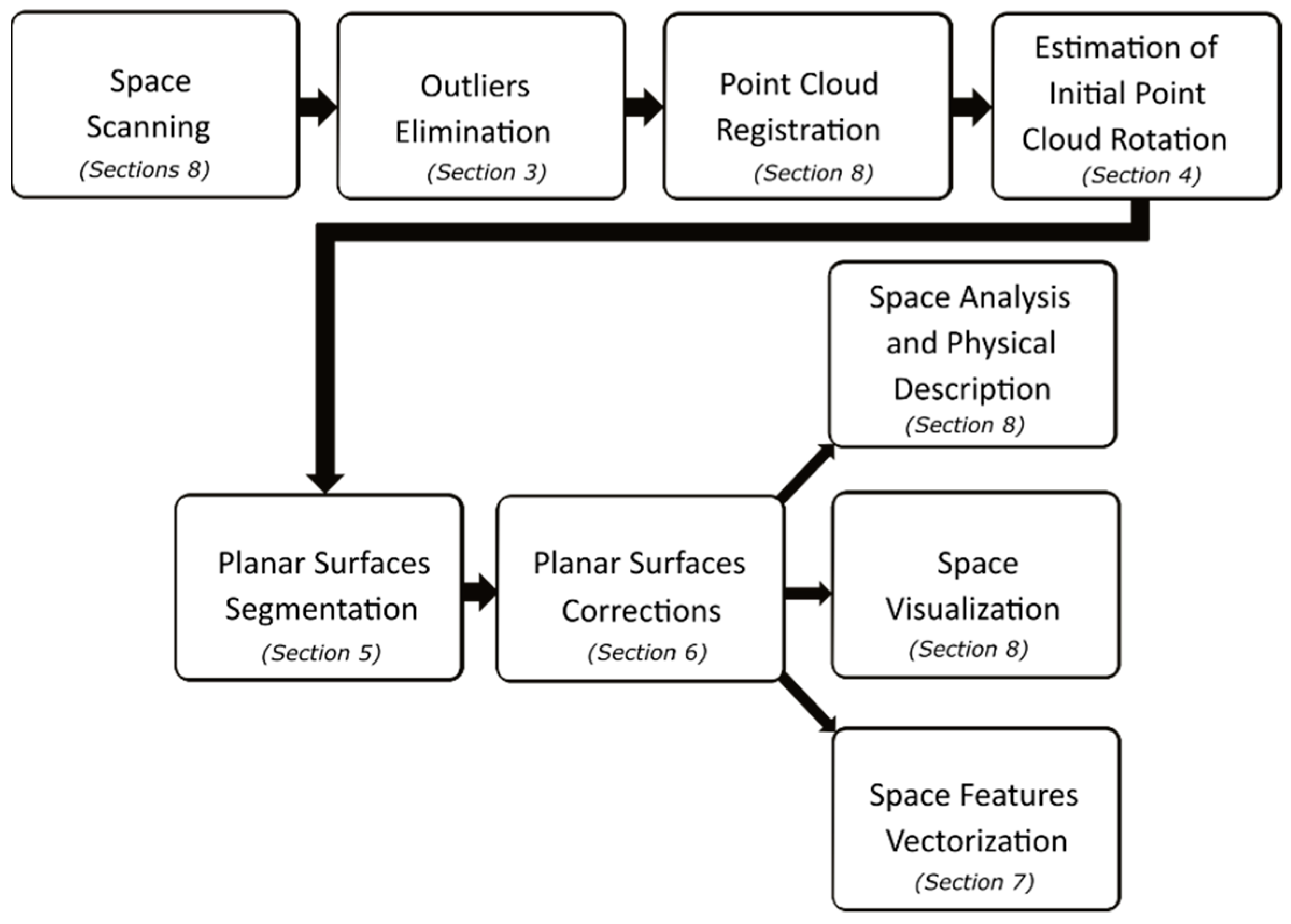
Following Figure 1 shows the processing diagram of a point cloud in the form of how it is introduced in this paper. Each block is marked by the section where a method is described or at least mentioned. This paper is mainly focused on four parts of our proposed processing approach, which we did not present before, concretely the outlier elimination; estimation of initial point cloud rotation; possible point cloud correction, such as fill gaps in detected planar surfaces; and vectorization of basic detected shapes for the purpose of decreasing the number of points.

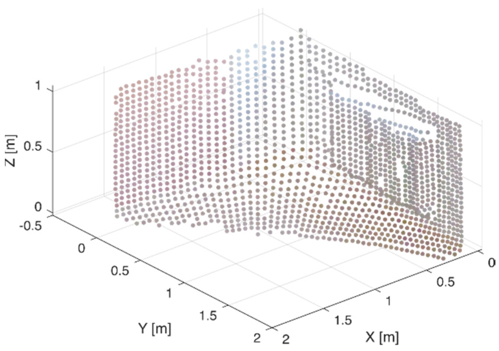
The aim of this paper is to present the methods on how to process point cloud data from a 3D scanner to achieve the desired segmentation, visualization and physical space description. The main contribution of our proposed approach is the connection of algorithms with image processing, which allows correction of scanned data; obtaining important space features easily; or even making color space visualization possible. Moreover, for planar surface detection, we can use any of the described methods from Section 1 to get segmented parts of a point cloud and apply the proposed approach in this paper for their further processing. The following sections describe the developed methods in detail. For their description, the point cloud model depicted in Figure 2 is used.

The point cloud is the real edge of a room with the radiator. This simple model nicely illustrates the environment with several planar surfaces of different sizes and origins in a space.

3. Outlier Points Elimination

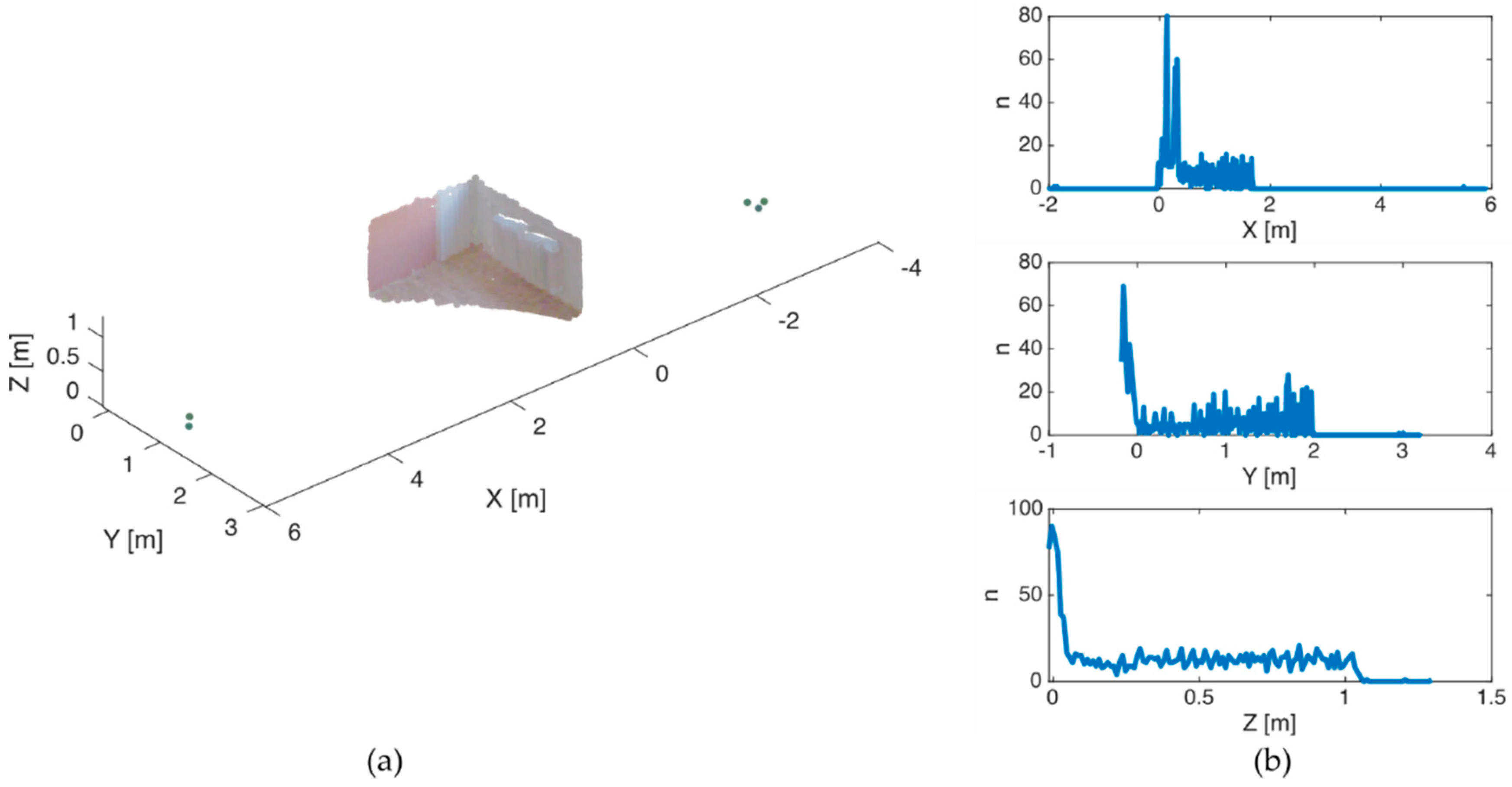
Due to the rangefinder measurement errors, a final point cloud may contain outlying points. These points have an unfavorable influence on the overall details during the point cloud visualization, but mainly they caused problems with point cloud registration. Figure 3a illustrates the visualization of the influence of several outlying points. To illustrate this issue, the five outlying points were added into the model in Figure 2. The problem is that only one outlying point will cause the same undesired visual look. The histograms of the measurement point concentrations of all coordinate axes are shown in Figure 3b.

Outlying points caused mainly problems in point cloud registration. Our presented processing pipeline in Figure 1 entails in more iteration steps of the algorithms. The method for far point elimination uses just these histograms and concentration of points in a specific level of coordinate axes. Histograms are marked as $h_X$, $h_Y$, and $h_Z$. The proposed method uses the user defined threshold $h_T$ defining the minimal concentration of points. The histogram of the axis is marked as $h_d$, and this is used for the definition of the general equation, where $d$ denotes the coordinate axis. Then, the histogram is described by the following equation:

$$h_d(n)=\#X\left(v_d(n,1):v_d(n,2),d\right),$$

(1)

where $X$ is the input point cloud, the symbol $\#$ denotes the number of selected points by the individual density ranges of the histogram $v_d$. The value $n\in \left[1,2,\dots ,N_d\right]$ is the actual range index of the total count of the values defined from the equation.

$$N_d=\left(\max \left(X(\forall ,d)\right)-\min \left(X(\forall ,d)\right)\right)\cdot 1e^3.$$

(2)

Equation (2) is multiplied by the constant $1e^3$ expressing the millimeter resolution, denoted as histogram step $h_{St}$. The $v_d$ values are step ranges of the histogram obtained from the range of the analyzed axis $h_{Rd}$, defined as:

$$h_{Rd}=\left[\min (X(\forall ,d)),\max (X(\forall ,d))\right];$$

(3)

total count of values $N_d$ from Equation (2); and its step $h_{St}$. Values of $v_d$ consist of $N_d$ rows and two columns marked as 1 and 2 in Equation (1) define starts and ends of the individual ranges of the histogram. The threshold value $h_T$ for the elimination outliers is set by the user. It is applied on both sides of the histogram $h_d$ as the first value higher than the threshold.

$$h_d(n)\ge h_T.$$

(4)

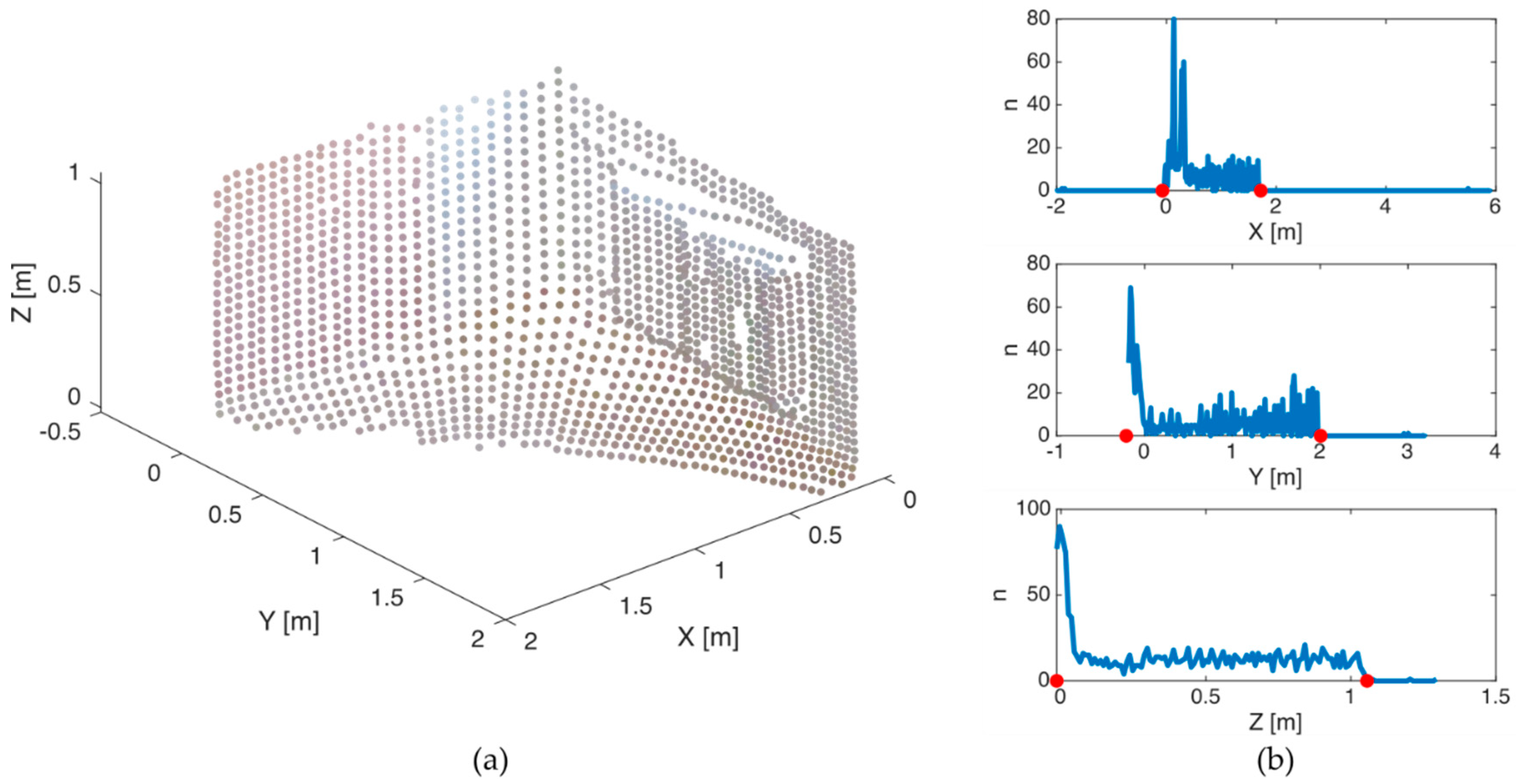
Following Figure 4 gives the point cloud from Figure 3 with removed outliers and threshold value $h_T=2$. The new narrower range of the histograms is marked by two red dots in Figure 4b.

The final point clouds are suitable for the registration process and further processing. The initial point cloud rotation is important for some object segmentation algorithms, like our algorithm for surface detection. The known initial rotation substantially speeds-up the detection process. Next, Section 4 deals with the initial rotation estimation of a point cloud.

4. Correction of Initial Point Cloud Rotation

A space 3D scanner is usually placed into a scanned space on several positions sequentially. Each scanner positioning can be influenced by the wrong heading of the scanner even in a few angle degrees. This fact is negligible for the registration process but, for example, when the first point cloud is influenced by this error, the composed final point cloud is rotated in the same way. The knowledge of an initial point cloud rotation angle is necessary for the best results and the speed assurance of our proposed methods. We can also rotate by the point cloud in a prescribed range of angles (see reference [29]) and find the best match of points in the detected planar surfaces, but this is time-consuming and inefficient. We developed the following approach for the purpose of finding the initial rotation angle of a point cloud.

A density histogram of the points in the individual axes is also possible to use for the correction of a point cloud rotation. This correction can be likewise applied before the registration process on individual point clouds. It improves the registration success probability. The known orientation angle of the point cloud significantly improves the processing time in our proposed methods for point cloud processing.

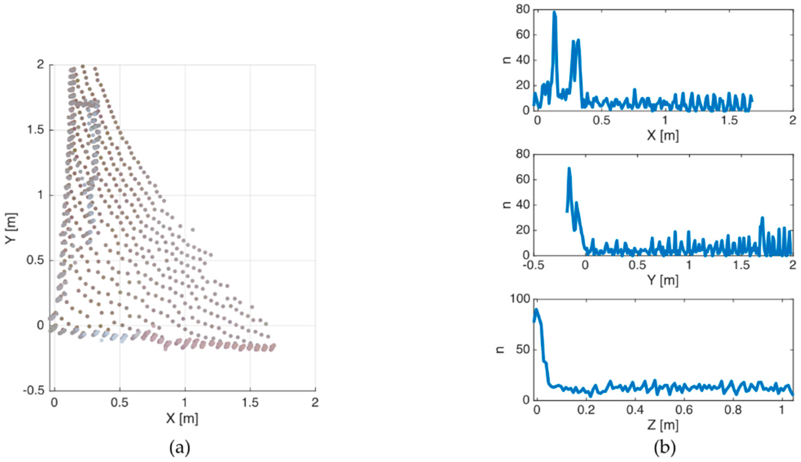
The main assumption for its success lies in the presence of flat surfaces in the input point cloud, which is true in most cases of indoor space. The point cloud with correct orientation in the X and Y axes is shown in Figure 5a. Its bottom planar surface is parallel to the zero level in the Z-axis. The unknown parameter is the rotation in the Z-axis. Figure 5b gives constructed histograms of all coordinate axes with a resolution of 1 mm.

The developed method for the estimation of the initial rotation is able to determine the rotation angle of one coordinate axis from the two others. The one main maximum is noticeable in the histogram of the Z-axis, as is shown in Figure 5b. Its position marks the floor of the edge. In the case of the X and Y axes, the maxima of histograms represent the walls of the model and the radiator. The proposed method analyzes these maxima in the prescribed range of the rotation angles to estimate the correction angle of the initial rotation.

In the following example, shown in Figure 6, the rotation estimation of the Z-axis from the X and Y axes is shown. The flat surfaces in the analyzed point cloud may occur in different levels. It is necessary to analyze all local maxima from this reason, and not only the biggest. Their values may also vary depending on a concentration of points. To get these maxima from a histogram, we use the modified algorithm for the connected components searching, which respects gaps between two components. If a gap $iz$ is smaller than the user-defined threshold, then these two components are considered as one bigger one. For the better separation of local maxima, we recommend applying the threshold of a histogram defined as:

$$h_d\left(h_d<\left(\mu (h_d)+\sigma (h_d)\right)\right)=0,$$

(5)

where $d$ marks the selected dimension as in Equation (1). The values of constructed histogram $h_d$ lower than its mean value $\mu (h_d)$ with the added standard deviation $\sigma (h_d)$ are set to zero. After using Equation (5), the modified algorithm for the connected component labeling with $i_Z=0.05N_d$ is applied. The value $iz$ denotes 5% of the total count of the histogram elements $N_d$. The result with marked local maxima by the red points and numbered components is shown in Figure 6b, presenting the histogram of the X-axis.

The sum of all local maxima found by the modified version of the connected component labeling algorithm with respect to small gaps, is expressed in the following equation:

$$\sum h_d(k)={\displaystyle \sum _{n=1}^{L_N}}\max \left(h_d(L=n)\right)=0,$$

(6)

where $L_N$ is the count of found components in the index accumulator $L$. Figure 7 describes $k$-th step of the algorithm, where $\sum h_d(k)$ is estimated for one rotation given by the index $k$. The histograms of the X and Y axes are shown in Figure 7a for the initial angle 0 degrees and for the angle 4.3 degrees in Figure 7b. This serves for a better illustration of different $\sum h_d(k)$ values. The different local maxima are noticeable from the analysis of both histograms in Figure 7.

The algorithm rotates the input point cloud by the angle of one rotation step $s_R$ in the range $R_{\phi }\langle {\phi }_{Rs},{\phi }_{\mathrm{Re}}\rangle$. We recommend using a smaller rotation step as 0.1 degrees for better resolution. The analyzed point cloud is firstly rotated to the start angle ${\phi }_{Rs}$. The rotation matrix of one iteration step $R(s_R)$ is then constructed. The sum of all local maxima is evaluated in each rotation step and the actual point cloud is multiplied by $R(s_R)$ until the end angle ${\phi }_{\mathrm{Re}}$ is reached. Figure 7a gives a sum curve $\sum h_X$ for the X-axis and Figure 7b for the Y-axis. In this example, the $R_{\phi }\langle 0,8\rangle$ and $s_R=0.1$ are used.

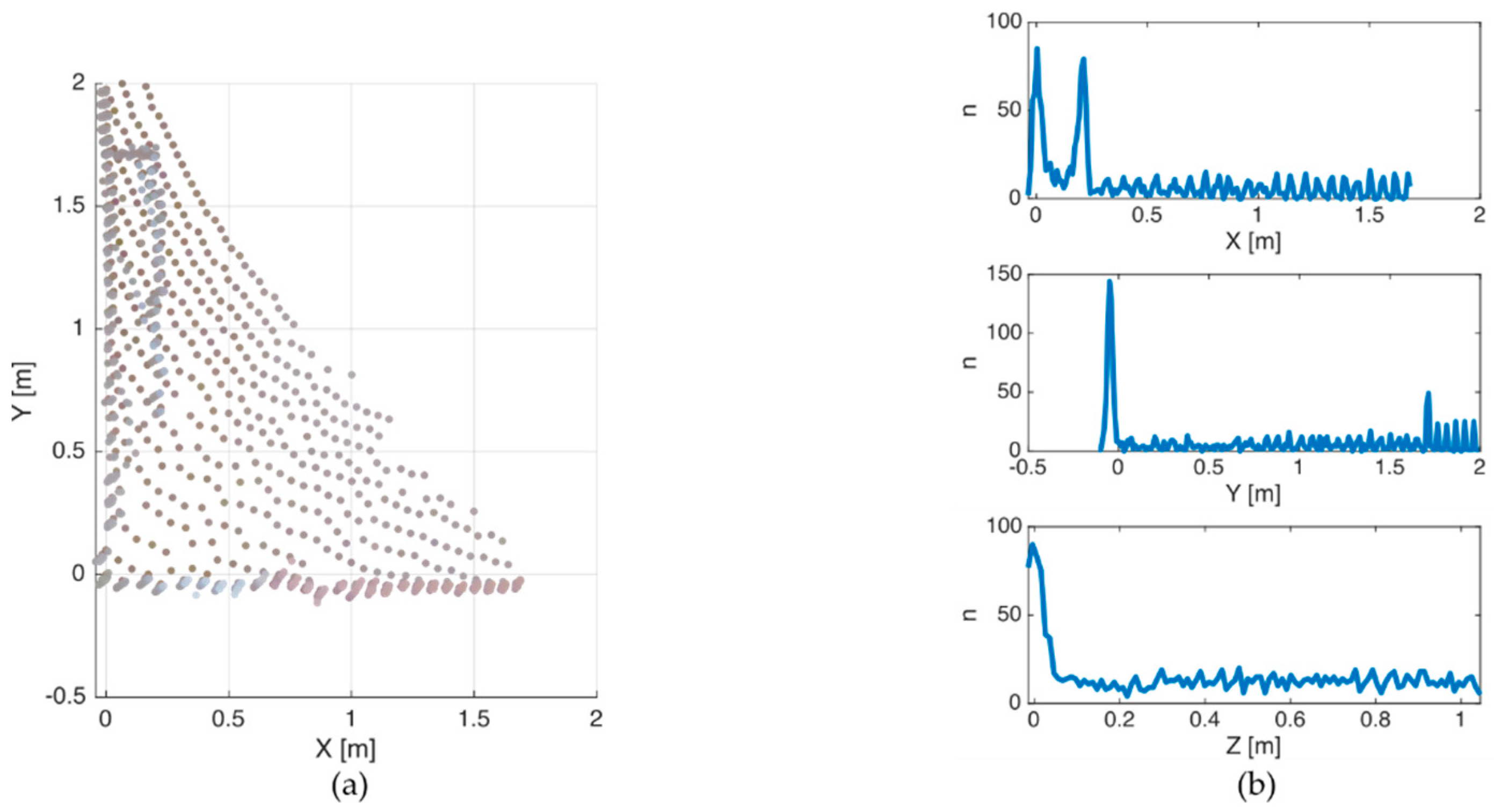
Positions of both maxima are somewhat different. The searched orientation angle $\phi [{}^{°}]$ is the average value of both maxima positions. For this example, the maximum for X-axis in Figure 8a is 3.5 degrees and the maximum for the Y-axis in Figure 8b is 4.7 degrees. Then, the orientation angle is $\phi [{}^{°}]$ = 4.1 degrees. Figure 9 shows the corrected point cloud from Figure 5 including the final histograms. The new histograms in Figure 9b are sharper and have several bigger local maxima in the X and Y axes in comparison to Figure 5b. The histogram in the Z-axis is the same.

The range of the rotation interval $R_{\phi }$ is not possible to select arbitrarily. When a point cloud is rotated in an angle of 90 degrees, then, the X-axis becomes the Y-axis. The universal solution is to determine the initial point cloud rotation as the 0 degrees and the rotation range $R_{\phi }=\pm 45$ degrees. This algorithm is also fast because it uses a classical histogram, which its ways depend on the number of steps. The algorithm estimated the rotation angle ${\phi }_o$ in 10 ms for the used range of angles $R_{\phi }$. As was mentioned above, this algorithm allows the finding of the point cloud rotation of one coordinate axis from the other two. The assumptions for its success are the presence of flat surfaces, which is typically valid for indoor spaces.

5. Planar Surface Detection Algorithm

The known orientation angle of a point cloud allows the detection of planar surfaces in all coordinate axes directly by using only three passes for each axis. More details about the LCCL algorithm are described in papers [29,30,32]. In short, there are two important parameters: the $lvlS$ as the maximal deviation from a level value and the $lvlRS$ multiplier denoting the new level searching range. The algorithm scans a selected coordinate axis by the global virtual plane, which covers the whole horizontal range of the selected axis. The following figures (Figure 10, Figure 11 and Figure 12) illustrate the planar surface detection by using the LCCL algorithm and level image in the X, Y and Z axes respectively.

The width of the analyzed data is defined as the $lvlS\cdot lvlRS$ and from the selected range, a level $dL$ with the highest concentration is found by using the histogram. The range of the detected level is defined as $dL\pm lvlS$. We also developed the algorithm for finding the fine range described in reference [32]. The Figure 10c,d nicely illustrates the planar surface detection of the radiator and the erasing of the selected undesired points by the morphological open. The thickness of the undesired points is smaller than the used element.

The range for the next level estimation is selected from the last $dL+lvlS$ and the same range $lvlS\cdot lvlRS$ used above. This way of selection and using the histogram for finding the highest point concentration allows finding all uniformly distributed flat surfaces in the analyzed point cloud.

The LCCL algorithm itself is not sufficient for planar surface detection. As in Figure 10c, Figure 11c and Figure 12c, from each founded level $dL$, the $I_L$ is created by using the point space quantization parameter $qD.$ For this testing purpose, $qD$ = 4 cm, $lvlS$ = 5 cm and $lvlRS$ = 2.5 are selected. The $I_L$ is firstly processed by the morphological operations and the all planar surfaces are found by the level connected component labeling algorithm. Searching of all levels in all coordinate axes took about 80 ms. The main advantage of $I_L$ is the definite physical position determination of each pixel in space. The processing $I_L$ allows the filling of these missing data. The proposed method is described in the next section.

6. Fill Gaps in Measurement Data

During the planar surface detection process, there can be a requirement for the area determination including the inner holes. This situation occurs mainly when we process the floor or the ceiling areas. The point cloud with missing points on the floor is shown in Figure 13. This example describes the first level estimation in the Z-axis. During the point cloud analysis, there can be the assumption, that the floor is compact and we have a requirement to estimate the area of the floor. The use of $I_L$ for point cloud processing offers the application of wide range image processing algorithms, which help with the important unknown parameter determination in the analyzed point cloud.

The $I_L$ in Figure 13c contains undesired holes, which are possible to fill easily by the use of image processing methods. We used the binary image and connected component labeling algorithm for the filling of the presented holes. The pseudo-code of the proposed algorithm is shown in Algorithm 1.

Algorithm 1. Fill Element Area

Input: Image level element $I_L{E}_x$

Output: Filled element $I_{Efill}$

1 $E_{xB}$ = ElementBorderPositions ($I_L{E}_x$)

2 $E_{xBe}$ = Extend $E_{xB}$ borders about 1 px

3 $I_{one}$ = true(size($E_{xBe}$))

4 $I_{one}$($E_{xBe}$ > 0) = false

//find separate areas (1 - surroundings, 2 - filled element)

5 $L$ = ConnectedComponentLabeling($I_{one}$, 4)

//add edges back

6 $I_{Efill}$ = ($L$ = 2) | $E_{xBe}$

7 $I_{Efill}$ = Narrow $I_{Efill}$ borders about 1 px

The level image consists of several elements representing individual planar surfaces in general. The analyzed element index is marked as $I_L{E}_x$. By using the algorithm for the element borders detection, presented in our previous work [30], the borders of the element $E_{xB}$ are extracted. The algorithm uses erasing of the eroded element by about one pixel from the original element for the border finding. It is necessary to extend the binary image borders by at least about one pixel $E_{xBe}$ for the preserving of the indexing elements expected in further processing. Then, the second image $I_{one}$ of the same size with all values equal to one is created. On the detected border, positions are set to zeros, as shown in the following equation:

$$I_{one}\left(E_{xBe}=1\right)=0.$$

(7)

The connected component algorithm with the connection of four is applied to the obtained image. The connection of eight is not possible to use because the border width is only one pixel thin and in the diagonal directions the algorithm may cross the borders. The result of labeling $L$ is two areas with different indexes. Index 1 is the surroundings, and index 2 is the desired filled area without borders. By adding the borders of the analyzed element to the labeled area by the index 2, the original filled area is obtained as:

$$I_{Efill}=(L=2)\vee E_{xBe}$$

(8)

The extension of one pixel is erased for the getting of the original level image size. Figure 13d gives the final filled area, which is calculated from the original floor elements with the holes. The filled planar surface allows estimation of the real floor area or the space volume like in Section 8 with the results. We can reconstruct the missing points by the reverse process from the fixed floor planar surface. Moreover, from the difference of Figure 13c,d, it is possible to reconstruct only the missing parts and with the knowledge of planar surface statistical parameters, we can generate the missing points with the same statistical distribution.

7. Vectorization of Basic Space Features

One of the point cloud processing aims is the decreasing of descriptive points. The meaning of the term vectorization is to describe a shape by the vertices points. For example, the knowledge of all border positions of pixels is unnecessary, only the vertices points are important for reconstruction of the shape, as is shown in Figure 13d.

The proposed method for finding the vertices points is based on our presented method for the perimeter estimation (see reference [30]). Figure 14 illustrates the way how to determine the perimeter of a shape.

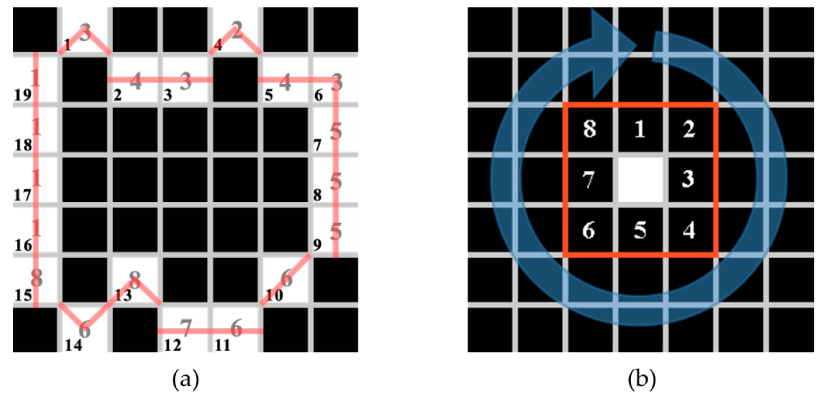
The perimeter is not possible to determine as simply as the area by multiplication of the count of border pixels. Borders are extracted in the same way as in Algorithm 1. The additional analysis of these borders is necessary for precise perimeter estimation. We need to determine the direct and diagonal path of the perimeter. This mentioned problem solves the modified connected component algorithm for the determination of these borders, including the record of the searching direction of connected pixels, the perimeter path $P_p$. The algorithm uses a different mechanism of searching connected pixels, see Figure 14b. When the first border pixel $n$ is found, the neighbor pixel $(n+1)$ is searched in the direction denoting the numbers in Figure 14b. When the neighbor pixel $(n+1)$ is found, the actual searching ends. The pixel $(n+1)$ becomes the pixel $n$ and the searching continues in the same way until all pixels of the border are found. For the direct pixel path, there are numbers 1, 3, 5 and 7 and their length is pixel size. Numbers 2, 4, 6 and 8 are used for the diagonal direction and their length is equal to the diagonal of one pixel. We also watch the score function in the Y-axis determining the position of the last pixel of the round perimeter against the first pixel of the perimeter. For more details, see paper [30]. Figure 14a gives the example of all possible occurrences of directions during the perimeter pixels searching. The optimal perimeter is marked by the light red color line. The number in the corner is the border pixel order and the bigger numbers are directions of their detection. The difference of the perimeter estimation in this simple example with consideration of diagonal direction against the simple pixel multiplication is 10%.

We developed the algorithm for the shape vertices points extraction represented by a level image from the known history of the searching path $P_p$, the score function $Y_s$ and round perimeter condition. The pseudo-code is shown in Algorithm 2.

Algorithm 2. Element Vertices Extraction

Input: Perimeter path $P_p$;

Score function in the Y axis $Y_s$

Condition of circle perimeter $cirP$

Output: Vertices of element $cPos$

1 $c{P}_i=0$

2 $cPos$($c{P}_i$++,∀) = [$P_p$(1), 1]

3 for each $P_p$(n) $\in$ $P_p$ from n = 2 do

4     if($cPos$($c{P}_i$, 1) $\ne P_p$(n)) then

5       //last position before change

6       $cPos$($c{P}_i$++,∀) = [$P_p$(n − 1),n − 1]

7       //actual position

8       $cPos$($c{P}_i$++,∀) = [$P_p$(n),n]

9     end

10 end

11 Exclude repeated items in $cPos$

12 if ($cirP$ && $Y_S>0$) then

13  Remove $cPos$($end,$ ∀)

14 end

The vertices positions are stored in the array $cPos$. The first found border direction is written into this array. The next step is searching through the whole history of the direction path $P_p$ from the index $n=2$. The algorithm focuses on indexes with a change of path direction against the last found vertex $c{P}_i$. When the direction change is detected, the actual path direction on $n$ position is stored including the border position index. The corresponding values on position $(n-1)$ are stored too. The reason for this is obvious in Figure 14a. For example, the direction change from 5 to 6 of the 9^th pixel is detected on pixel 10, but the vertex is just pixel 9. After the $P_p$ searching, the doubled directions occur in $cPos$ array, for example, the pixels 7 and 9 or 10 and 11. The first position of doubled directions is removed. The last step of the algorithm is the decision about the last position of $P_p$. The last pixel position against the first has to be determined for the round border defined by $cirP$. When the score function $Y_s$ is higher or equal to one, the last pixel connection with the first is diagonal. Then, the last item $P_p$ is added. The last item $P_p$ is excluded for the diagonal direction longer than one pixel. The detection of vertices for the test images of Figure 14a and Figure 13d are illustrated in Figure 15a and in Figure 15b respectively.

The red pixels are detected vertices of the input level image. The compact version of the level image in Figure 14a is created from 39 pixels and only 13 pixels describe vertices of the shape. The origin image in Figure 13d is composed of 961 pixels and 67 vertices were found. The presented method is valid for the compact level images. When some holes are present in an image, the image can be binary inverted. The complete vertices description of a shape (including the holes) is available if we determine also the vertices of the holes.

8. Results

Our previous papers [29,30,31] usually show the point cloud processing only of a single room. In this paper, we decide to show processing of the entire flat. All blocks from the processing scheme in Figure 1 were used. This section is divided into four subsections: in the first, our optical rangefinder is briefly described; the second focused on the used input point cloud representing the real flat with three rooms and one corridor, this subsection also describes its scanning process and the complex output point cloud construction; the next subsection presents obtained results by using the developed processing pipeline; and the last evaluates the algorithms in detail in terms of the precision and possibilities of using.

8.1. Optical Rangefinder for Space Scanning

As the remote sensing device for space scanning, we used our developed optical rangefinder. The described 3D range scanning system is part of a bigger project called ARES (Autonomous Research Exploration System), which is described in references [33,34]. The rangefinder sweeps a laser point into the vertical line and in each point of this line, it is possible to estimate the point position in the space. The measurement principle is based on the triangle similarity described in reference [35]. For detailed information on how to determine a 3D point in a scanned space, see references [35,36]. The whole measuring device consists of a tripod; a high-quality Basler color camera with a resolution of 2590 × 1942 pixels; a green 200 mW laser diode; an optical filter with an angle of 90 degrees for vertical swapping of the laser beam; and a fast and powerful stepping motor for 360 degrees rotation. The following figure shows the practical measurement Figure 16a with measurement frame Figure 16b.

We replaced the used camera lens with a lower focal length to cover a higher range in the height during the development of this device. The lower focal length caused the undesired barrel distortion effect. This effect elimination is described in reference [37]. In one of our recent papers ([38]), we developed the automatic algorithm for the best undistortion parameter estimation. The laser line is segmented from a static measurement frame by the HSV GMM (Gaussian Mixture Model). The HSV color model best covers the intensity range of the used laser (see references [39,40]). The intensity of laser pixels in the measurement image depends on the distance from a scanning object and its reflection of the laser spectrum. Nevertheless, in the measured frames, pixels with a low and high intensity similar to the spectrum of a laser or reflected laser light can occur. For the robustness of the position determination and distinguishing from a laser colored object, it is important to analyze, the laser pixel intensity as well as the laser element shape. A statistical analysis of both parameters offers to detect the main laser line intensity correctly. More details about the best laser element selection and the main laser intensity estimation is described in references [41,42]. We also implemented the fusion of image data from the camera with points in space to achieve a colored point cloud by using a template matching method in two measurement frames (see reference [36]). The measurement system can determine the vertical laser line with a half-pixel accuracy. The accuracy of the distance determination for the actual rangefinder configuration is shown in Figure 17.

The maximal error is 3.5% in the range of 15 m. In the bigger distances, the laser line is closer to a measurement frame center, and the change of position of about one pixel causes a bigger change in the measurement distance. This dependency is non-linear and causes bigger measurement errors. More about this non-linearity and calibration of the optical rangefinder is described in reference [43]. In comparison with the present expensive professional laser scanners, our rangefinder can be labeled as a home 3D scanner.

8.2. Input Point Cloud

As a scanning space, we selected an indoor space, a flat. There are three rooms and one corridor in this flat. To cover the whole space, we placed our optical rangefinder on eight measurement positions. Individual positions are marked in the top view flat scheme in Figure 18b. The room with positions 3 and 4 is the kitchen. All constructed output point clouds are shown in Figure 18a. The green numbers in brackets are equal to the measurement positions. Differences in the color intensity in Figure 18a are caused by the different light conditions during the scanning process. The complete composed point cloud of the flat is shown in Figure 18c.

For the register of the individual point clouds, we used the NTD (Normal Distribution Transform) registration algorithm, which is implemented in the PCL (Point Cloud Library) described in reference [44]. This colored point cloud provides an overview of the scanned space, and from coordinate axes, we can estimate the basic size. However, to obtain the important features of the other space, further processing is needed. The presented point clouds in Figure 18a are clear of outlier points. These points have an influence on the registration process and their removing must be done before the registration process. For their elimination, we proposed the algorithm based on the histogram of a point density in the individual coordinate axes. The algorithm is described in Section 3.

The outlier points were removed from each scan after the scanning from the eight measurement positions. Then, the output point cloud of the flat was composed by the NDT registration process. The initial angle rotation of −3.15 degrees was detected by the algorithm presented in Section 4 from the final point cloud. The algorithm estimated the initial rotation angle in 3.35 s.

The preprocessed space data can be analyzed further in terms of the object detection and physical space description described in Section 7, Section 8 and Section 9. The knowledge of the initial rotation angle allows the detection of the planar surfaces in all coordinate axes by our proposed LCCL algorithm with only three passes. The point cloud rotation in a prescribed range of angles and finding the best match of points in detected planar surfaces for the complex plane detection with all possible orientation angles can be realized according to [29]. Searching of all levels in all coordinate axes took about 1.5 s.

8.3. Processing Results

Table 1. Detection parameter for all coordinate axes.

Axis	lvlS	lvlRS	qD
X	0.1 m	2.5	4 cm
Y	0.1 m	2.5	4 cm
Z	0.2 m	1.5	4 cm

summarizes the used detection parameters for all coordinate axes. The detection parameter selection depends on the quality of a used 3D scanner.

In our case, due to the worse scanner calibration, the range $lvlS$ is higher. We can choose a bigger value of $lvlS$ and $lvlRS$, if we do not expect parallel surfaces close to each other in the selected range $lvlS\cdot lvlRS$. The level $dL$ detection by the histogram will always find the highest point concentration. In following Figure 19, the visualization of the flat by our proposed processing is shown with the utilization of the level image, allowing also the plane visualization (see reference [31]). The orientation of the planar surfaces is marked by three colors according to the surface orientation (X, Y, and Z).

The detected planar surfaces with their physical parameters are described in the following tables (

Table 2. Detected planes with the physical description in the X-axis.

Idx	dL (m)	Pos (m)	AE (m2)	PE (m)	$\mathit{\sigma }$ (m)	PC p.	IL px.	V	P. decr.%
2	0.313	0.313, 3.935, 3	7.174	19.33	0.0008	7306	4420	92	98.74
4	3.521	3.52, 3.926, 3	9.862	18.177	0.0018	15,211	6148	71	99.53
5	3.687	3.687, 2.581, 2.88	11.645	21.41	0.0006	14,460	7166	92	99.36
14	7.162	7.162, 2.56, 2.96	13.278	20.833	0.0006	10,687	8112	87	99.19
16	7.371	7.371, 4.454, 2.8	8.754	11.96	0.001	16,025	5450	43	99.73
22	8.917	8.917, 0.291, 2.72	7.15	15.443	0.001	7424	4452	81	98.91

,

Table 3. Detected planes with the physical description in the Y-axis.

Idx	dL (m)	Pos (m)	AE (m2)	PE (m)	$\mathit{\sigma }$ (m)	PC p.	IL px.	V	P. decr.%
1	0.081	3.926, 0.081, 2.88	13.334	15.226	0.0013	22,161	8270	82	99.63
7	2.647	3.653, 2.647, 2.92	9.7856	12.4	0.0008	13,456	6054	49	99.64
10	3.949	0.135, 3.949, 2.96	10.026	12.69	0.0007	14,802	6192	39	99.74
14	4.497	7.115, 4.497, 2.80	7.7008	16.89	0.0009	9847	4748	85	99.14
29	7.819	0.271, 7.819, 3.12	21.661	35.236	0.0018	26,529	13840	162	99.39

and

Table 4. Detected planes with the physical description in the Z-axis.

Idx	dL (m)	Pos (m)	AE (m2)	PE (m)	$\mathit{\sigma }$ (m)	PC p.	IL px.	V	P. decr.%
1	0.023	0.262, 0.018, 0.023	55.835	45.643	0.006	14,223	34,897	270	98.1
4	0.987	0.091, 3.936, 0.987	0.76	4.61	0.010	2673	475	36	98.65
6	0.942	4.415, 7.593, 0.942	0.739	4.537	0.014	1710	462	21	98.77
8	0.926	8.013, 5.763, 0.926	1.845	9.8	0.012	6629	1153	58	99.13
12	1.353	10.129, 5.853, 1.353	0.773	4.96	0.009	2555	483	22	99.14
21	2.956	0.102, 0.012, 2.672	59.246	39.319	0.019	16,173	37,029	162	99

). Presented planes in the X- and Y-axis have an area bigger than 5 m². The attributes denote from the left side: Idx—the detection level index; dL—the detected level in the scanned dimension; Pos—the coordinates of the image level origin in the space; A_E the area of the planar surface plane; P_E the perimeter of the plane; $\sigma$—the standard deviation of the points forming the planar surface; PC p.—the number of points representing the planar surface; I_L px—the count of level image pixels; V—vertices of the plane; and P. decr.% expressing the decrease between the number of found vertices and the original points of the plane.

We can notice from the analysis of the tables, that indexes 4, 5 and 14, 16 in Table 2 show the ability of the scanning algorithm to detect parallel walls. The last row in all tables shows how many percentages of storage can be saved if we present a planar surface only by their vertices. The first planar plane surface in Table 3 is the floor of the flat. We can express the volume of the flat as the known area multiplied by the height of the flat. The planar surface 21, detected in the level 2.956 m, is the ceiling in Table 3. Then, the volume of the flat is approximately 165 m³.

The obtained results show the advantages of the proposed processing. By using the level image, it is possible to easily express the statistical parameters of the represented planar surface, process plane visualization, and decrease the number of points necessary for the planar surface description. The presented algorithms were tested on the CPU i5-2410M 2,3 GHz. The input point cloud consists of 219,216 points and the detection time of all planar surfaces is not higher than three seconds.

The mentioned algorithms in Section 1 can be used for the detection of planar surfaces. Then, the segmented raw point cloud of a planar surface can be processed by our proposed approach utilizing a level image with the connection of image processing methods. This concept allows us to easily get the important physical space properties, decrease the descriptive point amount, or visualize the planar surface.

The following tables (

Table 5. Physical area and perimeter, difference in percent (X-axis).

Idx	AE (m2)	A phys (m2)	Δ A (%)	PE (m)	P phys (m)	Δ P (%)
2	7.174	6.97	2.84	19.33	18.95	1.97
4	9.862	8.976	8.98	18.177	16.856	7.27
5	11.645	11.728	0.71	21.41	21.68	1.26
14	13.278	13.489	1.59	20.833	21.34	2.43
16	8.754	8.28	5.41	11.96	11.22	6.19
22	7.15	6.95	2.80	15.443	15.133	2.01

,

Table 6. Physical area and perimeter, difference in percent (Y-axis).

Idx	AE (m2)	A phys (m2)	Δ A (%)	PE (m)	P phys (m)	Δ P (%)
1	13.334	12.45	6.63	15.226	14.92	2.01
7	9.7856	10.26	4.85	12.4	12.76	2.90
10	10.026	10.12	0.94	12.69	12.78	0.71
14	7.7008	7.43	3.52	16.89	16.27	3.67
29	21.661	22.3	2.95	35.236	36.44	3.42

and

Table 7. Physical area and perimeter, difference in percent (Z-axis).

Idx	AE (m2)	A phys (m2)	Δ A (%)	PE (m)	P phys (m)	Δ P (%)
1	55.835	54.32	2.71	45.643	44.28	2.99
4	0.76	0.79	3.95	4.61	4.86	5.42
6	0.739	0.712	3.65	4.537	4.33	4.56
8	1.845	1.765	4.34	9.8	9.45	3.57
12	0.773	0.81	4.79	4.96	5.15	3.83
21	59.246	56.392	4.82	39.319	38.507	2.07

) give the percentage difference between the real physical area and perimeter in each coordinate axis. Columns marked by $phys$ determine the physical values. The estimated values directly reflect the level image content which depends mainly on the objects covering by measurement points.

When we compare the percentage values, it is noticeable that some planar surfaces were segmented correctly, where the error is lower than 3%. Few planar surfaces have the difference between the estimated and physical value close to 10%. These cases indicate a worse covering by the measurement points. As it will be shown in the next subsection, our developed approach reflects the real input data content.

For the robust results evaluation, we also compared the physical results with the convex hull method. The next tables (

Table 8. Physical area and perimeter, difference in percent from convex hull (X-axis).

Idx	ACH (m2)	A phys (m2)	Δ A (%)	PCH (m)	P phys (m)	Δ P (%)
2	11.461	6.97	39.19	13.338	18.95	42.08
4	11.425	8.976	21.44	13.38	16.856	25.98
5	14.121	11.728	16.95	15.343	21.68	41.30
14	14.948	13.489	9.76	15.632	21.34	36.51
16	9.1922	8.28	9.92	11.919	11.22	5.86
22	8.3255	6.95	16.52	11.031	15.133	37.19

,

Table 9. Physical area and perimeter, difference in percent from convex hull (Y-axis).

Idx	ACH (m2)	A phys (m2)	Δ A (%)	PCH (m)	P phys (m)	Δ P (%)
1	13.494	12.45	7.74	14.693	14.92	1.54
7	9.8345	10.26	4.33	12.294	12.76	3.79
10	10.231	10.12	1.08	12.342	12.78	3.55
14	9.5068	7.43	21.85	11.878	16.27	36.98
29	29.797	22.3	25.16	25.862	36.44	40.90

and

Table 10. Physical area and perimeter, difference in percent from convex hull (Z-axis).

Idx	ACH (m2)	A phys (m2)	Δ A (%)	PCH (m)	P phys (m)	Δ P (%)
1	69.044	54.32	21.33	32.062	44.28	38.11
4	0.938	0.79	15.78	5.07	4.86	4.23
6	0.789	0.712	9.76	4.60	4.33	5.80
8	4.033	1.765	56.24	8.40	9.45	12.52
12	0.948	0.81	14.56	4.92	5.15	4.61
21	71.703	56.392	21.35	32.786	38.507	17.45

) give the percentage difference form the real physical values. Columns marked by $CH$ determine the area and perimeter by the convex hull.

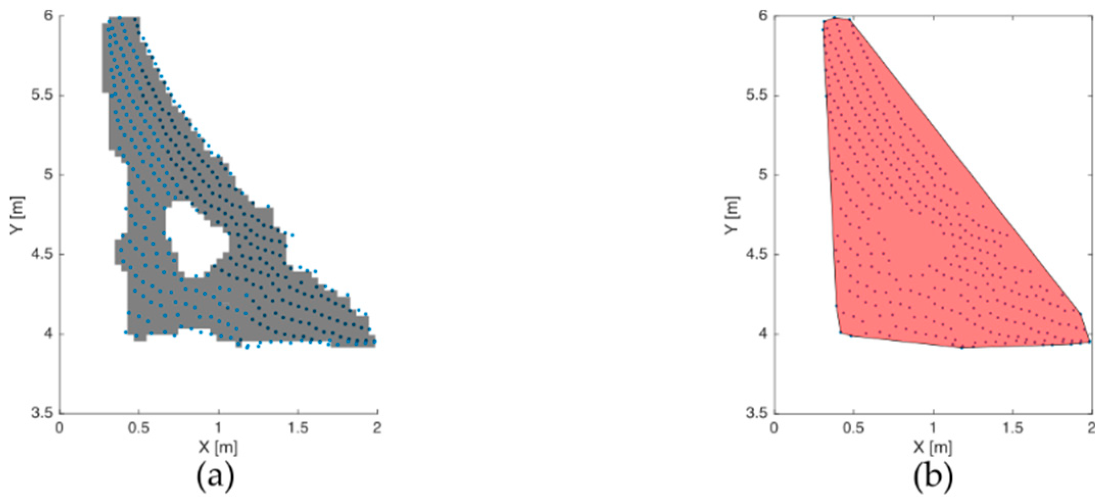
The comparison of both tables (Table 5, Table 6 and Table 7) with (Table 8, Table 9 and Table 10) shows that in several cases the percentage difference is in units of percent. Even in four cases, the convex hull method overcomes our method in the determination of at least one compared value. However, in many cases, the difference is even more than 15%. This is caused by the convex hull nature to find the smallest convex polygon that has no corner bent inwards, as shown in following Figure 20. For simple compact planar shapes as squares, rectangles, triangles, and similar shapes without corners bent inwards, this method gives precise results. This assumption is not usually valid in real environments.

Figure 20b shows the problem of finding the convex polygon that has no corner bent inwards. Additionally, the convex hull does not detect holes as Figure 20a illustrating the detection by the level image. Instead of the area and perimeter determination, the level image has also features to detect holes, segment all planar surfaces in one detected level and express statistical properties of a planar surface. The precision of the level image depends mainly on the suitable selection of quantization parameter $qD$. The most important advantage of a level image is the planar surface representation in the different form, allowing the using of image processing methods. This offers to use the wide range methods to get important planar surface properties. The mathematical solution for complex shapes can be difficult. The image presentation offers to analyze also the depth information, which can be used to detect 3D shapes in the future.

8.4. Evaluation of Processing Algorithms

Following Figure 21 shows the planar surfaces visualization by using the level images from Figure 13c,d. The level images were achieved by the LCCL algorithm. For a better illustration, the segmented points are also included. From both visualizations, it is obvious the good covering of all points. From this follows that the results of the developed algorithms strongly depend on the quality of an input point cloud.

The results of the planar surface segmentation can be improved by the fine segmentation, as we introduced in reference [32]. Figure 22 gives an example of the usage for the level detection in Figure 10. For the processing of the final point cloud composing the flat, we did not use this fine ranging. Figure 22d shows the problematic case. The noisy curve is the histogram of the points representing a level in the scanning dimension ${\dim }_s$. The green line is the moving average of the histogram with the selected window size 1 cm. From the filtered curve, it is possible to surely estimate positions of both elbows, where the derivation is smaller than the desired threshold. For example, due to measurement errors and the worse result of the registration process, points from two scans covering one wall can be slightly shifted and two local maxima of points concentration can be close to each other. When this situation occurs, the algorithm ends with a similar result as in Figure 22d. This can lead to the detection of double walls.

For this reason, it is better to not use this approach on data with measurement errors. Prior information about the point cloud data quality or the demands on the planar surface detection is desirable. We are focusing on the two main parameters, the expected standard point deviation from a detected planar surface and the minimal distance between two planar surfaces in the direction of analyzing individual levels. This reflects the selection of the parameters $lvlS$ and $lvlRS$. The $lvlS$ value also expresses the expected standard point deviation from a planar surface. If this parameter is set too high, the two close planar surfaces can be detected as one. The higher $lvlRS$ value selection is always recommended, as this ensures the sufficient data range selection in the scanning dimension and the histogram of points concentration will find the best probability of a level position for a planar surface presence. To ensure the probability that a point belongs to the best planar surface, we can follow the statistical parameters of all planar surfaces.

Next, Figure 23 shows the possibility of using the level image for the point cloud segmentation. For a level image, its physical origin in space, orientation angle, and quantization parameter are known. From this, we can easily extract desired points as shown in this example.

The next advantage lies in the extensibility of well known point cloud processing methods mentioned in Section 1. A segmented planar surface can be further processed by our developed algorithms. Following Figure 24 shows the segmentation of different planar surfaces. When we are processing data, we can also focus only on planar surfaces with the desired parameters as the area, perimeter, shape, or for example a planar surface variance, see Figure 24. It is necessary to mention that the flat from Figure 19 is empty of furniture except for the kitchen units. Even if some furniture is present in the scanning scene, we can detect all present planar surfaces. The presented point cloud processing pipeline detects, presents, and reflects all what it is physically present in input data. The use of this proposed processing concept is wide.

9. Conclusions

In this paper, we presented several methods for point cloud processing from basic preprocessing, such as removing outlier points, initial rotation angle estimation against base coordinate axis to the point cloud simplification, and global space parameter estimation. The main assumption for its success depended on planar surface presence in analyzed data, which is highly probable and almost every time fulfilled in an indoor space. The results of these methods are summarized in the following three points:

• Outliers and rotation—The simple point concentration histogram offers to remove outliers. This improved the result of the final point cloud composition by the registration process. Moreover, the thoroughly selected processing of histograms in the two axes allows the relatively fast finding of the initial point cloud orientation against the third coordinate axis. This is mainly important for the decreasing processing time. Only three passes of the scanning algorithms allow finding of all planar surfaces in each coordinate axis as documented in the tables of results.
• Holes removing—The composed point cloud from several scans may lack of points in some part of the presented surfaces. The filling of holes in a level image representing a planar surface makes it possible to reconstruct the missing points. The filled holes allow the estimation of the real surface area. It makes even it possible to estimate the volume of a space when its height is known in the case of the floor or ceiling.
• Simplification of objects—The proposed approach showed the successful planar surface detection in the desired coordinate axes. It offers alternative point cloud processing and extends the possibilities of the present methods. The scanning algorithm for the planar surface detection allows the description of these planar surfaces by the statistical parameters. The standard deviation of the detected planar surfaces is small, which indicates their precise detection, as was shown in the capture results. We can see that thanks to this, it is easy to possibly detect the parallel walls. The presentation of planar surfaces by the level images offers to estimate important space properties as the area and perimeter. The image processing methods allow easy determination of these parameters against the difficult mathematical solution for the irregular shapes. All the detected properties make it possible to classify each planar surface. The results also show the ability of the algorithm for the descriptive point decreasing. All the planar surfaces presented only by their vertices showed a 99% decrease in points almost in all cases.

Moreover, all features of the proposed processing pipeline are usable not only for point clouds, but they are valid for the detection and analysis of different levels for any 3D data in general. Future research will focus on object detection and tracking. The planar surfaces representation allows removal of the scanned space boundary and extracts only the desired objects. The analysis of the level of image shape can be used to categorize objects into groups. The extension of the level image content in more depth can offer the categorization of 3D objects. The next possible way is to create the simulator based on the measured data, which will create the training spaces with some targets, and this can be used for neural networks training.

References

1. Berger, M.; Tagliasacchi, A.; Seversky, L.M.; Alliez, P.; Levine, J.A.; Sharf, A.; Silva, C.T. State of the Art in Surface Reconstruction from Point Clouds. Eurographics 2014, 161–185. [Google Scholar] [CrossRef]
2. Ochmann, S.; Vock, R.; Klein, R. Automatic reconstruction of fully volumetric 3D building models from oriented point clouds. ISPRS J. Photogramm. Remote Sens. 2019, 151, 251–262. [Google Scholar] [CrossRef] [Green Version]
3. Mura, C.; Mattausch, O.; Jaspe Villanueva, A.; Gobbetti, E.; Pajarola, R. Automatic room detection and reconstruction in cluttered indoor environments with complex room layouts. Comput. Graph. 2014, 44, 20–32. [Google Scholar] [CrossRef] [Green Version]
4. Jain, S.; Argall, B. Estimation of Surface Geometries in Point Clouds for the Manipulation of Novel Household Objects. In Proceedings of the RSS 2017 Workshop on Spatial-Semantic Representations in Robotics, Cambridge, MA, USA, 12–16 July 2017; Robotics Science and Systems: Corvallis, OR, USA, 2017. [Google Scholar]
5. Zhao, R.; Pang, M.; Liu, C.; Zhang, Y. Robust Normal Estimation for 3D LiDAR Point Clouds in Urban Environments. Sensors 2019, 19, 1248. [Google Scholar] [CrossRef] [Green Version]
6. El-Sayed, E.; Abdel-Kader, R.F.; Nashaat, H.; Marei, M. Plane detection in 3D point cloud using octree-balanced density down-sampling and iterative adaptive plane extraction. IET Image Process. 2018, 12, 1595–1605. [Google Scholar] [CrossRef] [Green Version]
7. Czerniawski, T.; Sankaran, B.; Nahangi, M.; Haas, C.; Leite, F. 6D DBSCAN-based segmentation of building point clouds for planar object classification. Autom. Construct. 2018, 88, 44–58. [Google Scholar] [CrossRef]
8. Xu, X.; Luo, M.; Tan, Z.; Zhang, M.; Yang, H. Plane segmentation and fitting method of point clouds based on improved density clustering algorithm for laser radar. Infrared Phys. Technol. 2019, 96, 133–140. [Google Scholar] [CrossRef]
9. Zhang, Y.; Lu, T.; Yang, J.; Kong, H. Split and Merge for Accurate Plane Segmentation in RGB-D Images. In Proceedings of the 4th IAPR Asian Conference on Pattern Recognition (ACPR), Nanjing, China, 26–29 November 2017; IEEE: Piscataway, NJ, USA, 2017; pp. 49–54. [Google Scholar] [CrossRef]
10. Jin, Z.; Tillo, T.; Zou, W.; Zhao, Y.; Li, X. Robust Plane Detection Using Depth Information from a Consumer Depth Camera. IEEE Trans. Circuits Syst. Video Technol. 2019, 29, 447–460. [Google Scholar] [CrossRef]
11. Vera, E.; Lucio, D.; Fernandes, L.A.F.; Velho, L. Hough Transform for real-time plane detection in depth images. Pattern Recognit. Lett. 2018, 103, 8–15. [Google Scholar] [CrossRef]
12. Skulimowski, P.; Owczarek, M.; Strumiłło, P. Ground Plane Detection in 3D Scenes for an Arbitrary Camera Roll Rotation Through “V-Disparity” Representation. In Proceedings of the Federated Conference on Computer Science and Information Systems, Prague, Czech Republic, 3–6 September 2017; IEEE: Piscataway, NJ, USA, 2017; pp. 669–674. [Google Scholar] [CrossRef] [Green Version]
13. Phalak, A.; Chen, Z.; Yi, D.; Gupta, K.; Badrinarayanan, V.; Rabinovich, A. DeepPerimeter: Indoor Boundary Estimation from Posed Monocular Sequences. arXiv 2019, arXiv:1904.11595. [Google Scholar]
14. Guerrero, P.; Kleiman, Y.; Ovsjanikov, M.; Mitra, N.J. PCPNet Learning Local Shape Properties from Raw Point Clouds. Comput. Graph. Forum 2018, 37, 75–85. [Google Scholar] [CrossRef] [Green Version]
15. Griffiths, D.; Boehm, J. Improving public data for building segmentation from Convolutional Neural Networks (CNNs) for fused airborne lidar and image data using active contours. ISPRS J. Photogramm. Remote Sens. 2019, 154, 70–83. [Google Scholar] [CrossRef]
16. Beksi, W.J.; Papanikolopoulos, N. A topology-based descriptor for 3D point cloud modeling: Theory and experiments. Image Vis. Comput. 2019, 88, 84–95. [Google Scholar] [CrossRef]
17. Liu, X.; Zhang, Y.; Ling, X.; Wan, Y.; Liu, L.; Li, Q. TopoLAP: Topology Recovery for Building Reconstruction by Deducing the Relationships between Linear and Planar Primitives. Remote Sens. 2019, 11, 1372. [Google Scholar] [CrossRef] [Green Version]
18. Lian, X.; Hu, H. Terrestrial laser scanning monitoring and spatial analysis of ground disaster in Gaoyang coal mine in Shanxi. Environ. Earth Sci. 2017, 76, 287. [Google Scholar] [CrossRef]
19. Drews, T.; Miernik, G.; Anders, K.; Höfle, B.; Profe, J.; Emmerich, A.; Bechstädt, T. Validation of fracture data recognition in rock masses by automated plane detection in 3D point clouds. Int. J. Rock Mech. Min. Sci. 2018, 109, 19–31. [Google Scholar] [CrossRef]
20. Nguyen, H.L.; Belton, D.; Helmholz, P. Planar surface detection for sparse and heterogeneous mobile laser scanning point clouds. ISPRS J. Photogramm. Remote Sens. 2019, 151, 141–161. [Google Scholar] [CrossRef]
21. Jiang, Y.; Li, C.; Takeda, F.; Kramer, E.A.; Ashrafi, H.; Hunter, J. 3D point cloud data to quantitatively characterize size and shape of shrub crops. Horticult. Res. 2019, 6, 43. [Google Scholar] [CrossRef] [Green Version]
22. Hu, C.; Pan, Z.; Li, P. A 3D Point Cloud Filtering Method for Leaves Based on Manifold Distance and Normal Estimation. Remote Sens. 2019, 11, 198. [Google Scholar] [CrossRef] [Green Version]
23. Peebles, M.; Lim, S.H.; Streeter, L.; Duke, M.; Au, C.K. Ground Plane Segmentation of Time-of-Flight Images for Asparagus Harvesting. In Proceedings of the International Conference on Image and Vision Computing, Auckland, New Zealand, 19–21 November 2018; IEEE: Piscataway, NJ, USA, 2018; pp. 1–6. [Google Scholar] [CrossRef] [Green Version]
24. Pascu, I.S.; Dobre, A.C.; Badea, O.; Tănase, M.A. Estimating forest stand structure attributes from terrestrial laser scans. Sci. Total Environ. 2019, 691, 205–215. [Google Scholar] [CrossRef]
25. Del-Campo-Sanchez, A.; Moreno, M.; Ballesteros, R.; Hernandez-Lopez, D. Geometric Characterization of Vines from 3D Point Clouds Obtained with Laser Scanner Systems. Remote Sens. 2019, 11, 2365. [Google Scholar] [CrossRef] [Green Version]
26. Lubiw, A.; Maftuleac, D.; Owen, M. Shortest paths and convex hulls in 2D complexes with non-positive curvature. Comput. Geom. 2020, 89, 101626. [Google Scholar] [CrossRef] [Green Version]
27. Chmelar, P.; Beran, L.; Kudriavtseva, N. Projection of Point Cloud for Basic Object Detection. In Proceedings of the ELMAR 2014, Zadar, Croatia, 10–12 September 2014; IEEE: Piscataway, NJ, USA, 2014; pp. 1–4. [Google Scholar] [CrossRef]
28. Chmelar, P.; Beran, L.; Rejfek, L. The Depth Map Construction from a 3D Point Cloud. In MATEC Web of Conferences; EDP Sciences: Les Ulis, France, 2016; Volume 75. [Google Scholar] [CrossRef] [Green Version]
29. Chmelar, P.; Rejfek, L.; Beran, L.; Dobrovolny, M. A point cloud decomposition by the 3D level scanning for planes detection. Int. J. Adv. Appl. Sci. 2017, 4, 121–126. [Google Scholar] [CrossRef] [Green Version]
30. Chmelar, P.; Beran, L.; Chmelarova, N.; Rejfek, L. Advanced Plane Properties by Using Level Image. In Proceedings of the 28th International Conference Radioelektronika (RADIOELEKTRONIKA), Prague, Czech Republic, 19–20 April 2018; IEEE: Piscataway, NJ, USA, 2018; pp. 1–6. [Google Scholar] [CrossRef]
31. Chmelar, P.; Rejfek, L.; Beran, L.; Chmelarova, N.; Dobrovolny, M. Point Cloud Plane Visualization by Using Level Image. J. Fundam. Appl. Sci. 2018, 10, 547–560. [Google Scholar]
32. Chmelarova, N.; Chmelar, P.; Rejfek, L. The Fine Plane Range Estimation from Point Cloud. In Proceedings of the 29th International Conference Radioelektronika (RADIOELEKTRONIKA), Paradubice, Czech Republic, 16–18 April 2019; IEEE: Piscataway, NJ, USA, 2019; pp. 1–5. [Google Scholar] [CrossRef]
33. Beran, L.; Chmelar, P.; Dobrovolny, M. Navigation of Robotic Platform with Using Inertial Measurement Unit and Direct Cosine Matrix. In Proceedings of the ELMAR 2014, Zadar, Croatia, 10–12 September 2014; IEEE: Piscataway, NJ, USA, 2014; pp. 1–4. [Google Scholar] [CrossRef]
34. Beran, L.; Chmelar, P.; Rejfek, L. Navigation of Robotics Platform Using Monocular Visual Odometry. In Proceedings of the 25th International Conference Radioelektronika (RADIOELEKTRONIKA), Paradubice, Czech Republic, 21–22 April 2015; IEEE: Piscataway, NJ, USA, 2015; pp. 213–216. [Google Scholar] [CrossRef]
35. Chmelar, P.; Dobrovolny, M. The Fusion of Ultrasonic and Optical Measurement Devices for Autonomous Mapping. In Proceedings of the 23rd International Conference Radioelektronika (RADIOELEKTRONIKA), Paradubice, Czech Republic, 16–17 April 2013; IEEE: Piscataway, NJ, USA, 2013; pp. 292–296. [Google Scholar] [CrossRef]
36. Chmelar, P.; Beran, L.; Rejfek, L.; Chmelarova, N. The Point Cloud Visualisation for Rotary Optical Rangefinders. In Proceedings of the 27th International Conference Radioelektronika (RADIOELEKTRONIKA), Brno, Czech Republic, 19–20 April 2017; IEEE: Piscataway, NJ, USA, 2017; pp. 1–6. [Google Scholar] [CrossRef]
37. Chmelar, P.; Beran, L.; Rejfek, L.; Kudriavtseva, N. Effective Lens Distortion Correction for 3D Range Scannig Systems. In Proceedings of the 57th International Symposium ELMAR, Zadar, Croatia, 28–30 September 2015; IEEE: Piscataway, NJ, USA, 2015; pp. 37–40. [Google Scholar] [CrossRef]
38. Chmelarova, N.; Chmelar, P.; Rejfek, L. The Automatic Undistortion Strength Estimation for Any Describable Optical Distortion. In Proceedings of the 29th International Conference Radioelektronika (RADIOELEKTRONIKA), Paradubice, Czech Republic, 16–18 April 2019; IEEE: Piscataway, NJ, USA, 2019; pp. 1–5. [Google Scholar] [CrossRef]
39. Chmelar, P.; Benkrid, A. Efficiency of HSV Over RGB Gaussian Mixture Model for Fire Detection. In Proceedings of the 24th International Conference Radioelektronika (RADIOELEKTRONIKA), Bratislava, Slovakia, 15–16 April 2014; IEEE: Piscataway, NJ, USA, 2014; pp. 1–4. [Google Scholar] [CrossRef]
40. Chmelar, P.; Beran, L.; Kudriavtseva, N. The Laser Color Detection for 3D Range Scanning Using Gaussian Mixture Model. In Proceedings of the 25th International Conference Radioelektronika (RADIOELEKTRONIKA), Paradubice, Czech Republic, 21–22 April 2015; IEEE: Piscataway, NJ, USA, 2015; pp. 248–253. [Google Scholar] [CrossRef]
41. Chmelar, P.; Dobrovolny, M. The Laser Line Detection for Autonomous Mapping Based on Color Segmentation. Int. J. Comput. Inf. Eng. 2013, 7, 19–24. [Google Scholar]
42. Chmelarova, N.; Chmelar, P.; Beran, L.; Rejfek, L. Improving Precision of Laser Line Detection in 3D Range Scanning Systems. In Proceedings of the 26th International Conference Radioelektronika (RADIOELEKTRONIKA), Kosice, Slovakia, 19–20 April 2016; IEEE: Piscataway, NJ, USA, 2016; pp. 207–212. [Google Scholar] [CrossRef]
43. Chmelar, P.; Dobrovolny, M. The Optical Measuring Device for the Autonomous Exploration and Mapping of unknown Environments. Perners Contacts Univ. Pardubice 2012, 7, 41–50. [Google Scholar]
44. Rusu, R.B.; Cousins, S. 3D is here: Point Cloud Library (PCL). In Proceedings of the IEEE International Conference on Robotics and Automation, Shangai, China, 9–13 May 2011; IEEE: Piscataway, NJ, USA, 2011; pp. 1–4. [Google Scholar] [CrossRef] [Green Version]
Figure 1. Proposed point cloud processing block diagram.
Applsci 10 03340 g001
Figure 2. Point cloud model.
Applsci 10 03340 g002
Figure 3. Distribution of points in the point cloud model: (a) Input point cloud; (b) Histograms of all coordinate axes.
Applsci 10 03340 g003
Figure 4. Removal outliers result: (a) Resultant point cloud; (b) New range of histograms.
Applsci 10 03340 g004
Figure 5. Output point cloud from the registration process: (a) X–Y top view; (b) Histograms of all coordinate axes.
Applsci 10 03340 g005
Figure 6. X-axis histogram: (a) Original histogram; (b) Result of Equation (5) applied on this figure (a) with marked parts and their maxima.
Applsci 10 03340 g006
Figure 7. Histograms of the X and Y axes for a different angle of rotation: (a) Original angle of 0 degrees; (b) Angle of 4.3 degrees.
Applsci 10 03340 g007
Figure 8. Sum of local maxima of the X and Y axes histograms: (a) X-axis sum; (b) Y-axis sum.
Applsci 10 03340 g008
Figure 9. Point cloud with corrected orientation: (a) Output point cloud; (b) New histograms of point density in all coordinate axes.
Applsci 10 03340 g009
Figure 10. Planar surface detection in X-axis: (a) 2nd level selection in the X-axis; (b) Segmented point cloud; (c) Resulting level image; (d) Morphologically closed and opened image.
Applsci 10 03340 g010
Figure 11. Planar surface detection in Y-axis: (a) 1st level selection in the Y-axis; (b) Segmented point cloud; (c) Resulting level image; (d) Morphologically closed and opened image.
Applsci 10 03340 g011
Figure 12. Planar surface detection in Z-axis: (a) 1st level selection in the Z-axis; (b) Segmented point cloud; (c) Resulting level image; (d) Morphologically closed and opened image.
Applsci 10 03340 g012
Figure 13. Input point cloud and its level images: (a) Point cloud of the 1st level in the Z-axis; (b) Segmented point cloud from (a); (c) Level image after the application of morphological operations; (d) Filled level image.
Applsci 10 03340 g013
Figure 14. Shape perimeter determination: (a) Shape with the marked optimal perimeter path; (b) Way of searching neighbor pixels on borders of a shape.
Applsci 10 03340 g014
Figure 15. Detected vertices: (a) Vertices of Figure 14a; (b) Vertices of Figure 13d.
Applsci 10 03340 g015
Figure 16. Measurement illustration: (a) Developed 3D scanner; (b) Measurement frame.
Applsci 10 03340 g016
Figure 17. 3D scanner precision: (a) Error graph; (b) Error in percent.
Applsci 10 03340 g017
Figure 18. Input point cloud of the flat with marked scan positions: (a) Individual 3D scans, green number in bracket is equal with the scanning positions in (b); (b) Flat top view scheme with marked measurement positions; (c) Composed final point cloud.
Applsci 10 03340 g018
Figure 19. Flat visualization with marked detected planes: red color marks plane detected in X-axis, green color is used for Y-axis, and blue color marks detected planes in the Z-axis.
Applsci 10 03340 g019
Figure 20. Planar surface area with a hole: (a) Level image; (b) Convex hull.
Applsci 10 03340 g020
Figure 21. Planar surface visualization: (a) Point cloud with a hole; (b) Normal surface.
Applsci 10 03340 g021
Figure 22. Fine planar surface range estimation: (a) Points histogram in the scanning dimension with marked thinner range; (b) Thinner range selection in the comparison with Figure 10a,b; (c) Selected points by this range; (d) Illustration of the problematic case.
Applsci 10 03340 g022
Figure 23. Point cloud segmentation by the level image: (a) Input point cloud; (b) Input level image; (c) Point cloud of the segmented planar surface.
Applsci 10 03340 g023
Figure 24. Segmentation of different planar surfaces: (a) Illustration of two segmented planar surfaces with different area in Y-axis; (b) First level segmentation in X-axis; (c) Resultant point cloud.
Applsci 10 03340 g024