A Novel Approach to Fixed-Time Stabilization for a Class of Uncertain Second-Order Nonlinear Systems

Abstract

This paper is concerned with the problem of fixed-time stabilization for a class of uncertain second-order nonlinear systems. By delicately introducing extra manipulations in the feedback domination and revamping the technique of adding a power integrator, a new approach is developed, by which a state feedback controller, together with a suitable Lyapunov function, which is critical for verifying fixed-time convergence, can be explicitly organized to render the closed-loop system fixed-time stable. The major novelty of this paper is attributed to a subtle strategy that offers a distinct perspective in controller design as well as stability analysis in the problem of fixed-time stabilization for nonlinear systems. Finally, the proposed approach is applied to the attitude stabilization of a spacecraft to demonstrate its merits and effectiveness.

1. Introduction

Without doubt, the stabilization control of nonlinear systems is important as a first step in performing additional control objectives, such as output tracking, disturbance attenuation, and/or decoupling. In the past decades, global asymptotic stabilization of nonlinear systems has been widely recognized as a challenging problem and received a great deal of attention from the nonlinear control community. With the help of various mathematical tools, tremendous progress has been achieved toward the development of powerful design methodologies for global asymptotic stabilization, including backstepping design [1], feedback linearization [2], sliding mode control [3], fuzzy control [4], nonlinear ${\mathcal{H}}_{\infty }$ [5], and so on.

Compared to asymptotic stabilization, which means that the convergence rate is, at best, exponential with infinite settling time [6,7], finite-time stabilization is more attractive as the systems with finite-time convergence usually demonstrate some superior properties, such as faster convergence, high accuracies, and better robustness to uncertainties, and/or external disturbances [7,8,9,10,11], which are rather important for demanding applications. Being aware of these advantages, the finite-time stabilization problem has been intensively studied for nonlinear systems, and numerous interesting results have been obtained in the past decades (see, e.g., [12,13,14,15,16,17,18,19,20,21]). Among the existing results, owing to its benefits including fast response and easy implementation, the terminal sliding mode control [20], together with its nonsingular modification [21], has been extensively recognized as one of the most popular/effective approaches for finite-time stabilization. By designing a suitable nonlinear sliding surface while constructing a discontinuous controller, the phase of terminal sliding mode can be achieved in finite-time, and thereby guaranteeing finite-time stabilization of the closed-loop system [20,21,22].

It should be noted that the associated settling time of the finite-time design is intrinsically related to the initial states [11,23]. That is, the availability of initial states is somewhat critical for the settling-time estimates; this inevitably prevents us from applying finite-time schemes [24]. Fortunately, with the notion of fixed-time stability, along with the Lyapunov-like criteria recently presented in the seminal work [23], the potential drawback of finite-time schemes was resolved effectively. To be more specific, as stated in [23], the fixed-time stability not only implies global uniform finite-time stability but also provides a settling-time function being uniformly bounded by a tunable constant, which depends on design parameters but is independent of the initial states.

In other words, by fixed-time controller design, a predetermined bound of the settling time (function) can be accordingly assigned. Particularly, the fixed-time stabilization is very promising, especially when the organized controller is assigned intentionally to achieve certain control precision in a desired time interval [23,25,26]. Realizing this feature, research study has been more recently focused on the fixed-time stabilization of various nonlinear systems, for instance, high-order regulators [27], multi-agent systems [28,29], power systems [30], etc.

To the best of our knowledge, most of the existing studies on fixed-time stabilization are essentially concerned with scalar systems or single input control structures [24,26,27,28,29,30]. For multivariable multi-input systems, very few results are available in the literature; see, for example, [31,32,33], in which the fixed-time stabilization of time-invariant linear and nonlinear systems are addressed, respectively. In fact, due to the complexity of multivariable nonlinear systems, as well as the lack of constructive/systematic strategies for ensuring the fixed-time convergence, a fundamental problem on how to organize a controller that renders multivariable nonlinear systems fixed-time stable remains largely open.

Being aware of the above obstacles, a new approach is subtly developed in this paper. Compared with the existing works [24,26,27,28,29,30,31,32,33], the main contributions of this paper can be summarized from two aspects: (i) This paper is focused on the problem of fixed-time stabilization for time-varying second-order multivariable nonlinear systems; thus, compared with the existing results concerning scalar systems or single input systems (e.g., [24,26,27,28,29,30]), we offer a novel insight on how to tackle the problem of fixed-time stabilization for a more general class of nonlinear systems. (ii) By introducing extra manipulations in the feedback domination, the technique of adding a power integrator [34] is skillfully revamped to develop a distinctive approach to the synthesis of a fixed-time stabilizer together with a Lyapunov function which is significantly important for verifying fixed-time convergence and stability.

Notations: All notations utilized throughout this paper are highlighted as follows. $\mathbb{R}$ is the set of real numbers, ${\mathbb{R}}^{+}$ is the set of nonnegative real numbers, and ${\mathbb{R}}^n$ denotes the n-dimensional Euclidean space. Furthermore, ${\mathbb{R}}^{n\times m}$ is the set of $n\times m$ real matrices, $I_n$ denotes the identity matrix of dimension n, ${(·)}^T$ represents the transpose of a vector or a matrix, and ${(·)}^{+}$ is the Moore–Penrose pseudoinverse of a matrix. Given a constant $p\in \{p\in \mathbb{R}|p=p_1/p_2\mathrm{with}{p}_1\mathrm{being}\mathrm{a}\mathrm{positive}\mathrm{integer}\mathrm{and}{p}_2\mathrm{being}\mathrm{a}\mathrm{positive}\mathrm{odd}\mathrm{integer}\}\subset \mathbb{R}$, a vector $\mathbf{y}={(y_1,\dots ,y_n)}^T\in {\mathbb{R}}^n$, and a diagonal matrix $A=\mathrm{diag}(a_1,\dots ,a_n)\in {\mathbb{R}}^{n\times n}$, for simplicity of notation we denote ${\mathbf{y}}^p={(y_1^p,\dots ,y_n^p)}^T\in {\mathbb{R}}^n$, $A^p=\mathrm{diag}(a_1^p,\dots ,a_n^p)\in {\mathbb{R}}^{n\times n}$, and $\mathbf{sign}\left(\mathbf{y}\right)={(\mathrm{sign}\left(y_1\right),\dots ,\mathrm{sign}\left(y_n\right))}^T\in {\mathbb{R}}^n$ where $\mathrm{sign}(·)$ is the standard sign function satisfying $\mathrm{sign}\left(y\right)=1$ if $y>0$, $\mathrm{sign}\left(y\right)=0$ if $y=0$, and $\mathrm{sign}\left(y\right)=-1$ if $y<0$.

2. Preliminaries

2.1. Problem Formulation

Consider a class of nonlinear systems described by

$$\begin{array}{cc}\hfill {\dot{\mathbf{x}}}_1& ={\mathbf{x}}_2\hfill \\ \hfill {\dot{\mathbf{x}}}_2& =\mathbf{f}(\mathbf{x},t)+G(\mathbf{x},t)\mathbf{u}+\mathbf{d}(\mathbf{x},t)\hfill \end{array}$$

(1)

where ${\mathbf{x}}_1={(x_{11},\dots ,x_{1n})}^T\in {\mathbb{R}}^n$, ${\mathbf{x}}_2={(x_{21},\dots ,x_{2n})}^T\in {\mathbb{R}}^n$ and $\mathbf{x}={({\mathbf{x}}_1^T,{\mathbf{x}}_2^T)}^T$$\in {\mathbb{R}}^{2n}$ denote the system states, $\mathbf{u}\in {\mathbb{R}}^m$ is the control input, $\mathbf{d}(\mathbf{x},t)={(d_1(\mathbf{x},t),\dots ,d_n(\mathbf{x},t))}^T\in {\mathbb{R}}^n$ describes the model uncertainties and/or external disturbances, and $\mathbf{f}(\mathbf{x},t)$ and $G(\mathbf{x},t)$ are smooth functions with $rank\left(G\right(\mathbf{x},t\left)\right)=n$ for all $(\mathbf{x},t)\in {\mathbb{R}}^{2n}\times {\mathbb{R}}^{+}$, which in turn ensures the controllability of system (1) (see, e.g., [35]). The initial time described by $t_0$ is set to be zero, i.e., $t_0=0$, and the initial state of system (1) is denoted by $\mathbf{x}\left(0\right)={\mathbf{x}}_0\in {\mathbb{R}}^{2n}$. It is worth mentioning that a very large class of physical systems can be represented by system (1), including spacecrafts [36], robotic manipulators [37], etc. Additionally, the solutions of system (1) are understood in the sense of Filippov [38] since the control input $\mathbf{u}=\mathbf{u}(\mathbf{x},t)$ is admitted to be discontinuous (piecewise continuous) and $\mathbf{d}(\mathbf{x},t)$ is also assumed to be piecewise continuous and bounded as follows.

Assumption 1.

There exists a known constant $\rho >0$ such that

$$\begin{array}{c}\hfill |d_i(\mathbf{x},t)|\le \rho \end{array}$$

for all $(\mathbf{x},t)\in {\mathbb{R}}^{2n}\times {\mathbb{R}}^{+}$ and $i=1,\dots ,n$.

Under Assumption 1, the main objective of this paper is to design a controller $\mathbf{u}=\mathbf{u}(\mathbf{x},t)$ that renders the origin of system (1) fixed-time stable in the sense of the following definition.

Definition 1

([23]). Consider the nonlinear system

$$\begin{array}{c}\hfill \dot{\mathbf{x}}=\mathbf{h}(\mathbf{x},t)\end{array}$$

(2)

where $\mathbf{x}\in {\mathbb{R}}^n$, $t\in {\mathbb{R}}^{+}$, and $\mathbf{h}:{\mathbb{R}}^n\times {\mathbb{R}}^{+}\to {\mathbb{R}}^n$ is discontinuous (piecewise continuous). The initial time is $t_0=0$ and the initial state is $\mathbf{x}\left(0\right)={\mathbf{x}}_0$. The solutions of system (2) are understood in the sense of Filippov [38]. Then, the origin of system (2) is said to be fixed-time stable if it is globally uniformly finite-time stable (see, e.g., [39]) and the settling-time function $T\left({\mathbf{x}}_0\right)$ is globally uniformly bounded by a positive constant; i.e., there exists a positive constant $T_{max}>0$ such that $T\left({\mathbf{x}}_0\right)\le T_{max}$ for all ${\mathbf{x}}_0\in {\mathbb{R}}^n$.

Remark 1.

Compared to global uniform finite-time stability, the key feature of fixed-time stability is the uniformity of its settling time. To see this point more clearly, the following two examples are considered. First, it is easy to see that the origin of the system

$$\begin{array}{c}\hfill \dot{x}=-\frac{3}{2}{x}^{\frac{1}{3}}\end{array}$$

(3)

is globally uniformly finite-time stable with the settling-time function $T\left(x\left(0\right)\right)=x^{\frac{2}{3}}\left(0\right)$; specifically, the solutions of system (3) is of the form

$$\begin{array}{c}\hfill x\left(t\right)=\left\{\begin{array}{cc}{\left(x^{\frac{2}{3}}\left(0\right)-t\right)}^{\frac{3}{2}}sign\left(x\left(0\right)\right),\hfill & for0\le t\le x^{\frac{2}{3}}\left(0\right)\hfill \\ 0,\hfill & fort>x^{\frac{2}{3}}\left(0\right)\hfill \end{array}\right.\end{array}$$

where $x\left(0\right)$ is the initial state. When adding an additional drift term, that is, considering the system below

$$\begin{array}{c}\hfill \dot{x}=-\frac{3}{2}{x}^{\frac{1}{3}}-\frac{3}{2}{x}^{\frac{5}{3}}\end{array}$$

(4)

one can easily obtain the solutions of system (4) is

$$\begin{array}{c}\hfill x\left(t\right)=\left\{\begin{array}{cc}{tan}^{\frac{3}{2}}\left({tan}^{-1}\left({\left|x\left(0\right)\right|}^{\frac{2}{3}}\right)-t\right)sign\left(x\left(0\right)\right),\hfill & for0\le t\le \frac{\pi }{2}\hfill \\ 0,\hfill & fort>\frac{\pi }{2}\hfill \end{array}\right.\end{array}$$

which means that the origin of system (4) is fixed-time stable with the settling-time function $T\left(x\right(0\left)\right)$ satisfying $T\left(x\right(0\left)\right)\le \pi /2$ uniformly in $x\left(0\right)$.

2.2. Technical Lemmas

We list four technical lemmas which will be constantly utilized in proving the main results of this paper. The proofs of Lemmas 1–3 are provided whereas the one of Lemma 4 can be found in [34,40].

Lemma 1.

Let $m\ge 1$ is a ratio of two odd integers. For any $x,y\in \mathbb{R}$, the following inequality holds:

$$\begin{array}{c}\hfill {\left|x-y\right|}^m\le 2^{m-1}\left|x^m-y^m\right|.\end{array}$$

Proof. 

It is sufficient to prove the case when $x\ne y$. Consider the function

$$\begin{array}{c}\hfill g\left(s\right)=2^{m-1}(s^m+{(1-s)}^m)-1\end{array}$$

with $s\in \mathbb{R}$. A direct calculation shows that $g\left(s\right)$ takes its minimum at $s=0.5$. This implies that

$$\begin{array}{cc}\hfill 0& \le 2^{m-1}(s^m+{(1-s)}^m)-1\hfill \end{array}$$

for all $s\in \mathbb{R}$. Since m is a ratio of two odd integers, the result of Lemma 1 can be obtained by letting $s=x/(x-y)$. □

Lemma 2.

Let $m>0$. For any $y_i\in \mathbb{R}$, $i=1,\dots ,n$, the following inequality holds:

$$\begin{array}{c}\hfill {\left(|y_1|+\cdots +|y_n|\right)}^m\le c\left(|y_1{|}^m+\cdots +{\left|y_n\right|}^m\right)\end{array}$$

where $c=n^{m-1}$ if $m\ge 1$ and $c=1$ if $m<1$.

Proof. 

If $0<m<1$, using Lemma A.1 in [34], we have

$$\begin{array}{c}\hfill {\left(|y_1|+\cdots +|y_n|\right)}^m\le |y_1{|}^m+\cdots +{\left|y_n\right|}^m.\end{array}$$

In the case where $1\le m$, it can be deduced from the Hölder’s inequality [41] that

$$\begin{array}{c}\hfill n^{1-m}{\left(|y_1|+\cdots +|y_n|\right)}^m\le |y_1{|}^m+\cdots +{\left|y_n\right|}^m.\end{array}$$

Putting the two cases together yields Lemma 2. □

Lemma 3.

Let $0<p<1$, $q>0$ and ${\sigma }_1,{\sigma }_2>0$. If $h:[0,\infty )\to [0,\infty )$ is a continuous and decreasing function with $h\left(0\right)>0$ such that

$$\begin{array}{c}\hfill h\left(t\right)-h\left(0\right)\le -{\int }_0^t\left[{\sigma }_1{h}^p\left(s\right)+{\sigma }_2{h}^q\left(s\right)\right]ds\end{array}$$

for all $t\in [0,\infty )$, then $f\left(t\right)=0$ for all $t\in [t_r,\infty )$ where

$$\begin{array}{c}\hfill t_r:=\frac{1}{{\sigma }_1(1-p)}+\frac{1}{{\sigma }_2(q-1)}.\end{array}$$

(5)

Proof. 

Two cases are considered in the proof.

Case 1: When $h\left(0\right)>1$, it is clear that

$$\begin{array}{c}\hfill h\left(t\right)-h\left(t_0\right)\le -{\sigma }_2{\int }_0^t{h}^q\left(s\right)ds\end{array}$$

(6)

for all $t\in M_1\subset [t_0,\infty )$ in which $f\left(t\right)>1$. Let S be a set of the form

$$\begin{array}{c}\hfill S:=\left\{t\left|t\in (0,T]\mathrm{such}\mathrm{that}h\left(t\right)>m\left(t\right)\right.\right\}\end{array}$$

where $T=(h^{1-q}\left(0\right)-1){\sigma }_2^{-1}/\left(1-q\right)$ and $m:[0,T]\to \mathbb{R}$ is a continuous function defined as

$$\begin{array}{c}\hfill m\left(t\right)={\left[h^{1-q}\left(0\right)+{\sigma }_2(q-1)t\right]}^{\frac{1}{1-q}}.\end{array}$$

Assume that S is nonempty. There exists $t_1\in S$ such that $h\left(t_1\right)>m\left(t_1\right)$. Further, we define

$$\begin{array}{c}\hfill M:=\left\{t\left|t\in (0,t_1)\mathrm{such}\mathrm{that}h\left(s\right)>m\left(s\right)\mathrm{for}\mathrm{all}s\in (t,t_1]\right.\right\}\end{array}$$

and $t_2=infM$. By the continuity of $h(·)$ and $m(·)$, one has $h\left(t_2\right)=m\left(t_2\right)$ and $h\left(t\right)>m\left(t\right)\ge 0$ for all $t\in (t_2,t_1]$. Hence, it follows that $h\left(t\right)>m\left(t\right)\ge 0$ for all $t\in [t_2,t_1]$. Additionally, it is not hard to see

$$\begin{array}{c}\hfill m\left(t\right)-m\left(0\right)=-{\sigma }_2{\int }_0^t{m}^q\left(\tau \right)d\tau \end{array}$$

(7)

for all $t\in [0,T]$. With this in mind, it can be deduced from (6) that

$$\begin{array}{c}\hfill {\int }_0^t{h}^q\left(\tau \right)d\tau <{\int }_0^t{m}^q\left(\tau \right)d\tau \le 0\end{array}$$

for all $t\in [t_2+{\epsilon }^{*},t_1]$ with ${\epsilon }^{*}>0$. This implies that there exists $t_3\in [t_2+{\epsilon }^{*},t_1]$ such that $m^q\left(t_3\right)>h^q\left(t_3\right)$ providing a contradiction; thus, S is empty. Letting $t_4$ be defined as

$$\begin{array}{c}\hfill t_4:=\frac{1}{{\sigma }_2\left(q-1\right)}\ge \frac{h^{1-q}\left(0\right)-1}{{\sigma }_2\left(1-q\right)}\end{array}$$

one readily has $h\left(t\right)\le 1$ for all $t\in [t_4,\infty )$ due to $h\left(t\right)$ being decreasing.

Case 2: In the case when $h\left(0\right)\le 1$, using the approaches similar to those in Case 1, one can easily derive that $h\left(t\right)=0$ for all $t\in [t_5,\infty )$ with

$$\begin{array}{c}\hfill t_5:=\frac{1}{{\sigma }_1(1-p)}.\end{array}$$

Combining two cases shows that a conservation estimate of the time after which $f\left(t\right)=0$ is exactly $t_r=t_4+t_5$ given by (5). □

Lemma 4

([34,40]). Let $m_1,m_2,\gamma >0$. For any $x,y\in \mathbb{R}$, the following inequality hold:

$$\begin{array}{c}\hfill {\left|x\right|}^{m_1}{\left|y\right|}^{m_2}\le \frac{\gamma m_1}{m_1+m_2}{\left|x\right|}^{m_1+m_2}+\frac{{\gamma }^{-\frac{m_1}{m_2}}{m}_2}{m_1+m_2}{\left|y\right|}^{m_1+m_2}.\end{array}$$

3. Fixed-Time Stabilizing Controller Design

We first summarize our approach to the construction of a fixed-time stabilizing controller for system (1) as follows.

Theorem 1.

Under Assumption 1, the origin of system (1) is fixed-time stable with the settling-time estimate

$$\begin{array}{cc}\hfill T\left({\mathbf{x}}_0\right)& \le T_{max}:=\frac{{\left(2n\right)}^{\frac{{\kappa }_2}{2}}}{2^{\frac{(2+{\kappa }_2){\kappa }_1}{2}-1}{\kappa }_2}-\frac{1}{2^{\frac{(2+{\kappa }_1){\kappa }_1}{2}-1}{\kappa }_1}\hfill \end{array}$$

(8)

if the controller $\mathbf{u}(\mathbf{x},t)=\mathbf{u}$ is designed as (Because ${\kappa }_1={\kappa }_{11}/{\kappa }_{12}$, ${\kappa }_2={\kappa }_{21}/{\kappa }_{22}$ and ${\kappa }_{i1}$ and ${\kappa }_{i2}$, for $i=1,2$, are positive even integers and positive odd integers, respectively, the controller (9) together with its parameters is well-defined.)

$$\begin{array}{cc}\hfill \mathbf{u}& =-G^{+}(\mathbf{x},t)\left({\mathcal{L}}_1\left(\mathbf{x}\right){\xi }_2^{2{\kappa }_1+1}+{\mathcal{L}}_2\left(\mathbf{x}\right){\xi }_2^{{\kappa }_1+{\kappa }_2+1}+\mathbf{f}(\mathbf{x},t)+\rho \mathbf{sign}\left({\xi }_2\right)\right)\hfill \end{array}$$

(9)

with

$$\begin{array}{c}\hfill {\xi }_2={\mathbf{x}}_2^{\frac{1}{1+{\kappa }_1}}+{\left(2{\mathbf{x}}_1^{1+{\kappa }_1}+2{\mathbf{x}}_1^{1+{\kappa }_2}\right)}^{\frac{1}{1+{\kappa }_1}}\end{array}$$

where ${\kappa }_1={\kappa }_{11}/{\kappa }_{12}\in (-1/2,0)$ and ${\kappa }_2={\kappa }_{21}/{\kappa }_{22}\in (0,1)$ are parameters with ${\kappa }_{i1}$ and ${\kappa }_{i2}$, for $i=1,2$, being positive even integers and positive odd integers, respectively, and ${\mathcal{L}}_1\left(\mathbf{x}\right)\in {\mathbb{R}}^{n\times n}$ and ${\mathcal{L}}_2\left(\mathbf{x}\right)\in {\mathbb{R}}^{n\times n}$ are square matrices defined as

$$\begin{array}{cc}\hfill {\mathcal{L}}_1\left(\mathbf{x}\right)& ={\alpha }_1{\mathrm{\Phi }}^{2+{\kappa }_1}\left(\mathbf{x}\right)+{\alpha }_2{I}_n+I_n+2^{-{\kappa }_1}(1-{\kappa }_1)\mathrm{\Phi }\left(\mathbf{x}\right)\hfill \\ \hfill {\mathcal{L}}_2\left(\mathbf{x}\right)& ={\alpha }_3{\mathrm{\Phi }}^{2+{\kappa }_2}\left(\mathbf{x}\right)+I_n\hfill \\ \hfill \mathrm{\Phi }\left(\mathbf{x}\right)& =\mathrm{diag}\left({\varphi }_1\left(\mathbf{x}\right),\dots ,{\varphi }_n\left(\mathbf{x}\right)\right)\hfill \end{array}$$

with ${\varphi }_i\left(\mathbf{x}\right)$, ${\alpha }_1$, ${\alpha }_2$, and ${\alpha }_3$ of the following form

$$\begin{array}{cc}\hfill {\varphi }_i\left(\mathbf{x}\right)& =\frac{2^{\frac{1}{(1+{\kappa }_1)}}({\kappa }_2-{\kappa }_1)}{(1+{\kappa }_1)}{x}_{1i}^{{\kappa }_2-{\kappa }_1}{\left(1+x_{1i}^{{\kappa }_2-{\kappa }_1}\right)}^{\frac{-{\kappa }_1}{1+{\kappa }_1}}+2^{\frac{1}{1+{\kappa }_1}}{\left(1+x_{1i}^{{\kappa }_2-{\kappa }_1}\right)}^{\frac{1}{1+{\kappa }_1}}\hfill \\ \hfill {\alpha }_1& =\frac{2^{3-{\kappa }_1^2}{(1+{\kappa }_1)}^{1+{\kappa }_1}{(1-{\kappa }_1)}^{2+{\kappa }_1}}{{(2+{\kappa }_1)}^{2+{\kappa }_1}}\hfill \\ \hfill {\alpha }_2& =\frac{2^{\frac{2}{(1+{\kappa }_1)}-(1+{\kappa }_1)}(1+{\kappa }_1)}{{(2+{\kappa }_1)}^{1+\frac{1}{(1+{\kappa }_1)}}}\hfill \\ \hfill {\alpha }_3& =\frac{2^{2+2{\kappa }_2-2{\kappa }_1-{\kappa }_1{\kappa }_2}{(1+{\kappa }_2)}^{1+{\kappa }_2}{(1-{\kappa }_1)}^{2+{\kappa }_2}}{{(2+{\kappa }_2)}^{2+{\kappa }_2}}.\hfill \end{array}$$

Proof. 

A new design philosophy for constructing a fixed-time stabilizer is presented in the proof. To be more specific, the technique of adding a power integrator [34] is skillfully modified and revamped by introducing extra manipulations in the construction of virtual controls so that a two-step design approach is developed whereby a fixed-time stabilizing controller is explicitly designed. Details are as follows.

Step 1: Choose the scalar function $V_1:{\mathbb{R}}^n\to \mathbb{R}$ as below

$$\begin{array}{c}\hfill V_1\left({\mathbf{x}}_1\right)=\frac{1}{2}{\mathbf{x}}_1^T{\mathbf{x}}_1\end{array}$$

which is obviously positive definite, proper (A scalar function $\gamma :{\mathbb{R}}^n\to {\mathbb{R}}^{+}$ is said to be proper if for any $c>0$, the set ${\gamma }^{-1}\left([0,c]\right)$ is compact in ${\mathbb{R}}^n$.) and continuously differentiable. Clearly, the time derivative of $V_1\left(\mathbf{x}\right)$ along the solutions of system (1) takes the following form

$$\begin{array}{cc}\hfill {\dot{V}}_1\left({\mathbf{x}}_1\right)& =\frac{\partial V_1\left({\mathbf{x}}_1\right)}{\partial {\mathbf{x}}_1}{\dot{\mathbf{x}}}_1\hfill \\ \hfill & ={\mathbf{x}}_1^T{\mathbf{x}}_2^{*}+{\mathbf{x}}_1^T\left({\mathbf{x}}_2-{\mathbf{x}}_2^{*}\left({\mathbf{x}}_1\right)\right)\hfill \end{array}$$

for all $\mathbf{x}\in {\mathbb{R}}^n$, where ${\mathbf{x}}_2^{*}\left({\mathbf{x}}_1\right)={\left(x_{21}^{*}\left(x_{11}\right),\dots ,x_{2n}^{*}\left(x_{1n}\right)\right)}^T\in {\mathbb{R}}^n$ is the virtual control. Select the virtual control ${\mathbf{x}}_2^{*}\left({\mathbf{x}}_1\right)$ as

$$\begin{array}{c}\hfill {\mathbf{x}}_2^{*}\left({\mathbf{x}}_1\right)=-2\left({\mathbf{x}}_1^{1+{\kappa }_1}+{\mathbf{x}}_1^{1+{\kappa }_2}\right).\end{array}$$

It follows that

$$\begin{array}{c}\hfill {\dot{V}}_1\left({\mathbf{x}}_1\right)=-\sum _{i=1}^{n}2\left(x_{1i}^{2+{\kappa }_1}+x_{1i}^{2+{\kappa }_2}\right)+\sum _{i=1}^n{x}_{1i}\left(x_{2i}-x_{2i}^{*}\left(x_{1i}\right)\right)\end{array}$$

(10)

for all ${\mathbf{x}}_1\in {\mathbb{R}}^n$. By Lemmas 1 and 4, it can be verified that

$$\begin{array}{cc}\hfill x_{1i}\left(x_{2i}-x_{2i}^{*}\right)& \le |x_{1i}|·\left|{\left(x_{2i}^{\frac{1}{1+{\kappa }_1}}\right)}^{1+{\kappa }_1}-{\left(x_{2i}^{*\frac{1}{1+{\kappa }_1}}\right)}^{1+{\kappa }_1}\right|\hfill \\ \hfill & \le \frac{1}{2^{{\kappa }_1}}\left|x_{1i}\right|·{\left|\left(x_{2i}^{\frac{1}{1+{\kappa }_1}}\right)-\left(x_{2i}^{*\frac{1}{1+{\kappa }_1}}\right)\right|}^{1+{\kappa }_1}\hfill \\ \hfill & \le \frac{1}{2}{x}_{1i}^{2+{\kappa }_1}+{\alpha }_2{\left|\left(x_{2i}^{\frac{1}{1+{\kappa }_1}}\right)-\left(x_{2i}^{*\frac{1}{1+{\kappa }_1}}\right)\right|}^{2+{\kappa }_1}.\hfill \end{array}$$

With this in mind, (10) becomes

$$\begin{array}{cc}\hfill {\dot{V}}_1\left({\mathbf{x}}_1\right)& \le -\sum _{i=1}^n\frac{3}{2}{x}_{1i}^{2+{\kappa }_1}-\sum _{i=1}^{n}2x_{1i}^{2+{\kappa }_2}+\sum _{i=1}^n{\alpha }_2{\left|\left(x_{2i}^{\frac{1}{1+{\kappa }_1}}\right)-\left(x_{2i}^{*\frac{1}{1+{\kappa }_1}}\left(x_{1i}\right)\right)\right|}^{2+{\kappa }_1}\hfill \end{array}$$

(11)

for all ${\mathbf{x}}_1\in {\mathbb{R}}^n$.

Step 2: Based on ${\mathbf{x}}_2^{*}\left({\mathbf{x}}_1\right)=-2{\mathbf{x}}_1^{1+{\kappa }_1}-2{\mathbf{x}}_1^{1+{\kappa }_2}$, we define

$$\begin{array}{cc}\hfill {\xi }_1& ={\left({\xi }_{11},\dots ,{\xi }_{1n}\right)}^T={\mathbf{x}}_1\hfill \\ \hfill {\xi }_2& ={\left({\xi }_{21},\dots ,{\xi }_{2n}\right)}^T={\mathbf{x}}_2^{\frac{1}{1+{\kappa }_1}}-{\mathbf{x}}_2^{*\frac{1}{1+{\kappa }_1}}\left({\mathbf{x}}_1\right).\hfill \end{array}$$

(12)

As $(1+{\kappa }_1)$ is a ratio of two positive odd integers, it is obvious that there is a one-to-one correspondence between $({\xi }_1^T,{\xi }_2^T)$ and $({\mathbf{x}}_1^T,{\mathbf{x}}_2^T)$. Consider the scalar function $V:{\mathbb{R}}^{2n}\to \mathbb{R}$ as below

$$\begin{array}{c}\hfill V\left(\mathbf{x}\right)=V_1\left({\mathbf{x}}_1\right)+V_2\left(\mathbf{x}\right)\end{array}$$

with

$$\begin{array}{c}\hfill V_2\left(\mathbf{x}\right)=\sum _{i=1}^n{\int }_{x_{2i}^{*}\left(x_{1i}\right)}^{x_{2i}}{\left(s^{\frac{1}{1+{\kappa }_1}}-x_{2i}^{*\frac{1}{1+{\kappa }_1}}\left(x_{1i}\right)\right)}^{1-{\kappa }_1}ds.\end{array}$$

Note that, $V\left(\mathbf{x}\right)$ is clearly positive definite, proper, and continuously differentiable (for the proofs, please refer to Appendix A). A direct calculation yields

$$\begin{array}{cc}\hfill \dot{V}\left(\mathbf{x}\right)& =\frac{\partial V_1\left({\mathbf{x}}_1\right)}{\partial {\mathbf{x}}_1}{\dot{\mathbf{x}}}_1+\frac{\partial V_2\left(\mathbf{x}\right)}{\partial \mathbf{x}}\dot{\mathbf{x}}\hfill \\ \hfill & \le -\sum _{i=1}^n\frac{3}{2}{x}_{1i}^{2+{\kappa }_1}-\sum _{i=1}^{n}2x_{1i}^{2+{\kappa }_2}+\sum _{i=1}^n{\alpha }_2{\left|{\xi }_{2i}\right|}^{2+{\kappa }_1}+{\left({\xi }_2^{1-{\kappa }_1}\right)}^T\left(\mathbf{f}(\mathbf{x},t)+G(\mathbf{x},t)\mathbf{u}+\mathbf{d}(\mathbf{x},t)\right)\hfill \\ \hfill & -\sum _{i=1}^n\frac{\left(1-{\kappa }_1\right)\partial x_{2i}^{*1/(1+{\kappa }_1)}\left(x_{1i}\right)}{\partial x_{1i}}{x}_{2i}{\int }_{x_{2i}^{*}\left(x_{1i}\right)}^{x_{2i}}{\left(s^{\frac{1}{1+{\kappa }_1}}-x_{2i}^{*\frac{1}{1+{\kappa }_1}}\left(x_{1i}\right)\right)}^{-{\kappa }_1}ds\hfill \end{array}$$

(13)

for all $(\mathbf{x},t)\in ({\mathbb{R}}^{2n}\times {\mathbb{R}}^{+})\setminus {\mathcal{N}}_1$ where ${\mathcal{N}}_1$ is the set of measure zero [42] defined below:

$$\begin{array}{c}\hfill {\mathcal{N}}_1:=\left\{(\mathbf{x},t)\right|(\mathbf{x},t)\in {\mathbb{R}}^{2n}\times {\mathbb{R}}^{+}\mathrm{such}\mathrm{that}\mathbf{d}(\mathbf{x},t)\mathrm{is}\mathrm{discontinuous}\}\subset {\mathbb{R}}^{2n}\times {\mathbb{R}}^{+}.\end{array}$$

For brevity, we let

$$\begin{array}{cc}\hfill \frac{\partial \left(-x_{2i}^{*\frac{1}{(1+{\kappa }_1)}}\left(x_{1i}\right)\right)}{\partial x_{1i}}& =\frac{\partial \left(2^{\frac{1}{1+{\kappa }_1}}{x}_{1i}{\left(1+x_{1i}^{{\kappa }_2-{\kappa }_1}\right)}^{\frac{1}{1+{\kappa }_1}}\right)}{\partial x_{1i}}\hfill \\ \hfill & =:{\varphi }_i\left(\mathbf{x}\right).\hfill \end{array}$$

(14)

In addition, it is easy to see from (12) and Lemma 2 that

$$\begin{array}{cc}\hfill |x_{2i}|& \le {\left|{\xi }_{2i}\right|}^{1+{\kappa }_1}+\left|x_{2i}^{*}\right|\hfill \\ \hfill & \le {\left|{\xi }_{2i}\right|}^{1+{\kappa }_1}+2{\left|x_{1i}\right|}^{1+{\kappa }_1}+2{\left|x_{1i}\right|}^{1+{\kappa }_2}.\hfill \end{array}$$

(15)

Also, by Lemma 1, we obtain

$$\begin{array}{cc}\hfill \left|{\int }_{x_{2i}^{*}\left(x_{1i}\right)}^{x_{2i}}{\left(s^{\frac{1}{1+{\kappa }_1}}-x_{2i}^{*\frac{1}{1+{\kappa }_1}}\left(x_{1i}\right)\right)}^{-{\kappa }_1}ds\right|& \le 2^{1-(1+{\kappa }_1)}{\left|\left(x_{2i}^{\frac{1}{1+{\kappa }_1}}\right)-\left(x_{2i}^{*\frac{1}{1+{\kappa }_1}}\left(x_{1i}\right)\right)\right|}^{1+{\kappa }_1}{\left|{\xi }_{2i}\right|}^{-{\kappa }_1}\hfill \\ \hfill & =\frac{1}{2^{{\kappa }_1}}\left|{\xi }_{2i}\right|.\hfill \end{array}$$

(16)

Using (14)–(16) and Lemma 4, we further have

$$\begin{array}{cc}\hfill & \left|\frac{\left(1-{\kappa }_1\right)\partial \left(-x_{2i}^{*1/(1+{\kappa }_1)}\left(x_{1i}\right)\right)}{\partial x_{1i}}{x}_{2i}{\int }_{x_{2i}^{*}\left(x_{1i}\right)}^{x_{2i}}{\left(s^{\frac{1}{1+{\kappa }_1}}-x_{2i}^{*\frac{1}{1+{\kappa }_1}}\left(x_{1i}\right)\right)}^{-{\kappa }_1}ds\right|\hfill \\ \hfill & \le \left(1-{\kappa }_1\right){\varphi }_i\left(\mathbf{x}\right)\left({\left|{\xi }_{2i}\right|}^{1+{\kappa }_1}+2{\left|x_{1i}\right|}^{1+{\kappa }_1}+2{\left|x_{1i}\right|}^{1+{\kappa }_2}\right)\frac{1}{2^{{\kappa }_1}}\left|{\xi }_{2i}\right|\hfill \\ \hfill & \le \frac{1}{2}{\left|x_{1i}\right|}^{2+{\kappa }_1}+\frac{1}{2}{\left|x_{1i}\right|}^{2+{\kappa }_2}+{\alpha }_3{\varphi }_i^{2+{\kappa }_2}\left(\mathbf{x}\right){\left|{\xi }_{2i}\right|}^{2+{\kappa }_2}+\left(\frac{\left(1-{\kappa }_1\right)}{2^{{\kappa }_1}}{\varphi }_i\left(\mathbf{x}\right)+{\alpha }_1{\varphi }_i^{2+{\kappa }_1}\left(\mathbf{x}\right)\right){\left|{\xi }_{2i}\right|}^{2+{\kappa }_1}.\hfill \end{array}$$

(17)

It follows from (13) and (17) that

$$\begin{array}{cc}\hfill \dot{V}\left(\mathbf{x}\right)& \le -\sum _{i=1}^n{x}_{1i}^{2+{\kappa }_1}-\sum _{i=1}^n{x}_{1i}^{2+{\kappa }_2}+\sum _{i=1}^n\left(\frac{\left(1-{\kappa }_1\right)}{2^{{\kappa }_1}}{\varphi }_i\left(\mathbf{x}\right)+{\alpha }_1{\varphi }_i^{2+{\kappa }_1}\left(\mathbf{x}\right)+{\alpha }_2\right){\left|{\xi }_{2i}\right|}^{2+{\kappa }_1}\hfill \\ \hfill & +\sum _{i=1}^n{\alpha }_3{\varphi }_i^{2+{\kappa }_2}\left(\mathbf{x}\right){\left|{\xi }_{2i}\right|}^{2+{\kappa }_2}+{\left({\xi }_2^{1-{\kappa }_1}\right)}^T\left(\mathbf{f}(\mathbf{x},t)+G(\mathbf{x},t)\mathbf{u}+\mathbf{d}(\mathbf{x},t)\right)\hfill \end{array}$$

(18)

for all $(\mathbf{x},t)\in ({\mathbb{R}}^{2n}\times {\mathbb{R}}^{+})\setminus {\mathcal{N}}_1$. In order to guarantee the state convergence of the overall system, the controller $\mathbf{u}$ is designed as (9) in which a discontinuous (piecewise continuous) term $\rho \mathbf{sign}\left({\xi }_2\right)$ is subtly included to produce the efforts for effectively compensating the influence of the uncertainties $\mathbf{d}(\mathbf{x},t)$. Substituting the controller (9) into (18) yields

$$\begin{array}{cc}\hfill \dot{V}\left(\mathbf{x}\right)& \le -\sum _{i=1}^n{x}_{1i}^{2+{\kappa }_1}-\sum _{i=1}^n{x}_{1i}^{2+{\kappa }_2}-\sum _{i=1}^n{\xi }_{2i}^{2+{\kappa }_1}-\sum _{i=1}^n{\xi }_{2i}^{2+{\kappa }_2}\hfill \end{array}$$

(19)

for all $(\mathbf{x},t)\in ({\mathbb{R}}^{2n}\times {\mathbb{R}}^{+})\setminus ({\mathcal{N}}_1\cup {\mathcal{N}}_2)$ where

$$\begin{array}{c}\hfill {\mathcal{N}}_2=\left\{(\mathbf{x},t)\right|(\mathbf{x},t)\in {\mathbb{R}}^{2n}\times {\mathbb{R}}^{+}\mathrm{such}\mathrm{that}\mathbf{u}\mathrm{is}\mathrm{discontinuous}\}\subset {\mathbb{R}}^{2n}\times {\mathbb{R}}^{+}\end{array}$$

which is a set of measure zero. Now, similarly to the derivation of (16), it is not difficult to derive that

$$\begin{array}{cc}\hfill \left|{\int }_{x_{2i}^{*}\left(x_{1i}\right)}^{x_{2i}}{\left(s^{\frac{1}{1+{\kappa }_1}}-x_{2i}^{*\frac{1}{1+{\kappa }_1}}\left(x_{1i}\right)\right)}^{1-{\kappa }_1}ds\right|& \le 2^{1-(1+{\kappa }_1)}{\left|\left(x_{2i}^{\frac{1}{1+{\kappa }_1}}\right)-\left(x_{2i}^{*\frac{1}{1+{\kappa }_1}}\left(x_{1i}\right)\right)\right|}^{1+{\kappa }_1}{\left|{\xi }_{2i}\right|}^{1-{\kappa }_1}\hfill \\ \hfill & \le \frac{1}{2^{{\kappa }_1}}{\xi }_{2i}^2\hfill \end{array}$$

which leads to

$$\begin{array}{cc}\hfill V\left(\mathbf{x}\right)& \le \frac{1}{2}\sum _{i=1}^n{\left|x_{1i}\right|}^2+\sum _{i=1}^n\left|x_{2i}-x_{2i}^{*}\left(x_{1i}\right)\right|·{\left|{\xi }_{2i}\right|}^{1-{\kappa }_1}\hfill \\ \hfill & \le \frac{1}{2^{{\kappa }_1}}\sum _{i=1}^n\left(x_{1i}^2+{\xi }_{2i}^2\right).\hfill \end{array}$$

(20)

In addition, it can be shown directly by Lemma 2 that

$$\begin{array}{cc}\hfill & {\left(\sum _{i=1}^n{x}_{1i}^2+{\xi }_{2i}^2\right)}^{\frac{2+{\kappa }_1}{2}}\le \sum _{i=1}^n{\left|x_{1i}\right|}^{2+{\kappa }_1}+{\left|{\xi }_{2i}\right|}^{2+{\kappa }_1}\hfill \end{array}$$

(21)

$$\begin{array}{cc}\hfill & {\left(\sum _{i=1}^n{x}_{1i}^2+{\xi }_{2i}^2\right)}^{\frac{2+{\kappa }_2}{2}}\le {\left(2n\right)}^{\frac{{\kappa }_2}{2}}\sum _{i=1}^n\left(|x_{1i}{|}^{2+{\kappa }_2}+{\left|{\xi }_{2i}\right|}^{2+{\kappa }_2}\right).\hfill \end{array}$$

(22)

With (20)–(22) in mind, we have

$$\begin{array}{cc}\hfill 2^{\frac{(2+{\kappa }_1){\kappa }_1}{2}}{V}^{\frac{2+{\kappa }_1}{2}}\left(\mathbf{x}\right)& \le 2^{\frac{(2+{\kappa }_1){\kappa }_1}{2}}{\left(2^{-{\kappa }_1}\sum _{i=1}^n{\left|x_{1i}\right|}^2+{\left|{\xi }_{2i}\right|}^2\right)}^{\frac{2+{\kappa }_1}{2}}\hfill \\ \hfill & \le \sum _{i=1}^n{\left|x_{1i}\right|}^{2+{\kappa }_1}+{\left|{\xi }_{2i}\right|}^{2+{\kappa }_1}\hfill \end{array}$$

and

$$\begin{array}{cc}\hfill {\left(2n\right)}^{-\frac{{\kappa }_2}{2}}{2}^{\frac{(2+{\kappa }_2){\kappa }_1}{2}}{V}^{\frac{2+{\kappa }_2}{2}}\left(\mathbf{x}\right)& \le {\left(2n\right)}^{-\frac{{\kappa }_2}{2}}{2}^{\frac{(2+{\kappa }_2){\kappa }_1}{2}}{\left(2^{-{\kappa }_1}\sum _{i=1}^n{\left|x_{1i}\right|}^2+{\left|{\xi }_{2i}\right|}^2\right)}^{\frac{2+{\kappa }_2}{2}}\hfill \\ \hfill & \le \sum _{i=1}^n{\left|x_{1i}\right|}^{2+{\kappa }_2}+{\left|{\xi }_{2i}\right|}^{2+{\kappa }_2},\hfill \end{array}$$

which immediately leads to

$$\begin{array}{cc}\hfill \dot{V}\left(\mathbf{x}\right)& \le -2^{\frac{(2+{\kappa }_1){\kappa }_1}{2}}{V}^{\frac{2+{\kappa }_1}{2}}\left(\mathbf{x}\right)-{\left(2n\right)}^{-\frac{{\kappa }_2}{2}}{2}^{\frac{(2+{\kappa }_2){\kappa }_1}{2}}{V}^{\frac{2+{\kappa }_2}{2}}\left(\mathbf{x}\right)\hfill \end{array}$$

(23)

for all $(\mathbf{x},t)\in ({\mathbb{R}}^{2n}\times {\mathbb{R}}^{+})\setminus ({\mathcal{N}}_1\cup {\mathcal{N}}_2)$. Notably, it follows from [43] and (23) that with the initial state ${\mathbf{x}}_0\in {\mathbb{R}}^{2n}$, the (non-unique) solutions $\mathbf{x}\left(t\right)$ of the closed-loop system (1) under the (piecewise continuous) controller (9) are well-defined on $[0,\infty )$ and locally absolutely continuous; moreover, $V\left(\mathbf{x}\right(t\left)\right)$ is continuous, decreasing, and satisfies

$$\begin{array}{c}\hfill V\left(\mathbf{x}\left(t\right)\right)-V\left(\mathbf{x}\left(0\right)\right)\le {\int }_0^t\left[-2^{\frac{(2+{\kappa }_1){\kappa }_1}{2}}{V}^{\frac{2+{\kappa }_1}{2}}\left(\mathbf{x}\left(s\right)\right)-{\left(2n\right)}^{-\frac{{\kappa }_2}{2}}{2}^{\frac{(2+{\kappa }_2){\kappa }_1}{2}}{V}^{\frac{2+{\kappa }_2}{2}}\left(\mathbf{x}\left(s\right)\right)\right]ds\end{array}$$

for all $t\in [0,\infty )$. As $2^{(2+{\kappa }_1){\kappa }_1/2}>0$ and ${\left(2n\right)}^{-{\kappa }_2/2}{2}^{(2+{\kappa }_2){\kappa }_1/2}>0$, it readily follows from Lemma 3 that $V\left(\mathbf{x}\right(t\left)\right)=0$ for all $t\in [T_{max},\infty )$ where $T_{max}$ is given by (8). This along with the fact of $V\left(\mathbf{x}\right)$ being positive definite, proper, and continuously differentiable leads to $\mathbf{x}\left(t\right)=0$ for all $t\in [T_{max},\infty )$; i.e., the origin of the closed-loop system (1) under the (piecewise continuous) controller (9) is fixed-time stable. □

Remark 2.

Notably, the controller parameters are simply ${\kappa }_1$ and ${\kappa }_2$. Once ${\kappa }_1$ and ${\kappa }_2$ are determined, the associated settling-time estimate $T_{max}$ can be computed accordingly. In practice, $T_{max}$ can be suitably assigned by adjusting the parameters ${\kappa }_1$ and ${\kappa }_2$ thereby acquiring a smaller settling-time (convergence time) and its estimate, though this might increase the control effort accordingly.

Remark 3.

Although the technique of adding a power integrator was also employed in [24] to perform fixed-time stabilization, the system considered in [24] has only a single input. Unlike the results of [24], the approach developed in this paper is applicable, not only to a class of second-order multivariable multi-input systems, but also to systems with a single input. Moreover, the controller designed in [24] is continuous only so that the possible external disturbances were necessarily neglected in [24]. In contrast, by means of the approach presented in this paper, the resultant controller is discontinuous and therefore is capable of handling both the model uncertainties and external disturbances; of course, when there is no uncertainty/disturbance, the resultant controller becomes continuous.

Remark 4.

The presented controller (9) is constructed with the utilization of fractional powers so that the resultant control efforts provide a finite-time (fixed-time) state convergence; however, the convergence rate will be slower/worse when the initial state is far way from the origin. As shown in [30], a potential strategy achieving a fast convergence simultaneously for the case of initial states being close to or far way from the origin is to design controllers in a uniform way with considering concurrently the feedbacks of both linear and fractional powers forms. Addressing this issue will be one of our future research directions.

Remark 5.

In the proof of Theorem 1, two zero-measure sets ${\mathcal{N}}_1$ and ${\mathcal{N}}_2$, having no influence on stability analysis, are isolated from the region of verifying the inequality (23); this means that in stability analysis of the closed-loop system it is enough to consider only the region of both $\mathbf{d}(\mathbf{x},t)$ and $\mathbf{u}$ being continuous. A notable feature of the closed-loop system is that in the case when $(\mathbf{x}\left(t\right),t)\in {\mathcal{N}}_1$, the discontinuity of $\mathbf{d}(\mathbf{x},t)$ will result in an abrupt change in the values of the control signals; also, when $(\mathbf{x}\left(t\right),t)\in {\mathcal{N}}_2$, the controller $\mathbf{u}$ becomes discontinuous and the chattering phenomenon might appear in the responses of the controller $\mathbf{u}$.

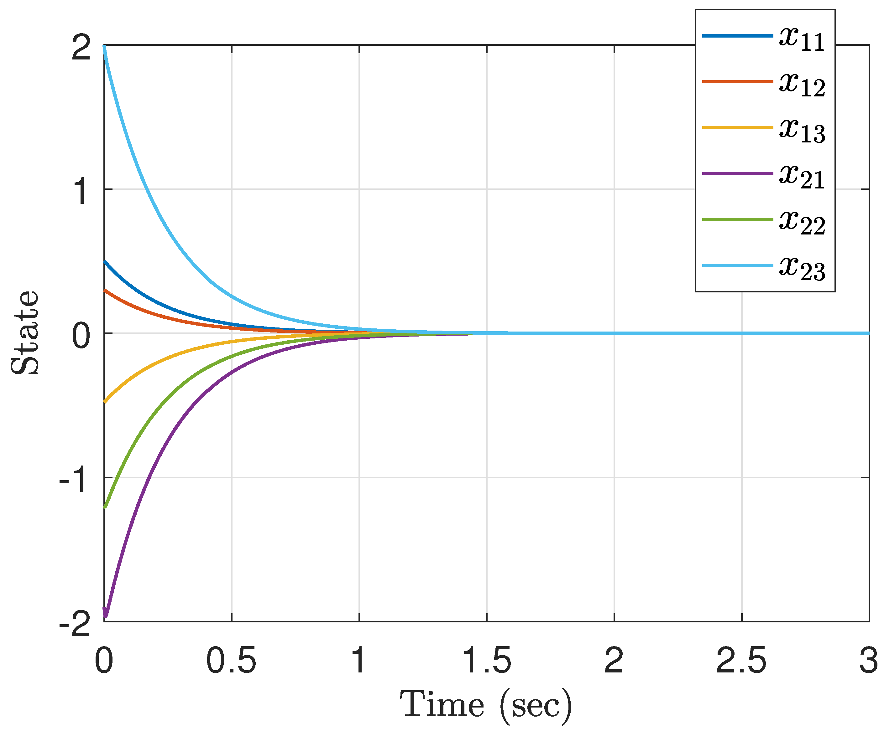
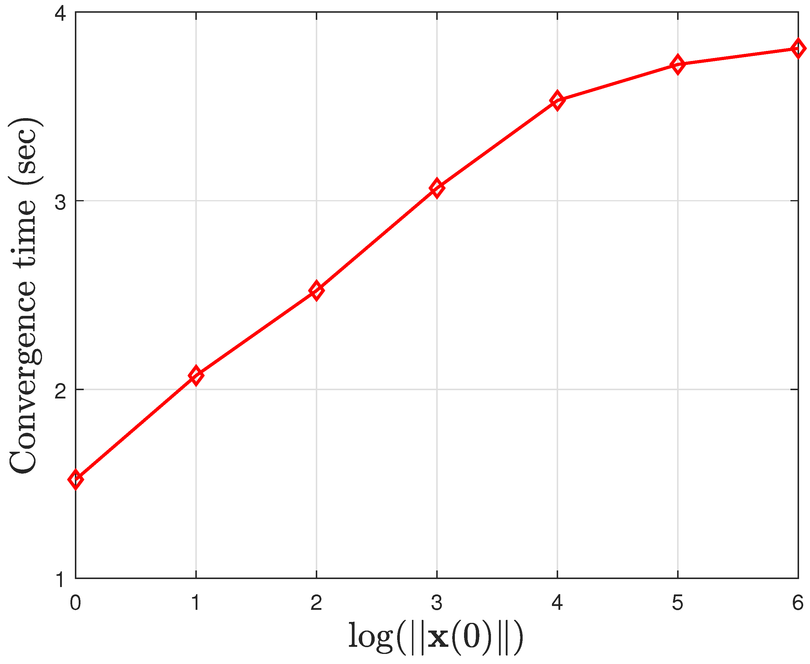
4. Simulation Studies

The proposed design approach is now applied to the attitude stabilization problem of a spacecraft. Consider the attitude control model of a spacecraft shown in [35,44], which has the same form as (1) with $n=m=3$. The system states of this model are the three Euler angles $(\varphi ,\theta ,\psi )$ and their derivatives $(\dot{\varphi },\dot{\theta },\dot{\psi })$, i.e., ${\mathbf{x}}_1={(x_{11},x_{12},x_{13})}^T={(\varphi ,\theta ,\psi )}^T$ and ${\mathbf{x}}_2={(x_{21},x_{22},x_{23})}^T={(\dot{\varphi },\dot{\theta },\dot{\psi })}^T$. Moreover, the drift term $\mathbf{f}(\mathbf{x},t)$ is time-invariant and $G(\mathbf{x},t)$ is a constant matrix [44]; thus, $\mathbf{f}(\mathbf{x},t)$ and $G(\mathbf{x},t)$ are briefly denoted by $\mathbf{f}\left(\mathbf{x}\right)={(f_1\left(\mathbf{x}\right),f_2\left(\mathbf{x}\right),f_3\left(\mathbf{x}\right))}^T$ and G, respectively, while having the following form [35]:

$$\begin{array}{cc}\hfill f_1\left(\mathbf{x}\right)& ={\omega }_0{x}_{23}c{x}_{13}c{x}_{12}-{\omega }_0{x}_{22}s{x}_{13}s{x}_{12}+\frac{I_y-I_z}{I_x}[x_{22}{x}_{23}+{\omega }_0{x}_{22}c{x}_{11}s{x}_{13}s{x}_{12}\hfill \\ \hfill & +{\omega }_0{x}_{22}c{x}_{13}s{x}_{11}+{\omega }_0{x}_{23}c{x}_{13}c{x}_{11}+\frac{1}{2}{\omega }_0^{2}s\left(2x_{13}\right)c^2{x}_{11}s{x}_{12}\hfill \\ \hfill & +\frac{1}{2}{w}_0^2{c}^2{x}_{13}s\left(2x_{11}\right)-{\omega }_0{x}_{23}s{x}_{13}s{x}_{12}s{x}_{11}-\frac{1}{2}{\omega }_0^2{s}^2{x}_{12}{s}^2{x}_{13}s\left(2x_{11}\right)\hfill \\ \hfill & -\frac{1}{2}{\omega }_0^{2}s\left(2x_{13}\right)s{x}_{12}{s}^2{x}_{11}-\frac{3}{2}{\omega }_0^2{c}^2{x}_{12}s\left(2x_{11}\right)]\hfill \end{array}$$

$$\begin{array}{cc}\hfill f_2\left(\mathbf{x}\right)& ={\omega }_0{x}_{23}s{x}_{13}c{x}_{11}+{\omega }_0{x}_{21}c{x}_{13}s{x}_{11}+{\omega }_0{x}_{23}c{x}_{13}s{x}_{12}s{x}_{11}\hfill \\ \hfill & +{\omega }_0{x}_{22}s{x}_{13}c{x}_{12}s{x}_{11}+{\omega }_0{x}_{21}s{x}_{13}s{x}_{12}c{x}_{11}+\frac{I_z-I_x}{I_y}[x_{21}{x}_{23}\hfill \\ \hfill & +{\omega }_0{x}_{21}c{x}_{11}s{x}_{13}s{x}_{12}+{\omega }_0{x}_{21}c{x}_{13}s{x}_{11}-{\omega }_0{x}_{23}s{x}_{13}c{x}_{12}\hfill \\ \hfill & -\frac{1}{2}{\omega }_0^{2}s\left(2x_{12}\right)s^2{x}_{13}c{x}_{11}-\frac{1}{2}{w}_0^{2}c{x}_{12}s{x}_{11}s\left(2x_{13}\right)+\frac{3}{2}{\omega }_0^{2}s\left(2x_{12}\right)c{x}_{11}]\hfill \end{array}$$

$$\begin{array}{cc}\hfill f_3\left(\mathbf{x}\right)& ={\omega }_0{x}_{21}s{x}_{11}s{x}_{13}s{x}_{12}-{\omega }_0{x}_{23}c{x}_{11}c{x}_{13}s{x}_{12}-{\omega }_0{x}_{22}c{x}_{11}s{x}_{13}c{x}_{12}\hfill \\ \hfill & +{\omega }_0{x}_{23}s{x}_{13}s{x}_{11}-{\omega }_0{x}_{21}c{x}_{13}c{x}_{11}+\frac{I_x-I_y}{I_z}[x_{21}{x}_{22}\hfill \\ \hfill & +{\omega }_0{x}_{21}c{x}_{13}c{x}_{11}-{\omega }_0{x}_{21}s{x}_{13}s{x}_{12}s{x}_{11}-{\omega }_0{x}_{22}s{x}_{13}c{x}_{12}\hfill \\ \hfill & -\frac{1}{2}{\omega }_0^{2}s\left(2x_{13}\right)c{x}_{12}c{x}_{11}+\frac{1}{2}{w}_0^2{s}^2{x}_{13}s{x}_{11}s\left(2x_{12}\right)-\frac{3}{2}{\omega }_0^{2}s\left(2x_{12}\right)s{x}_{11}]\hfill \end{array}$$

$$\begin{array}{cc}\hfill G=& \left(\begin{array}{ccc}0.67& 0.67& 0.67\\ 0.69& -0.69& -0.69\\ 0.28& 0.28& -0.28\end{array}\right).\hfill \end{array}$$

Here, $I_x=2000N·m·se{c}^2$, $I_y=400N·m·se{c}^2$, and $I_z=2000N·m·se{c}^2$ are the inertias of the coordinate axes, ${\omega }_0=1.0312\times {10}^{-3}$ rad/sec denotes the orbital rate, and $s(·)$ and $c(·)$ represent the sine and cosine functions, respectively. Additionally, we also assume that the attitude model suffers from the following discontinuous disturbances

$$\begin{array}{c}\hfill \mathbf{d}(\mathbf{x},t)=\left\{\begin{array}{cc}{(sin\left(t\right),cos\left(2t\right),sin\left(3t\right))}^T\hfill & \mathrm{if}t\le 0.4sec\hfill \\ 0.1{(cos\left(3t\right),sin\left(t\right),cos\left(2t\right))}^T\hfill & \mathrm{if}t>0.4sec\hfill \end{array}\right..\end{array}$$

For demonstration, the parameters ${\kappa }_1$ and ${\kappa }_2$ are selected as ${\kappa }_1=-2/15$ and ${\kappa }_2=2/15$, respectively. With these settings, the settling-time estimate is $T_{max}=35$ and the associated gain matrices ${\mathcal{L}}_1\left(\mathbf{x}\right)$, ${\mathcal{L}}_2\left(\mathbf{x}\right)$, and $\mathrm{\Phi }\left(\mathbf{x}\right)$ can be determined accordingly.

The simulation results shown in Figure 1 and Figure 2 are conducted for the initial state $\mathbf{x}\left(0\right)=(0.5,0.3,-0.48,-1.9,$${-1.2,2)}^T$. Clearly, Figure 1 shows that the finite-time stabilization task can be successfully performed by the corresponding control signals shown in Figure 2, where the abrupt changes in the control signals originate from the discontinuity of $\mathbf{d}(\mathbf{x},t)$ at $t=0.4$ s. It can be found that the settling-time (convergence time) of state trajectories is much less than $T_{max}=35$ (i.e., the settling-time estimate). This in turn reveals that the fixed-time stabilization can be achieved by the controller designed by Theorem 1. In addition, Figure 3 depicts the convergence times of the simulations conducted with different initial states from which one can observe that the correspondence between the convergence time and initial state, and obtain, moreover, the same conclusion (i.e., the success of the fixed-time stabilization). Notably, this example exhibits the merits and effectiveness of the proposed approach.

5. Conclusions

This paper has addressed the problem of fixed-time stabilization for a class of second-order (multivariable) nonlinear systems. A new design approach was developed by skillfully introducing extra manipulations in the feedback domination and delicately revamping the technique of adding a power integrator. Under the presented approach, a state feedback fixed-time stabilizing controller and a Lyapunov function for verifying fixed-time convergence can be organized explicitly. An example of the spacecraft attitude stabilization was also presented to demonstrate the effectiveness of our method.

References

1. Krstic, M.; Kanellakopoulos, I.; Kokotovic, P.V. Nonlinear and Adaptive Control Design; John Wiley: New York, NY, USA, 1995. [Google Scholar]
2. Isidori, A. Nonlinear Control Systems, 3rd ed.; Springer: New York, NY, USA, 1995. [Google Scholar]
3. Ding, S.; Mei, K.; Li, S. A new second-order sliding mode and its application to nonlinear constrained systems. IEEE Trans. Autom. Control. 2019, 64, 2545–2552. [Google Scholar] [CrossRef]
4. Wang, L.X. Stable adaptive fuzzy control of nonlinear systems. IEEE Trans. Fuzzy Syst. 1993, 1, 146–155. [Google Scholar] [CrossRef]
5. Xiang, Z.; Qiao, C.; Mahmoud, S. Finite-time analysis and H control for switched stochastic systems. J. Frankl. Inst. 2012, 349, 915–927. [Google Scholar] [CrossRef]
6. Ding, S.; Li, S.; Zheng, W.X. Nonsmooth stabilization of a class of nonlinear cascaded systems. Automatica 2012, 48, 2597–2606. [Google Scholar] [CrossRef]
7. Du, H.; Qian, C.; Li, S.; Chu, Z. Global sampled-data output feedback stabilization for a class of uncertain nonlinear systems. Automatica 2019, 99, 403–411. [Google Scholar] [CrossRef]
8. Cheng, Y.; Zhang, J.; Du, H.; Wen, G.; Lin, X. Global event-triggered output feedback stabilization of a class of nonlinear systems. IEEE Trans. Syst. Man Cybern. Syst. 2019, in press. [Google Scholar] [CrossRef]
9. Bhat, S.P.; Bernstein, D.S. Finite-time stability of continuous autonomous systems. SIAM J. Control. Optim. 2000, 38, 751–766. [Google Scholar] [CrossRef]
10. Moulay, E.; Perruquetti, W. Finite time stability conditions for non-autonomous continuous system. Int. J. Control. 2008, 81, 797–803. [Google Scholar] [CrossRef]
11. Liu, Y. Global finite-time stabilization via time-varying feedback for uncertain nonlinear systems. SIAM J. Control. Optim. 2014, 52, 1886–1913. [Google Scholar] [CrossRef]
12. Sun, Z.Y.; Xue, L.R.; Zhang, K. A new approach to finite-time adaptive stabilization of high-order uncertain nonlinear system. Automatica 2015, 58, 60–66. [Google Scholar] [CrossRef]
13. Fang, L.; Ma, L.; Ding, S.; Zhao, D. Finite-time stabilization for a class of high-order stochastic nonlinear systems with an output constraint. Appl. Math. Comput. 2019, 358, 63–79. [Google Scholar] [CrossRef]
14. Shen, Y.; Huang, Y. Global finite-time stabilisation for a class of nonlinear systems. Int. J. Syst. Sci. 2012, 43, 73–78. [Google Scholar] [CrossRef]
15. Huang, S.; Xiang, Z. Finite-time stabilisation of a class of switched nonlinear systems with state constraints. Int. J. Control. 2018, 91, 1300–1313. [Google Scholar] [CrossRef]
16. Chen, C.C.; Sun, Z.Y. A unified approach to finite-time stabilization of high-order nonlinear systems with an asymmetric output constraint. Automatica 2019, in press. [Google Scholar] [CrossRef]
17. Wu, D.; Du, H.; Wen, G.; Lü, J. Fixed-time synchronization control for a class of master-slave systems based on homogeneous method. IEEE Trans. Circuits Syst. II Express Briefs 2019, in press. [Google Scholar] [CrossRef]
18. Chen, C.C. A unified approach to finite-time stabilization of high-order nonlinear systems with and without an output constraint. Int. J. Robust Nonlinear Control. 2019, 29, 393–407. [Google Scholar] [CrossRef]
19. Zhai, J.; Song, Z.; Karimi, H.R. Global finite-time control for a class of switched nonlinear systems with different powers via output feedback. Int. J. Syst. Sci. 2018, 49, 2776–2783. [Google Scholar] [CrossRef]
20. Man, Z.; Paplinski, A.P.; Wu, H.R. A robust MIMO terminal sliding mode control scheme for rigid robotic manipulators. IEEE Trans. Autom. Control. 1994, 39, 2464–2496. [Google Scholar]
21. Feng, Y.; Yu, X.; Man, Z. Non-singular terminal sliding mode control of rigid manipulators. Automatica 2002, 38, 2159–2167. [Google Scholar] [CrossRef]
22. Xu, S.S.D.; Chen, C.C.; Wu, Z.L. Study of nonsingular fast terminal sliding-mode fault-tolerant control. IEEE Trans. Ind. Electron. 2015, 62, 3906–3913. [Google Scholar] [CrossRef]
23. Polyakov, A. Nonlinear feedback design for fixed-time stabilization of linear control systems. IEEE Trans. Autom. Control. 2012, 57, 2106–2110. [Google Scholar] [CrossRef] [Green Version]
24. Chen, C.C.; Sun, Z.Y. Fixed-time stabilisation for a class of high-order nonlinear systems. IET Control. Theory Appl. 2018, 12, 2578–2587. [Google Scholar] [CrossRef]
25. Cruz-Zavala, E.; Moreno, J.A.; Fridman, L.M. Uniform robust exact differentiator. IEEE Trans. Autom. Control. 2011, 56, 2727–2733. [Google Scholar] [CrossRef]
26. Gao, F.; Wu, Y.; Zhang, Z.; Liu, Y. Global fixed-time stabilization for a class of switched nonlinear systems with general powers and its application. Nonlinear Anal. Hybrid Syst. 2019, 31, 56–68. [Google Scholar] [CrossRef]
27. Basin, M.; Shtessel, Y.; Aldukali, F. Continuous finite- and fixed-time high-order regulators. J. Frankl. Inst. 2016, 353, 5001–5012. [Google Scholar] [CrossRef]
28. Zuo, Z. Nonsingular fixed-time consensus tracking for second-order multi-agent networks. Automatica 2015, 54, 305–309. [Google Scholar] [CrossRef]
29. Zuo, Z.; Han, Q.L.; Ning, B.; Ge, X.; Zhang, X.M. An overview of recent advances in fixed-time cooperative control of multiagent systems. IEEE Trans. Ind. Inf. 2018, 14, 2322–2334. [Google Scholar] [CrossRef]
30. Ni, J.; Liu, L.; Liu, C.; Hu, X.; Li, S. Fast fixed-time nonsingular terminal sliding mode control and its application to chaos suppression in power system. IEEE Trans. Circuits Syst. II Express Briefs 2017, 64, 151–155. [Google Scholar] [CrossRef]
31. Basin, M.; Panathula, C.B.; Shtessel, Y. Multivariable continuous fixed-time secondorder sliding mode control: design and convergence time estimation. IET Control. Theory Appl. 2017, 11, 1104–1111. [Google Scholar] [CrossRef]
32. Polyakov, A.; Efimov, D.; Perruquetti, W. Robust stabilization of MIMO systems in finite/fixed time. Int. J. Robust Nonlinear Control. 2016, 26, 69–90. [Google Scholar] [CrossRef] [Green Version]
33. Jiang, B.; Hu, Q.; Friswell, M.I. Fixed-time attitude control for rigid spacecraft with actuator saturation and faults. IEEE Trans. Control. Syst. Technol. 2016, 24, 1892–1898. [Google Scholar] [CrossRef]
34. Qian, C.; Lin, W. A continuous feedback approach to global strong stabilization of nonlinear systems. IEEE Trans. Autom. Control. 2001, 46, 1061–1079. [Google Scholar] [CrossRef]
35. Chen, C.C.; Xu, S.S.D.; Liang, Y.W. Study of nonlinear integral sliding mode fault-tolerant control. IEEE/ASME Trans. Mechatron. 2016, 21, 1160–1168. [Google Scholar] [CrossRef]
36. Xiao, B.; Yang, X.; Karimi, H.K.; Qiu, J. Asymptotic tracking control for a more representative class of uncertain nonlinear systems with mismatched uncertainties. IEEE Trans. Ind. Electron. 2019, in press. [Google Scholar] [CrossRef]
37. Pan, Y.; Li, X.; Yu, H. Efficient PID tracking control of robotic manipulators driven by compliant actuators. IEEE Trans. Control. Syst. Technol. 2019. [Google Scholar] [CrossRef]
38. Filippov, A.F. Differential Equations with Discontinuous Righthand Sides; Kluwer Academic Publishers: Dordrechts, The Netherlands, 1988. [Google Scholar]
39. Orlov, Y. Finite time stability and robust control synthesis of uncertain switched systems. SIAM J. Control. Optim. 2004, 43, 1253–1271. [Google Scholar] [CrossRef]
40. Chen, C.C.; Sun, Z.Y. A new approach to stabilisation of a class of nonlinear systems with an output constraint. Int. J. Control. 2019, in press. [Google Scholar] [CrossRef]
41. Hardy, G.; Littlewood, J.; Polya, G. Inequalities; Cambridge University Press: Cambridge, UK, 1988. [Google Scholar]
42. Royden, H.L.; Fitzpatrik, P.M. Real Analysis, 4th ed.; Pearson: Upper Saddle River, NJ, USA, 2010. [Google Scholar]
43. Bacciotti, A.; Rosier, L. Liapunov Functions and Stability in Control Theory, 2nd ed.; Springer: Berlin, Germany, 2005. [Google Scholar]
44. Chobotov, V.A. Spacecraft Attitude Dynamics and Control; Krieger: Malabare, FL, USA, 1991. [Google Scholar]
45. Zoriach, V.A. Mathematical Analysis II; Springer: Berlin, Germany, 2016. [Google Scholar]
Figure 1. State trajectories of the closed-loop system.
Applsci 10 00424 g001
Figure 2. Control signals of the closed-loop system.
Applsci 10 00424 g002
Figure 3. Convergence times for different initial states.
Applsci 10 00424 g003