Abstract
With the developing of high integrations in large scale systems, such as aircraft and other industrial systems, there are new challenges in safety analysis due to the complexity of the mission process and the more complicated coupling characteristic of multi-factors. Aiming at the evaluation of coupled factors as well as the risk of the mission, this paper proposes a combined technology based on the Decision Making Trial and Evaluation Laboratory (DEMATEL) model and the Bayesian network (BN). After identifying and classifying the risk factors from the perspectives of humans, machines, the environment, and management, the DEMATEL technique is adopted to assess their direct and/or indirect coupling relationships to determine the importance and causality of each factor; moreover, the relationship matrix in the DEMATEL model is used to generate the BN model, including its parameterization. The inverse reasoning theory is then implemented to derive the probability, and the risk of the coupled factors is evaluated by an assessment model integrating the probability and severity. Furthermore, the key risk factors are identified based on the risk radar diagram and the Pareto rule to support the preventive measurements. Finally, an application of the take-off process of aircraft is provided to demonstrate the proposed method.
1. Introduction
The risk evaluation of coupled factors throughout the system mission process has received increasing attention in recent years due to its effectiveness in preventing hazards and ensuring system safety, which offers a potential application in safety risk analysis. Safety analysis and risk assessment aim to eliminate and control various hazards through design activities and preventive measures, so as to prevent accidents that lead to casualties, equipment damage, and mission failures during the operation of the system [1,2]. With the development of science and technology, a series of analysis methods for evaluating system failures and risk events has been developed, especially in high-risk fields such as aerospace, chemical, nuclear, and other industrial fields. However, these methods have been found to be insufficient in a number of safety problems caused by the coupling characteristics in complex large scale systems.
The current safety analysis methods can be divided into single-factor and multi-factor analysis due to the differences in analysis objects [3], which have been extensively studied and have achieved good results. Specifically, failure mode and effects analysis (FMEA), functional hazard analysis (FHA), preliminary hazard analysis (PHA), and hazard and operability analysis (HAZOP) are effective methods for identifying and analyzing single failure modes or risk factors. For example, Soubiran et al. realized the safe guidance design of a train system by combining PHA and FMEA methods [4], Zhao et al. improved the risk assessment model based on fuzzy theory and the analytic hierarchy process (AHP), which provided a more accurate evaluation results [5,6], and Chudleigh [7] and Jagtman [8] applied the HAZOP method to medical diagnostic systems and road-safety measures, to identify not only hazards but also operational problems.
Moreover, with the development of the accident cause theory, a large number of methods for multi-factor safety analysis, such as fault tree analysis (FTA), Petri nets, Bayesian networks, etc., have also been invented. For example, Peeters et al. [9] combined FTA and FMEA in a recursive manner and applied it to an additive manufacturing system, so as to improve the efficiency of risk analysis. However, there exists in the method a defect whereby the bottom events in the fault tree model need to be independent. Gonçalves et al. [10] presented a safety assessment of unmanned aerial vehicles (UAVs) based on Petri nets, with the operation of the system represented by Petri nets to avoid undesired events.
A Bayesian network (BN) is a directed acyclic graph (DAG) composed of nodes and arcs, and its structure is very suitable for displaying important causal relationships among various factors, and provides a powerful framework for the research of complex coupling relationships [11,12]. The main advantage of a BN is to calculate the probability of occurrence of other uncertain nodes through an effective algorithm after determining any set of nodes [13]. Xiao et al. [14] established the structure of a BN through a simple questionnaire survey, and Constantinou et al. [15] proposed a BN modeling method based on a health assessment survey, which provided guidance for the management of survey data. In addition, Abimbola et al. [16] constructed a dynamic Bayesian network (DBN) by adding time variables, so as to carry out dynamic risk analysis for deep water drilling operations. However, the current BN modeling methods mainly have two weaknesses. The methods are effective in assessing potential risk factors, but with little consideration about the coupling relationships, which may reduce the completeness of these analyses. The methods also have a strong dependence on the experience of the analysts, which may lead to the inaccuracy and inconsistency of the models.
For the reason that current safety risk analysis technology is insufficient to solve the coupling problem among risk factors, scholars from various fields have implemented valuable explorations on qualitative coupling mechanism analysis, and applied them to the field of safety risk analysis. For example, Liou [17] proposed a hierarchical and structured safety assessment method, which solved the complex relationship among many risk factors in air transportation, Liu et al. [18] studied the coupling mechanism of safety risk in air traffic control and put forward a strategy of safety risk coupling management, Lin et al. [19] analyzed the original causes of aviation accidents and constructed a model of an aircraft safety management diagram based on coupling theory, and Wu et al. [20,21] studied the coupling mechanism between failures and proposed a phased-mission system analysis method considering common cause failures, using XML to realize automatic modeling and analysis. Moreover, many scholars use visual models and coupling coordination theory to establish multi-factor coupling mechanism models, which are widely used in the fields of coal mine production [22], waterway transportation, and highway transportation [23]. However, the above safety analysis methods mainly focused on a qualitative description and the study of coupling mechanisms, and lack the quantitative analyses and evaluations of coupling relationships.
One way to evaluate a coupling relationship is to adopt a reasonable mathematical model to assess the degree of mutual influence between factors, and there has been various models developed, such as structural equation modeling (SEM), interpretative structural modeling (ISM), N-K models, etc. Numerous studies have demonstrated that these methods are powerful and efficient. For example, Guo et al. [24] adopted the SEM model to analyze the causal relationship between risk factors in the coal mine safety, and the results provided guidance for practical risk assessment. Yang et al. [25] utilized the SEM model to discuss the relationship between various variables of business performance of an insurance company. Yin et al. [26] and Guan et al. [27] discovered the most direct and fundamental factors through application of an ISM model. Luo et al. [28] calculated the probability of multi-factor coupling by using an N-K model. However, the application of the above methods requires a large amount of historical and archived data, which may result in a limitation on the use of the methods in view of the potential lack of integrity and sample size of the data.
On the other hand, the Decision Making Trial and Evaluation Laboratory (DEMATEL) model, developed by the Battelle Memorial Institute [29], is a key technique in resolving problems associated with the coupling relationship. It was initially applied to investigate complex world problems, including racial issues, starvation, environmental protection, and energy consumption [30,31]. The DEMATEL model can transform sophisticated systems into precise causal relationships in structure, so that the quantified extent of direct and/or indirect causality among coupled risk factors can be evaluated using matrix operations and mathematical theories to help find the core problem [32,33].
This paper presents a combined technology based on the DEMATEL model and a Bayesian network, aiming at analyzing and evaluating the risk of factors considering the coupling relationship, so as to identify the key risk factors and high-risk regions. There are two benefits to using the proposed technology. Firstly, the structure diagram of the BN is established based on the direct-relation matrix; secondly, the conditional probability is calculated based on the direct–indirect matrix, and the parameterization of the Bayesian network is then completed. Inheriting the capability of the higher uncertainty reasoning of the Bayesian network, this combination of two models provides not only the basis for the Bayesian network based on the results of the DEMATEL model, but also an alternative approach of the assessment of coupled risk factors.
The remainder of the paper is organized as follows. Section 2 describes the hierarchical structure and the coupling evaluation methods of coupled risk factors. Section 3 expounds on the development and detailed steps of the proposed analysis method. Section 4 introduces an application of the take-off process of a carrier-based aircraft. Section 5 presents the conclusions.
2. Coupling Analysis of Risk Factors
2.1. Hierarchical Structure of Risk Factors
There are many risk factors that can result in accidents in a system, and they can be hierarchically divided for easy analysis and management. As the degree of refinement deepens, the number of risk factors at each level increases. When we classify the factors, a factor set that is too small will cause risk analysis inconvenience and difficulties, while a set that is too large will be more inaccurate, so it is effective to establish a management system of risk factors by classifying factors, so as to meet the practical necessities of risk analysis. Based on the fact that the failure of the mission process of a complex industrial system is usually caused by various factors, such as humans, machines, the environment, and management, the management system of risk factors can be divided into three levels to include the above four aspects. Specifically, the first level comprises four risk factors: human, machine, environment, and management factors. The second level is the further refinement of the first one; for instance, human factors can be divided further into profession skills, safety awareness, and physical and psychological status. The third level includes concrete risk factors determined by the analysis of the mission process, such as the various deviations obtained in the HAZOP analysis. Moreover, the third-level factors can be incorporated into the corresponding second-level factors through their characteristics analysis, so as to, considering their coupling relationships, quantify and analyze the safety and risk of the system with the second-level factors. The hierarchical relationship of risk factors is shown in Table 1.

Table 1.
The hierarchical relationship of risk factors.
2.2. Coupling Relationship Analysis of Risk Factors
There are inevitable interactions and/or couplings among various factors during the operation of a system, which can engender non-negligible effects on the safe operation of the system when a deviation occurs. Furthermore, these factors are generally attributed to one of four aspects, i.e. human, machine, environment, and management factors. Therefore, the coupling relationship can be divided into double-factor coupling and multi-factor coupling from these four aspects.
The couplings of double-factors and multi-factors, respectively, consider the direct and indirect coupling effects of two or more risk factors on the basis of the single-factor hazard analysis [3]. More precisely, the risk analysis of a single factor is a comprehensive quantitative assessment of the probability and severity of the factor [34], which takes the second-level factors as the objects, such as the evaluation of the impact of the professional skills of a human on the system risk.
The double-factor coupling involves two risk factors, and mainly focuses on the impacts of the occurrence of one factor on the other, namely the direct causal level between the two factors. For instance, the insufficient safety training may lead to the absence in the regular inspection of the machine, which may further increase the safety risk of the system.
The multi-factor coupling focuses on three or more risk factors, mainly taking the indirect causal effects of other risk factors into account on the basis of double-factor coupling. For instance, the insufficient safety training may lead to the lack of safe awareness of humans, which further results in the absence in the regular inspection of the machine.
2.3. Coupling Relationship Assessment Method of Risk Factors
The essence of the evaluation of the coupling relationship between risk factors is to use a unified measurement model to describe the degree of synergy within the factors, providing a direction for solving coupling problems in management, economics, and other fields [35,36]. The analytic hierarchy process (AHP) is a popular method for determining the contribution degree of each factor by establishing the hierarchical structure and the judgment matrix between the factors. This method has been widely used because of its simple operation and strong practicability, but it is difficult to solve the indirect influence between the factors. When the indirect effects are not negligible, the results obtained by the AHP may be out of line with the actual values.
Compared with the AHP method, DEMATEL technology is more comprehensive and effective in evaluating the coupling relationship of risk factors. DEMATEL technology also utilizes the matrix to evaluate the coupling relationship between factors, mainly including two matrices. One is the direct-relation matrix to assess the direct coupling relationship between factors, and the other is the direct–indirect matrix to represent the sum of the direct and/or indirect relationship between factors. Therefore, the use of DEMATEL technology in the assessment of coupled risk factors is conducive to systematically and accurately comprehending the total coupling relationships among factors, so as to provide reasonable and credible information for risk analysis.
3. An Integrated Method Based on the Decision Making Trial and Evaluation Laboratory (DEMATEL) Model and a Bayesian Network (BN)
3.1. The Main Process of the Method
Figure 1 describes the analysis process of the risk factors considering their coupling relationships. There are four main stages in the process. Firstly, the HAZOP method is adopted to identify hazards and operational problems during the missions of the system, in which the deviations are translated into the corresponding risk factors, namely the third-level factors shown in Table 1. The third-level factors can be incorporated into the corresponding second-level factors through characteristic analysis so that the classification diagram of risk factors can be obtained. Secondly, the DEMATEL model is applied to quantify the direct–indirect coupling relationship between risk factors, through which the importance–causality diagram is established to judge the importance and attribution degree according to the position of each factor. The structure and the parameterization of the Bayesian network (BN) are then accomplished based on the direct-relation matrix and the direct–indirect matrix in the DEMATEL model, respectively. Furthermore, the inverse reasoning theory of the BN is implemented to derive the probability of coupled risk factors, and the probability vector is obtained. Ultimately, the risk evaluation model, considering the probability and severity of coupled risk factors, is established, and can be used to construct a risk radar diagram. Moreover, the priority of risk factors is evaluated based on the Pareto rule. After a detailed analysis of high-risk regions and key factors, the preventive measurements can be proposed to control and reduce the risk level of the mission process.
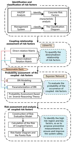
Figure 1.
The description of the proposed method.
3.2. The Identification and Classification of Risk Factors Based on Hazard and Operability Analysis (HAZOP)
The HAZOP analysis is a highly organized, structured, and organized technique to identify and analyze the hazards and operational problems in the system, in which the deviations can be regarded as “potential risk factors inconsistent with the design intention” [3]. Thus, when applying the HAZOP method to identify and classify the factors, the nodes are determined aiming at the mission process and the deviations are defined as the concrete risk factors , namely the third-level factors shown in Table 1. These factors are further incorporated into the corresponding second-level factors to support the following analysis. The improved HAZOP table is shown in Table 2, where a new column of “risk type” is added to the table to identify the second-level risk.
Table 2.
The improved hazard and operability analysis (HAZOP).
3.3. Coupling Relationship Assessment Based on the DEMATEL Model
DEMATEL technology is primarily applied to quantify the direct–indirect coupling relationship of risk factors, through which the importance–causality diagram can be established to analyze the importance and attribution degree according to the position of each factor [36]. Moreover, the DEMATEL model provides a reasonable basis for the Bayesian network, mainly reflected in the following two aspects. One is to establish the structure of the BN based on the direct-relation matrix, and the other is to parameterize the BN based on the conditional probability of factors calculated on the direct–indirect matrix. The specific steps of DEMATEL analysis are as follows [30,31,32,33,37].
1. Define the Evaluation Scale
The degree of causality among risk factors is defined as k levels, i.e., 0, 1, 2, …, k − 1, where 0 represents no causal relationship, and k-1 represents the strongest causal relationship.
2. Establish a Direct-Relation Matrix
The expert scoring method is used to evaluate the degree of direct causal relationship between two risk factors, and the direct-relation matrix M is then obtained by averaging the scores of each factor. If there are m kinds of risk factors, a matrix of will be determined, in which the element represents the degree of direct influence of the factor i on the occurrence of factor j. It is clear that the diagonal elements of the matrix are 0 because we focus on the relationship between different factors.
3. Normalize the Direct-Relation Matrix
According to the theory of matrix operation, the direct-relation matrix should be normalized to ensure the matrix convergence during the power series operation. In this paper, the sum of all matrix elements is used to normalize the matrix.
4. Calculate the Direct–Indirect Matrix
The direct–indirect matrix takes all the indirect effects among factors into account, and these indirect effects can be represented by the state transition process in the theory of absorbing a Markov chain matrix; moreover, the degree of the effect will decrease as the number of state transitions increases. During matrix operating based on the above theory, represents the direct-relation matrix, represents the secondary-relation matrix, indicating the causal effect of risk factor on considering the indirect effect of one risk factor, as shown in Figure 2a, represents the cubic-relation matrix, indicating that the causal effect of risk factor on considering the indirect effect of two risk factors, as shown in Figure 2b, and so on. thus represents the xth relation matrix.
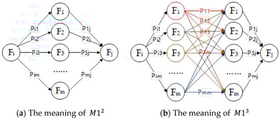
Figure 2.
The meanings of and .
The direct–indirect matrix can be calculated through a synthesis operation of the direct and indirect causal relationships according to Equation (2), and the element in can be used to evaluate the causal effect of risk factor on considering the indirect effects of all the risk factors.
5. Draw the Importance-Causality Diagram
The row sum of the matrix is defined as , which is called the influence degree, representing the synthetic effect of the factor on all other factors. The column sum is defined as , which is called the influenced degree, representing the synthetic effect of all other factors on the factor . The sum of and is called importance, representing the importance degree of factor i in the system safety risk, and the difference between and is called causality, representing the attributable causal level of factor i, with a positive value suggesting that the factor belongs to the cause category, and a negative value suggesting that the factor is in the result category.
Importance and causality are taken as the horizontal-axis and vertical-axis, respectively, and the factors are divided into four regions according to their positions. The meanings of these regions are shown in Figure 3.
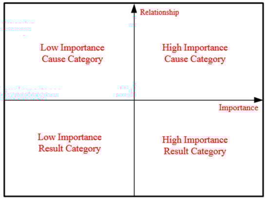
Figure 3.
The importance–causality diagram.
3.4. Probability Assessment of the Coupled Risk Factors Based on the BN
The Bayesian network is mainly applied to evaluate the probability of the occurrence of coupled risk factors, with the specific process as follows.
1. BN modeling Based on the Direct-Relation Matrix in the DEMATEL Model
Although a BN utilizes a directed graph, while DEMATEL technology uses a direct-relation matrix, they are both effective tools for describing the direct causal relationship between factors. The direct-relation matrix can be utilized to construct the initial causal diagram, in which the possible circulations can be eliminated to obtain the modified BN diagram.
A threshold value for the direct-relation matrix is determined based on expert judgment, and the elements that are greater than the threshold value in the direct-relation matrix can be converted as valid nodes and arcs in the initial causal diagram [12]. In view of the possible circulations in the initial causal diagram, it is necessary to identify and eliminate the circulations based on the following principles in order to transform it to a BN.
- (1)
- The BN should reflect not only the causal relationship between factors, but also the directions. There may be circulations in the initial causal diagram due to vague concepts of correlation and causality. For instance, there is a strong causal relation in , but with no relation in .
- (2)
- Since the BN mainly represents the direct causal relationship, there may be circulations in the initial causal diagram due to the indirect causality.
- (3)
- There may be circulations in the initial causal diagram because of time or other variables that exert an influence on the causal relationship between factors.
The above principles are adopted to check the bidirectional arc and closed loop arc in the initial causal diagram, so as to identify and eliminate the cycle arcs to obtain a Bayesian network diagram.
2. The Parameterization of BN
The diagrams of the Bayesian network are visual descriptions of the factorization of joint probability distributions [38], where nodes represent risk factors, and arcs represent probability dependencies between factors. For the reason that a diagram can depict the structure of a probability domain but cannot supply numerical characteristics, the conditional probability table (CPT) of each node needs to be established to parameterize the BN. When two nodes and are directly connected, such as , and are viewed as parent node and child node, respectively. When performing the risk assessment based on a BN, the obtained risk factors as well as a “risk” event are defined as nodes with two states of occurrence and non-occurrence. The prior probability of all nodes and the conditional probability under the combination of all of the states of these nodes and their parent nodes are input into the CPT to complete the parameterization. The calculation of the prior probability and conditional probability of each node is as follows.
According to the classification of risk factors in Section 3.2, each node in the Bayesian network is a set of multiple concrete risk factors. If the node contains risk factors , the probability of each factor is . The prior probability of node is defined as , and the formula is as follows on the assumption that the factors are independent of each other.
When the node is conditional on its parent node , the probability is defined as , representing the probability of the occurrence of node when the parent node occurs. Thus, the problem of calculating the conditional probability can be converted to evaluate the contribution of the parent node to the node . Based on the analysis in Section 3.3, the direct–indirect matrix obtained by the DEMATEL model can be used to quantitatively evaluate the degree of causal influence between factors. The column of node in the direct–indirect matrix indicates the causal effect of other nodes on node , with representing the causal effect of node on node . Therefore, the calculation of the contribution of the node to the node is as follows.
3. The Probability Assessment Based on the Inverse Reasoning Theory
The input of virtual evidence, one of the basic operations of the probability model, is to set a new state probability distribution for the unobservable variables in the model, so as to query the new posterior probability distribution of other variables. When conducting a risk assessment based on the BN, the BN is firstly structured and parameterized, and the inverse reasoning theory is then introduced to derive the posterior probability of other nodes (each risk factor) by setting the virtual evidence of the probability distribution of all states of the node “Risk,” which is regarded as the probability of occurrence of each risk factor considering the coupling relationship. The calculation formula is as follows.
3.5. Risk Assessment and Analysis of Coupled Risk Factors
3.5.1. Construction of a Risk Evaluation Model
Risk is a comprehensive means to quantify the effects of various factors in the process of transferring dangers to accidents [34], and system safety analysis based on risk has been widely applied to the mission process of complex industrial systems. Similar to the traditional quantification methods from two perspectives of risk, i.e., the probability of occurrence and the severity of consequence, the evaluation model considering the coupling relationship in this paper is also based on the probability and severity of the coupled risk factors, but these two perspectives are integrated into one value.
The risk index matrix is established by qualitative analysis of probability and consequence, in which probability and consequence are classified into m levels and h levels, respectively. Thus, the dimension of the matrix is , with the elements representing the risk values at the corresponding probability and severity levels. The improved Euclidean distance formula is introduced as the risk evaluation model, as shown in Equation (8), in which the parameters represent the probability, the severity, and the risk evaluation values in the risk index matrix, respectively. are the preference corrections, and can be calculated by fitting using the historical data of the parameters .
To evaluate the coupling effects between risk factors, the parameters in the above formula should be amended further to obtain Equation (9), in which the parameters represent the risk values, the probability, and the severity of the coupled risk factors, respectively.
3.5.2. Calculation of the Risk of Coupled Factors
The risk of coupled factors can be evaluated using Equation (9) after the probability and severity considering the coupling relationship are calculated. The probability of each risk factor can be obtained based on the results in Section 3.4. Therefore, the following mainly focuses on the assessment of severity of coupled risk factors.
It can be known from the above that the degree of severity is classified into h levels, where the first level indicates that the consequences of risk factors are extremely weak, and the hth level indicates the strongest consequence. We can define the range of value as being from 0 to n, so the interval length of each severity level is . The expert scoring method is used to evaluate the consequence degree of a single risk factor from 0 to n, and the initial severity vector is obtained after taking the average.
Furthermore, the coupling effects between risk factors are considered to amend the severity. The weight vector , obtained from the operation of and based on the DEMATEL model, can be used to modify the vector and acquire the final vector .
The risk of each factor considering the coupling relationship can be calculated by substituting and into Equation (9).
3.5.3. Risk Analysis Based on the Risk Radar Diagram and Pareto Rule
The calculated risk values can be used to establish a risk radar diagram, which is divided into five regions based on risk levels, i.e. highest risk, high risk, medium risk, low risk, and lowest risk. According to the Pareto rule [39,40], it can be concluded that 80% of the accidents are originated from 20% of the hazards. Therefore, the risk considering the coupling effect are sorted in descending order, in which the top 20% are regarded as the key risk factors. Aimed at the high risk region and key risk factors, the causal relationship was further researched to propose preventive measurements, so as to reduce the risk level and improve system safety.
4. Application and Discussion
The proposed method was applied to the ski-jump take-off process of a carrier-based aircraft for illustration and validation purposes.
4.1. HAZOP Analysis
The take-off process can be divided into four mission stages, namely, pre-take-off preparation, horizontal acceleration running, ramp acceleration running, and aerial crawling [41], which includes 21 risk factors according to analysis. The classification diagram of risk factors and the analysis of HAZOP, as shown in Figure 4 and Table A1, respectively, are obtained based on the method proposed in Section 3.2.
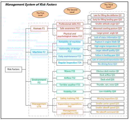
Figure 4.
The classification of risk factors.
4.2. Assessment of the Coupling Relationship Based on the DEMATEL Model
1. Establishment of the Evaluation Scale and the Direct-Relation Matrix
The evaluation scale established for the degree of causal relationship of risk factors is defined as 5 levels, i.e. 0, 1, 2, 3, and 4, where 0 represents no causality and 4 represents strongest causality. There are 14 kinds of risk factors based on the classification of 21 risk factors, and the degree of direct causal relationship will, based on expert judgment, be evaluated through pair-wise comparison, and the direct-relation matrix will be obtained after averaging.
2. Normalization of the Direct-Relation Matrix
The normalization of the direct-relation matrix is based on the formula 14, with the results shown in Table 3.
Table 3.
The results of the matrix.
3. Calculation of the Direct–Indirect Matrix
The calculation of the direct-indirect matrix is based on the formula 2, with the results shown in Table 4.
Table 4.
The results of the matrix.
4. Construction of the Importance–Causality Diagram
The construction of the importance–causality diagram is based on the calculations of the matrix M2, as shown in Table 5.
Table 5.
The calculations of the matrix.
The initial conclusions that can be drawn from Figure 5 are as follows:
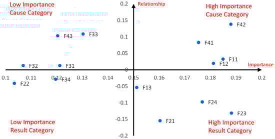
Figure 5.
The importance–causality diagram.
- High importance, cause category: , , , and belong to the cause category, which have a great impact on other risk factors and are less susceptible, but vary in the degree of relationship, with a strong relation on and and a weak relation on and . All of them are important factors in the mission.
- High importance, result category: and are more important than and throughout the mission, all of which belong to the result category, showing that the factors are vulnerable to other factors.
- Low importance, cause category: , , and belong to the cause category with a low value of and , which indicates less impact on other factors. The above factors are less important throughout the mission.
- Low importance, result category: and belong to the result category with a low value, which indicates less causality and less importance throughout the mission.
4.3. Probability Assessment of the Coupled Risk Factors Based on the BN
1. BN Modeling Based on the Direct-Relation Matrix in the DEMATEL Model
The direct-relation matrix in the DEMATEL model can be utilized to construct the Bayesian network, in which the numerical relationship in the matrix can be transformed into the structural relationship of the network because of the arcs in the BN representing the direct causal relationship. The possible circulations can be eliminated to obtain a modified BN diagram. In order to reduce the analysis work, a threshold of 2.5 is determined based on expert experience. The relationship of matrix elements above the threshold is regarded as a valid arc in the Bayesian network, so as to obtain the initial causal diagram. Based on the three principles described in Section 3.4, the initial casual diagram is checked and revised to eliminate the possible circulations to obtain the modified BN diagram, as shown in Figure 6.
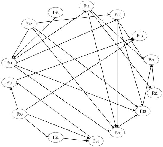
Figure 6.
The structure of the Bayesian network (BN).
2. The Parameterization of BN
The prior probability of each node is calculated according to Equation (4) based on the classification diagram of the risk factors obtained in Section 4.1. The results are shown in Table 6.
Table 6.
The results of the prior probability.
The conditional probability of each node with its parent node is calculated according to Equation (5) based on the direct–indirect matrix obtained by the DEMATEL model, and the results are shown in Table 7.
Table 7.
The results of the conditional probability.
3. The Probability Assessment Based on the Inverse Reasoning Theory
Based on the results of Table 6 and Table 7, the parameterization of the Bayesian network is completed. Moreover, virtual evidence is set for the node “Risk” to define the probability distribution of “occurrence” and “non-occurrence.” As a result, the probability of occurrence of other risk factors considering the coupling relationship is obtained, as shown in Figure 7.
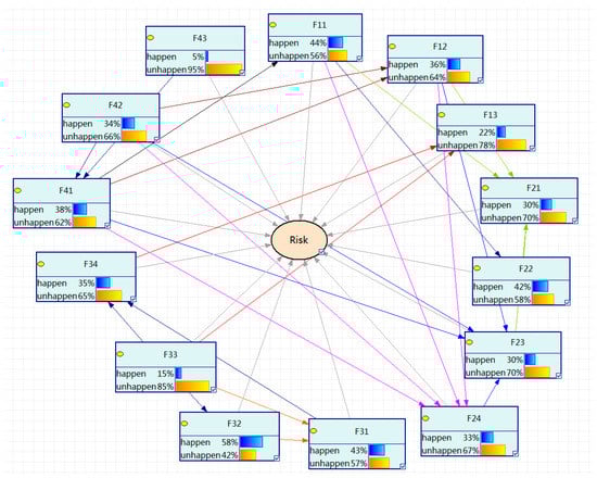
Figure 7.
The probabilistic inference diagram based on the BN.
4.4. Risk Assessment of the Coupled Risk Factors
4.4.1. The Probability of the Occurrence of Coupled Risk Factors
The probability of occurrence of coupled factors can be obtained based on the results in Figure 7, as shown in Table 8.
Table 8.
The probability of the occurrence of coupled factors.
4.4.2. The Severity of Coupled Risk Factors
The degree of severity is classified into five levels, where the range of value is from 0 to 10, and the interval length of each severity level is 2. The first level indicates that the consequences of risk factors are extremely weak, and the fifth level indicates the strongest consequence. The expert scoring method is used to obtain the initial vector , based on which the final vector is further acquired using the method proposed in Section 3.5, with the results shown in Table 9.
Table 9.
The calculation of the severity.
4.4.3. Risk Calculation of Coupled Risk Factors
The probability and consequence are classified into four levels and five levels, respectively, and the risk index matrix is established based on the historical risk values of all their state combinations; for instance, the historical risk is 19 when both levels are the highest [42]. Moreover, Equation (9) is fitted based on the method in Section 3.5 to determine the preference corrections . The amended risk evaluation model is shown in Equation (15).
The risk of each factor considering the coupling relationship can be calculated by introducing and to Equation (15), with the result shown in Table 10.
Table 10.
The risk of the coupled risk factors.
Some conclusions can be drawn from Figure 8:
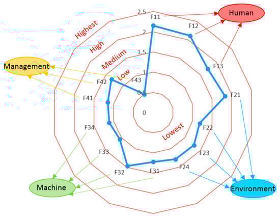
Figure 8.
The risk radar diagram.
- The top 20% of factors belong to the key risk factors according to the Pareto rule, so the risk factors have a higher risk level, which needs to be further analyzed to propose the preventive measurements.
- It can be concluded that the factors belong to the medium risk region, and the risk level of the factor is the lowest.
- According to the location distribution of risk factors in each category, the average risk level of human factors is the highest.
Based on the above analysis, it can be concluded that both and occupy high importance throughout the mission and belong to the cause category. They have a great impact on other risk factors and are less susceptible. Moreover, and , respectively, have the greatest impact on and . Therefore, the essence of reducing the risk level of human factors is to reduce the risk level of management factors. It is necessary to further strengthen the safety training and safety supervision system in order to enhance professional skills and safety awareness, so as to ensure the safety of the mission process of the system.
5. Conclusions
Aiming at the insufficiency of traditional safety risk analysis technology to solve the coupling problems between risk factors, this study proposes combined technology based on the DEMATEL model and the Bayesian network, aiming to analyze and evaluate the risk of factors considering the coupling of multi-factors in the mission process of complex industrial systems. The method can be summarized as the following four steps. Firstly, the risk factors are identified by the HAZOP method and classified according to the hierarchical structure. Secondly, the DEMATEL model is applied to quantify the direct–indirect coupling relationship between risk factors, through which the importance and attribution degree of each factor are acquired. The structure and parameterization of the Bayesian network are then accomplished to derive the probability of the coupled factors based on the results of the DEMATEL model. Ultimately, the risks of the coupled factors are calculated according to the established risk evaluation model. Furthermore, the key risk factors and the high-risk region are identified through the Pareto rule and risk radar diagram. Considering the take-off process of a shipboard aircraft as a case, the results indicate that (professional skills) and (safety awareness) occupy high importance throughout the mission, and the average risk level of the human factors is the highest, which provides a theoretical basis for putting forward preventive measures, so as to ensure and improve system safety. Compared with the current technologies, the method proposed in this paper mainly displays the advantages of the two aspects. Firstly, the construction and parameterization of the BN by adopting the DEMATEL model not only improve the analysis efficiency but also reduce the skill requirement for analysts. At the same time, it provides a feasible approach for the evaluation of the risk of coupled factors, which is the core judgment criterion for identifying key risk factors and of significance to ensure system safety.
Author Contributions
J.J. and T.Z. prepared the conception and the formal description of the proposed solution; they both performed the literature review; Y.Y. studied the case; M.W. and J.J. implemented the proposed solution and wrote the paper. All authors have read and agreed to the published version of the manuscript.
Funding
This research received no external funding.
Conflicts of Interest
The authors declare that there is no conflict of interest.
Appendix A
Table A1.
The improved HAZOP analysis (in part).
Table A1.
The improved HAZOP analysis (in part).
| Code | Event | Guidewords | Deviation | Risk Type | Cause of Deviation | Hazard Effect | Measures |
|---|---|---|---|---|---|---|---|
| pre-take-off preparation | omission | Missing inspections | The negligence of ground crew | Potential hazards may occur during take-off | Strength safety training and inspection | ||
| deficiency | Lack of status information | The failure in the display equipment or the power input | Pilots can’t judge the right position and status. | Change equipment regularly and check power supply | |||
| late | Late for lifting the deflector | The incorrect operation of the pilots | High temperature flame results in the damage of the deck. | Set up emergency equipment |
References
- An Institution of Civil Engineers. Risk Analysis and Management for Projects (RAMP); ICE Publishing: London, UK, 2009. [Google Scholar]
- Lorenc, A.; Kuźnar, M. An Intelligent System to Predict Risk and Costs of Cargo Thefts in Road Transport. Int. J. Eng. Technol. Innov. 2018, 8, 284–293. [Google Scholar]
- Wei, M.W.; Jiao, J.; Zhao, T.D. Coupling Multi-factor Hazard Analysis Based on HAZOP and DEMATEL. In Proceedings of the 66th Annual Reliability and Maintainability Symposium (RAMS 2020), Palm Springs, CA, USA, 27–30 January 2020. Charlie Plotkin. (accepted). [Google Scholar]
- Soubrian, E.; Guenab, F.; Canila, D. Ensuring Dependability and Performance for CPS Design: Application to a Signaling System. In Cyber-Physical System; Rawat, D.B., Jeschke, S., Brecher, C., Eds.; Academic Press: Boston, MA, USA, 2017. [Google Scholar]
- Zhao, Y.; Jiao, J.; Zhao, T.D. Risk Assessment Method Based on Fuzzy Logic. J. Syst. Eng. Electron. 2015, 37, 1025–1031. [Google Scholar]
- Zhao, Y.; Jiao, J.; Zhao, T.D. A Synthetic Risk Assessment Model Based On AHP. In Proceedings of the 60th Annual Reliability and Maintainability Symposium (RAMS 2014), Colorado Springs, CO, USA, 27–30 January 2014. [Google Scholar]
- Chudleigh, M.F. Hazard analysis of a computer based medical diagnostic system. Comput. Methods Programs Biomed. 1994, 44, 45–54. [Google Scholar] [CrossRef]
- Jagtman, H.M.; Hale, A.R.; Heijer, T. A support tool for identifying evaluation issues of road safety measures. Reliab. Eng. Syst. Saf. 2005, 90, 206–216. [Google Scholar] [CrossRef]
- Peeters, J.F.W.; Basten, R.J.I.; Tinga, T. Improving failure analysis efficiency by combining FTA and FMEA in a recursive manner. Reliab. Eng. Syst. Saf. 2018, 172, 36–44. [Google Scholar] [CrossRef]
- Goncalves, P.; Sobral, J.; Ferreira, L.A. Unmanned aerial vehicle safety assessment modelling through Petri Nets. Reliab. Eng. Syst. Saf. 2017, 167, 383–393. [Google Scholar] [CrossRef]
- Kaya, R.; Yet, B. Building Bayesian networks based on DEMATEL for multiple criteria decision problems: A supplier selection case study. Expert Syst. Appl. 2019, 134, 234–248. [Google Scholar] [CrossRef]
- Fenton, N.E.; Neil, M.; Caballero, J.G. Using ranked nodes to model qualitative judgements in Bayesian Networks. IEEE Trans. Knowl. Date Eng. 2007, 19, 1420–1432. [Google Scholar] [CrossRef]
- Lauritzen, S.L.; Spiegelhalter, D.J. Local Computations with Probabilities on Graphical Structures and Their Application to Expert Systems. J. R. Stat. Soc. Ser. B-Methodol. 1988, 2, 157–224. [Google Scholar] [CrossRef]
- Hu, X.X.; Wang, H.; Wang, S. Using Expert’s Knowledge to Build Bayesian Networks. In Proceedings of the 2007 International Conference on Computational Intelligence and Security Workshops (CISW 2007), Harbin, China, 15–19 December 2007; pp. 220–223. [Google Scholar]
- Constantinou, A.C.; Fenton, N.; Marsh, W. From complex questionnaire and interviewing data to intelligent Bayesian network models for medical decision support. Artif. Intell. Med. 2016, 67, 75–93. [Google Scholar] [CrossRef]
- Abimbola, M.; Khan, F.; Khakzard, N. Dynamic safety risk analysis of offshore drilling. J. Loss Prev. Process. Ind. 2014, 30, 74–85. [Google Scholar] [CrossRef]
- Liou, J.H.; Tzeng, G.H.; Chang, H.C. Airline safety measurement using a hybrid model. J. Air Transp. Manag. 2007, 13, 243–249. [Google Scholar] [CrossRef]
- Liu, T.Q.; Luo, F. Analysis on Constitution and Coupling of Air Traffic Security Risk. J. Wut (Inf. Manag. Eng.) 2012, 34, 93–97. [Google Scholar]
- Lin, J.H.; Li, K.W.; Zhang, B. Inherent safety management of aviation equipment based on risk coupling theory. J. Saf. Sci. Technol. 2011, 7, 75–79. [Google Scholar]
- Wu, H.; Jiao, J.; Zhao, T.D. A reliability modeling and analysis method for PMS considering common cause failure. J. Beijing Univ. Aeronaut. Astronaut. 2018, 44, 197–203. [Google Scholar]
- Wu, H.; Zhao, T.D.; Jiao, J. XML-Based Modeling Method of Phased-mission Systems Subject to Probabilistic Common Cause Failures. J. Intell. Fuzzy Syst. 2019, 36, 871–884. [Google Scholar] [CrossRef]
- Liu, Q.L.; Li, X.C.; Wang, L. Analysis and Management of Risk Factors Coupling in Coal Mine Accidents. Stat. Inf. Forum 2015, 30, 82–87. [Google Scholar]
- Liu, D.L.; Xu, H.J.; Zhang, J.X. Quantitative Risk Evaluation Methods for Multi-factor Coupling Complex Flight Situations. J. Aeronaut. Astronaut. 2012, 34, 509–516. [Google Scholar]
- Guo, K. Assessment of Coal Mine Safety Influencing Factors Based on Structural Equation Model. J. Coal Mine Saf. 2012, 7, 217–219. [Google Scholar]
- Yang, S.D.; He, J.M. Key influence factors for insurance company performance based on SEM. J. Southeast Univ. 2010, 12, 48–51. [Google Scholar]
- Yin, H.Y.; Xu, L.Q.; Quan, X.F. Research on Influencing Factors of Road Networks Vulnerability Based on Interpretive Structural Model. J. Soft Sci. 2010, 20, 122–126. [Google Scholar]
- Guan, W.J.; He, G.; Chen, Q.H. Analysis of Major Influencing Factors of Coal Mine Safety Based on ISM. J. Stat. Decis. 2010, 19, 178–179. [Google Scholar]
- Luo, F.; Liu, T.Q. Analysis of Coupled Risk of Air Traffic Safety Based on N-K Model. J. Wuhan Univ. Technol. 2011, 33, 267–270. [Google Scholar]
- Fontela, R.; Gabus, A. The DEMATEL Observer; DEMATEL 1976 Report; Battelle Geneva Research Center: Switzerland, Geneva, 1976. [Google Scholar]
- Hsin, H.Y.; Lee, Y.C. BPNN and DEMATEL to modify importance-performance analysis model—A study of the computer industry. Expert Syst. Appl. 2009, 36, 9969–9979. [Google Scholar]
- Lee, Y.C.; Li, M.L.; Yen, T.M. Analysis of adopting an integrated decision making trial and evaluation laboratory on a technology acceptance model. Expert Syst. Appl. 2010, 37, 1745–1754. [Google Scholar] [CrossRef]
- Luthra, S.; Govindan, K.; Kharb, R.K. Evaluating the enablers in solar power developments in the current scenario using fuzzy DEMATE: An Indian perspective. Renew. Sustain. Energy Rev. 2016, 63, 379–397. [Google Scholar] [CrossRef]
- Strantzali, E.; Aravossis, K. Decision making in renewable energy investments: A review. Renew. Sustain. Energy Rev. 2016, 55, 8885–8898. [Google Scholar] [CrossRef]
- Yong-sik, H.; Taekshin, E.; Sooeum, T. Inundation Risk Assessment of Underground Space Using Consequence-Probability Matrix. Appl. Sci. 2019, 9, 1196–1207. [Google Scholar]
- Wang, W.Z.; Zhang, G.B.; Lu, M.Y. Quantitative and analysis on critical risk factors of processing workshop based on multiple-factor coupling. J. Saf. Sci. Technol. 2015, 9, 158–164. [Google Scholar]
- Zhang, H.X.; Fu, Y.T.; Chen, M. Bi-Level Planning Model of Charging Stations Considering the Coupling Relationship between Charging Stations and Travel Route. Appl. Sci. 2018, 8, 1130. [Google Scholar] [CrossRef]
- Chen, K.H.; Yien, J.M.; Chiang, C.H.; Tsai, P.C.; Tsai, F.S. Identifying Key Sources of City Air Quality: A Hybrid MCDM Model and Improvement Strategies. Appl. Sci. 2019, 9, 1414. [Google Scholar] [CrossRef]
- Paul, J.H.; Mohsen, M.S.; Byron, D.E. Bayesian Inference of Vocal Fold Material Properties from Glottal Area Waveforms Using a 2D Finite Element Model. Appl. Sci. 2019, 9, 2735–2741. [Google Scholar]
- Tsai, S.B.; Xue, Y.Z. Models for forecasting growth trends in renewable energy. Renew. Sustain. Energy Rev. 2017, 77, 1069–1078. [Google Scholar] [CrossRef]
- Jure, M.; Janez, K.; Tomaz, B. Methodology for Searching Representative Elements. Appl. Sci. 2019, 9, 3482–3497. [Google Scholar]
- Li, L.W. Researcher on Flight Control and Visual Simulation for Ski-Jump Take-Off of Carrier-Based Aircraft. Master’s Thesis, Master of Engineering, Nanjing University of Aeronautics and Astronautics, Nanjing, China, 2016. [Google Scholar]
- Ni, H.H.; Chen, A.; Chen, N. Some extensions on risk matrix approach. Saf. Sci. 2010, 48, 1269–1278. [Google Scholar] [CrossRef]
© 2019 by the authors. Licensee MDPI, Basel, Switzerland. This article is an open access article distributed under the terms and conditions of the Creative Commons Attribution (CC BY) license (http://creativecommons.org/licenses/by/4.0/).