Development of a Pull Production Control Method for ETO Companies and Simulation for the Metallurgical Industry

Abstract

At the moment, many engineer-to-order manufacturers are under pressure, the overcapacity in many sectors erodes prices and many companies, especially in Europe have gone into recent years in bankruptcy. Due to the increasing competition as well as the new customer requirements, the internal processes of an ETO company play an essential role in order to achieve a unique selling proposition (USP). Therefore this paper exposes how the production planning and control of an engineer-to-order manufacturer can be designed in order to increase its OTD (order-to-delivery) rate as well as decrease the WIP (work-in-progress) and the production lead times. To prove the optimized planning logic, it was applied in a simulation case study and based on the results; the conclusions about its potential are derived.

1. Introduction

Markets for engineer-to-order (ETO) manufacturers that were stable in the past are now dynamic and uncertain in which prices have reduced over the last decades [1] (p. 43). At the moment, many ETO manufacturers, such as companies in the metallurgical sector, working for specific needs and end-segments such as the steel industry, are under pressure; the current overcapacity is destroying prices and profitability [2] (p. 2) and many producers have closed facilities, have made layoffs and have gone in bankruptcy in recent years [3] (pp. 1–2). As an example by the end of 2015, U.S. steel producers were utilizing less than 65% of their capacity, and were forced to lay off 12,000 employees in this year [3] (p. 1). In 2007–2011 capacity utilization was about 80% and supply and demand was in a balanced state, but since 2012 the overcapacity challenge was becoming obvious, with 74.8% in 2014 [4] (p. 62), less than 70% in 2015 [3] (p. 5) and with a recovery in 2018 due to a reduction of capacity since 2015 with 75.7% capacity utilization with 2233.7 million tons of capacity available [5] and 1690.1 of produced crude steel [6] (p. 2). The overcapacity created was driven by new investment from old market leaders as well as new emerging market companies in the last decades like in China, which now has two-thirds of world steel overcapacity [3] (p. 1).

On the other hand, in respond to that, ETO companies are continuously seeking for ways or methods how to reduce costs and lead times as well as increasing their external flexibility [1] (p. 43). In the literature there is limited research related to supply chain management in the low-volume engineer to order (ETO) sector, in contrast to the extensive literature on the high-volume sector, particularly automotive and electronics [7] (p. 179). The limited research that has been undertaken in the low volume ETO sector has focused on production control, information systems, manufacturing systems and the co-ordination of marketing and manufacturing [1] (p. 44).

In this global market situation, current producers need to work on their technological and organizational advantage. On the one side, the steel industry has a low frequency of innovation compared to other industries with process technologies have been used for decades [8] (p. 8). Until the recession in 1973, advanced countries such as US, Japan and European countries were increasing their steel production [8] (p. 9). Due to the recession, steel demand decreased and US and Japanese steel firms were forced to export their technology [8] (p. 10). Therefore, the first potential unique selling proposition (USP), the technological advantage, hardly exists anymore for US, Japanese, or European countries, as many companies worldwide have access and have invested in new equipment in recent decades and years, mainly in developing countries [9] (pp. 2–3) such as Korea, Taiwan, Brazil, and China [8] (p. 10).

For ETO companies, the question arises of what options remain to improve their competitive situation and to shape a long-term and profitable business model. In addition, additional cost savings programs will not be enough to achieve sustainable returns. For this reason, ETO producers need to be focus on the second potential USP, the internal process optimization, such as digitization and optimization of business processes enabling a better service level to end-customers.

1.1. Research Questions and Goals

On the basis of the previous paragraphs, this paper aims to provide a methodology for the improvement of internal processes in regard to production planning and control by optimizing internal parameters, work-in-progress (WIP), and production lead times, as well as end-customer service level, and order-to-delivery (OTD). The final goal of this optimization would be to increase the company’s competitiveness securing its long-term existence. Based on these objectives the following research questions can be declared:

• Which are current challenges of ETO manufacturers?
• Which is the current common production planning strategy being used in ETO industries?
• How do other production planning strategies can be applied to the ETO sector?
• What is the potential benefit of this change?
• In order to achieve these goals, this paper presents the following structure:
  • Introduction: definition of challenge, objectives, and simulation.
  • Literature review of:

    ○

    Engineer-to-order typology and characteristics;

    ○

    Organizational model for the order management process;

    ○

    Production planning and control: push versus pull;

    ○

    Capacity planning and maintenance;

    ○

    Theory of constraints (TOC) and drum-buffer-rope (DBR);

    ○

    Agent-based simulation.

  • Typical initial situation and development of pull production control for ETO manufacturers.
  • Applying the model for production control to the metallurgical industry through simulation.
  • Simulation results and implementation.
  • Conclusions.

The main expected outcome of the research paper is that a pull control approach using drum-buffer-rope (DBR) approach will lead to an improvement of OTD and to a reduction of lead times and WIP stocks.

1.2. Methodology Used

The research methodology for an ETO company consists of the steps shown in Figure 1:

Based on the previously described methodology two different models are simulated, a classical push production control model versus a pull production control. The main objectives are: to generate knowledge of the supply chain, development and validation of improvements using what would happen if of analysis and quantification of the benefits of decision support at the level of strategic decision making [10] (p. 4). One recent modeling method is agent-based simulation and it has no standard language. The structure of an agent based model is created using graphical editors depending on the software. The behavior of agents is specified in many different ways. Frequently, the agent has a notion of state, and its actions and reactions depend on its state [11] (p. 14). For the research work AnyLogic was used and the models presented production orders as agents with their own characteristics. As a consequence the research was qualitative in the conceptualization and quantitative for the simulation models and data used. In Figure 2 it can be shown the steps followed to perform the simulation of the two models:

2. Theoretical Background as the Basis for Model Development

2.1. Engineer-To-Order Typology and Characteristics

Based on the literature six different supply chain typologies can be defined to describe the range of possible operations: engineer-to-order (ETO), buy-to-order (BTO), make-to-order (MTO), assemble-to-order (ATO), make-to-stock (MTS), and ship-to-stock (STS). The ETO supply chain is described as a supply chain where the customer order decoupling point is located at the design stage, so each customer order influenced the design phase of a product [12] (p. 741).

The characteristics of the manufacturers with ETO are customized and high-value added products, in low volume with deep and complex product structure in order to meet specific customer requirements [1,7] (p. 43, p. 179). It is primarily associated with large, complex project environments in sectors such as construction and capital goods. However, while the term ETO is used, in the literature exists confusion about the appropriate strategies and there is no major systematic literature reviews or syntheses of knowledge relating to the ETO supply chain type [12] (p. 741).

2.2. Competitiveness

The competitive advantage of ETO companies is based on the fulfillment of individual customer requirements [13] (p. 16). This approach demands a high flexibility of the manufacturing process [14] (p. 1). The success factor is the capability to deliver the specific order in time [15] (p. 384). As a consequence, a short lead time and effective synchronization of the production management processes are key [14] (pp. 1–2) to gain competitiveness.

Between innovation and competitive advantage, there is a complex and multidimensional relationship [16,17], in which sustainability plays a primary role. Therefore, the innovation must be characterized by sustainability [18] (p. 8).

As an example, the competitiveness of steel production is based on a set of internal comparative advantages such as labor costs, consistent economy and foreign trade policy, long-term work experience, energy prices, or highly efficient work organization [19] (p. 122). These indicators provide us how these factors differ and how they affect the international competitiveness of steel products [19] (p. 122). Based on that, the EU is losing its competitiveness in those market segments where it is not possible to apply other competitive advantages such us: innovation, know-how, or scientific and research outputs for commercial purposes [19] (p. 120).

2.3. Organizational Model for the ETO’s Order Management Process

There are three stages of interaction between ETO companies and their customers. The first is marketing [7] (p. 188). The second stage is tendering that involves the preliminary development of the conceptual design and the definition of major components and systems. A technical specification, delivery schedule, price, and commercial terms are agreed. Of costs 75–80% are committed at this stage. The third stage takes place after a contract has been awarded and includes non-physical processes, such as design and planning, and physical processes associated with manufacturing, assembly and commissioning. Supply chain management in ETO companies involves the co-ordination of internal processes across these three stages [7] (p. 188)

ETO companies span a continuum from a fully integrated company that manufactures all components and assemblies at one extreme, to a pure design and contract organization at the other. The appropriate structure for a particular company is dependent upon many factors including cost, capital available for equipment, potential utilization of plant, internal and external capabilities and flexibility. These factors vary from firm to firm giving rise to different levels of vertical integration [7] (p. 188).

2.4. Production Planning and Control: Push Versus Pull

One of the central tasks of production management is production planning [20] (p. 27). The original tasks of production planning include the planning of the products to be manufactured, as well as the required production factors and processes [21] (p. 29). Production management contains the tasks of design, planning, monitoring, and control of the productive system and business resources such as people, machines, material, and information [22] (pp. 249–273). In this context the task of production planning and control is the planning and control of deadlines, delivery dates, capacities and quantities of manufacturing, and assembly processes [21] (p. 29).

The planning of production processes contains a comprehensive planning of delivery dates oriented to customer orders, a reservation planning of the capacities oriented to each of the machines (sequence planning) and a planning of the personnel and material to be available [23].

The processes in a supply chain are divided into two categories depending on whether they are executed in response to a customer order or in anticipation of customer orders. Production according to the “pull” principle is initiated by customer orders, while the “push” principle is initiated and carried out in anticipation of customer orders and is usually based on demand forecasts. This dilemma is extremely useful when considered the strategic decisions related to the design of the supply chain, and therefore of the production [24] (p. 14). The objective of the design of a productive system within a supply chain is to find the balance between the two. Balance is described by the decoupling point of the customer order [25] (p. 52). An ETO manufacturer is a producer following mainly the pull principle across the supply chain with the decoupling point at the beginning of it or even not existing well pure pull is applied.

In terms of the publication the concept of push and pull compared does not correspond to the nature of producing in response or anticipation of customer orders, but it deals with the regulation and control method applied in the production process in order to release orders into production in the different steps. A push control approach initiates production trying to maximize production utilization without considering stocks and the restrictions along the production process. On the other hand a pull approach is based on the TOC and considers the restrictions and stocks in the current and future state of the production system.

2.5. Capacity Planning and Maintenance

In this research paper it was considered the core capacity planning tasks and its relationship with maintenance management. First, based on sales information the production master program (PMP) determines what products should be produced and in what quantities at the following planning intervals [26] (p. 57). The PMP is subdivided into partial processes of sales planning, primary gross needs planning, primary net requirements planning, and approximate resource planning [21] (pp. 41–43). The result of the PMP is a coordinated production program when considering the productive capacities and sales expectations of the company [21] (p. 185). In the approximate planning of the resources it is verified if the sales planning and the production programs can be carried out with the available resources according to the type, quantity, and date on which they are planned and compared with available resources. In this context, resources are personnel, facilities, tools and material [21] (p. 43).

Process programming provides temporary relationships between production orders. There are three methods: progressive programming, regressive programming, and midpoint programming. The programming of the process can be carried out considering finite or infinite capacities. Capacity is the output of an installation for a period of time. Capacity calculation for a production system depends on maintenance in regard of machine availability. Moreover to calculate the total output of the production system the quality and performance rates have to be added. For ETO manufacturers capacity planning vary normally a lot depending on the product type due to the differences in terms of time needed.

The capacity demand is then compared with the supply of available capacity. Based on this there are two options in case the required capacity exceeds the offer. The first is to adjust the capacity by increasing it thanks to overtime or special shifts. The second is to postpone demand peaks by shifting manufacturing orders to later points in time [21] (pp. 48–50).

Sequencing of orders is carried out later with the help of criteria selected as priority rules or minimization of equipment preparation times. The release of production orders is carried out taking into account detailed resource planning and detailed programming. In doing so, defined release rules or methods are used, such as load-oriented order release [21] (pp. 55–57).

2.6. Theory of Constraints (TOC) and Drum-Buffer-Rope (DBR)

The theory of constraints (TOC) suggests the application of demand-pull approach combined with buffer management to effectively manage inventory [27] (p. 23). The initial target buffer size, when to adjust the buffer and the quantity to be adjusted are key management decisions that determine whether the demand-pull approach can be successfully applied in practice or not [27] (p. 23).

DBR is the operational production planning and control approach within the theory of constraints (TOC) introduced by Goldratt (1993). Based on it Gupta et al. (2002) investigated the workings of TOC with the help of simulation. The main principle is to subordinate the production plan to the system’s capacity-constrained resource (CCR). Buffers secure the CCR and the finished goods inventory against starvation. The buffers are forecast of processing and transfer times plus a certain amount of safety time. The area between material release point and CCR is covered by the CCR buffer, while the area between CCR and the customers is controlled through the shipping buffer [28] (p. 2182).

3. Typical Initial Situation and Development of Pull Production Control for ETO Manufacturers

The production project pursued the following objectives, the development of pull planning method for the improvement of the OTD (order-to-delivery), the reduction of the stock in WIP and the reduction of the production lead times. The methodological steps are:

• At the beginning of the project a process recording has to take place. It can be done using value stream mapping (VSM) or commercial tools for process mapping such as Microsoft Visio or Airis.
• On the basis of the analysis of the current process, the challenges can be normally identified. Typical internal company challenges are:

  ○

  No overarching coordination of delivery dates between sales and production;

  ○

  Bottlenecks considered mainly in a reactive approach;

  ○

  Complex process with different production types along the production process;

  ○

  Current production planning and control strategy: normally a classic push control; where the operative production areas always have to keep running, whether it is necessary or not;

  ○

  Volume or production unit as example tons of material as goal for operative production managers.

• Analysis of the impact of the facts analyzed. On the basis of the previously described challenges, the typical consequences of those common issues are:

  ○

  Local optimization;

  ○

  Initiation of production without complete customer specifications (blocked inventory);

  ○

  Long lead times;

  ○

  Insufficient delivery reliability;

  ○

  High inventories levels.

• After recording and analysis of the current process and its impact, the development of a new concept has to be initiated. In this paper the so-called “bottleneck control” was selected. The principle of bottleneck control explains that the bottlenecks ultimately determine the performance of the entire production system and thus represent the clocks. If the bottlenecks are known, it is sufficient to plan the bottlenecks. Since bottleneck control also has a regulating effect on the production stock, there are two further positive effects: stock costs are reduced and throughput times are reduced.

The model suggests the implementation of four essential components for the design of the bottleneck control within an organization with ETO manufacturing:

• Definition of machine groups or gates structures: first of all machines with similar process steps are classified and alternative machines in terms of technical processing and output have to be identified. By summing the total capacity of a gate structure, the output of a production process group per period of time can be determined.
• Development of product families: to reduce complexity, all sales items that follow the same production path have to be grouped together. To do this, process modules and machine groups or gates have to be determined. This made it possible to link the new production product families with the sales product families. Additionally a list of typical bottlenecks per product family.
• Determination and updating model of production lead times: lead times for each product family in each process step or machine groups have to be determined: waiting, processing, and transport times have to be settled by analyzing actual data. Lead time determination needs to have a correlation with product families in sales so the promises of sales employees to end-customers can be met. The lead times have to be updated based on real data feedback in a constant frequency period.
• Production capacity forecast: in order to provide transparency, all machine groups and gates with robust capacity have to be forecasted on a time unit, as an example in an hour basis.
• Interface to sales: controlled communication process between sales and production to assign realistic delivery dates.

The new pull production planning and control logic also includes two important prerequisites that are shown in Figure 3:

• Each item will have an order release;
• Each item will have a completion date.

Being both centrally controlled by a production planning area would allow global optimization of the overall system as well as optimal utilization of the bottleneck.

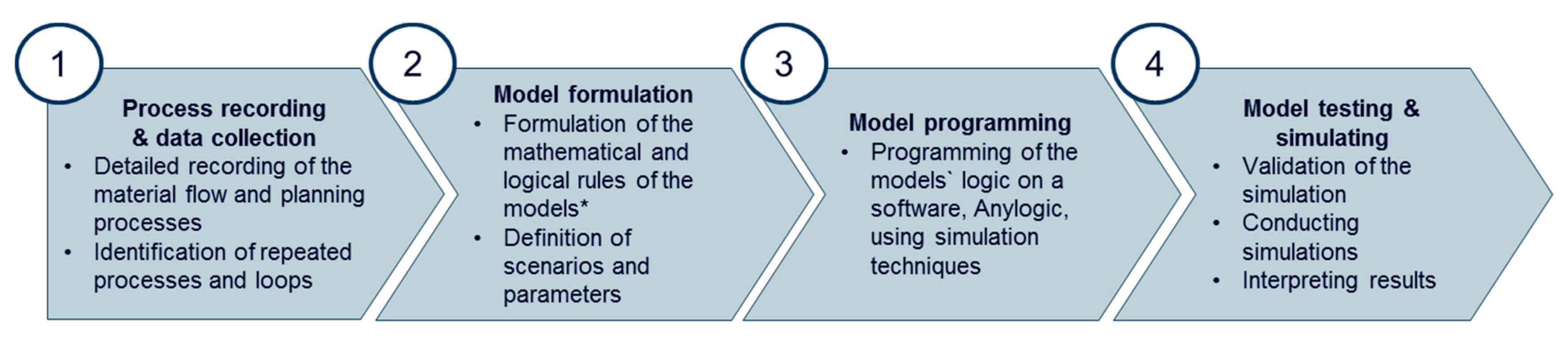
4. Applying the Model for Production Control to the Metallurgical Industry through Simulation

In order to make the decision and to increase the acceptance for future implementations in ETO manufacturers, an agent-based simulation was carried out in order to show the potential of this approach. The goal of this simulation is the comparison of today’s common production control logic, the push control logic, with potential pull control logic.

4.1. Process Recording and Data Collection

As explained the methodology the first step was to represent with a process mapping the material flow of the ETO metallurgical producer and associating the data to the specific processes and product families. The important representatives of the individual product families were depicted in a process mapping tool and then brought into the simulation model with their respective production routes. For each product family, the needs of five years were taken to design the base scenario. The agents that go through the simulation were the individual manufacturing positions or units with their parameters such as tons, volume, processing time per machine group, order release date, completion date, the transport times between machine groups, etc. In addition, these positions run through the various machine groups along its production. Each machine group includes a number of machines that manufactures the same products. The machine groups depend on their shift model, usually 15 or 21 shifts as explained before.

4.2. Model Formulation

Later, the logical differences between the models are to be described. Both models have the same assumptions as well as the same framework conditions:

• Time horizon: The tasks are assigned according to their temporal relevance at different planning levels. According to the St. Gallen management model, the strategic planning level has a planning horizon of several years [29] (p. 80). Based on it, five years were chosen for the simulation of the two models.
• Production mix: Seven different production families with 12 different production routes were considered.
• Finite capacity for all production steps. Production capacity as the sum of the capacities of the machines within a machine group.
• Processing times depend on the product family, on the variant of product family and on the weight of the production unit.
• Same transport times between buffers and machine independently of the product family.
• Infinite transport capacity between machines along the production process.
• Infinite stock capacity before, along, and at the end of the production process.
• Raw and operating materials are always available for the production process.
• Assumed that in 3 weeks a batch for a steel type can be produced.
• Quality problems or rework lead times are not considered.
• Personal planning not considered.
• Depending on the machine group, 15 or 21 shifts per week.
• Production units are the agents that flow along the production process.
• If the load of a bottleneck is too high, the units wait to get a release date. If there are a certain number of units waiting for it, the manufacturer loses the demand that influencing the bottleneck until the number of units falls below the limit.

Table 1. Differences between push and pull production control models for a metallurgical manufacturer.

No.	Difference	Push-Control	Pull-Control Applying TOC/DBR
1	Order release	Order release for improving capacity utilization in the first production steps	Regulated order release control based on the system load
2	Determination of delivery dates	Same order release for units of the same product family	Adjusted based on the system load
3	Sequence planning	First in First out (FIFO)	Global Priority Rule: Priority determined based on time consumption on the delivery date

describes the main differences between both models. The push control starts the production in the steel mill, as far as the orders are in the order intake, since it follows the principle that the machines must not remain still. This causes the production orders to start too early or too late, usually too early, and as a consequence, the WIP increases. In addition, the delivery date determination is not determined on the basis of the bottleneck resources per product family. This, together with a local optimization in the individual production steps, leads to situations with high stock, long lead times and poor on-time delivery.

On the other hand, in the pull control, order release into production is based on the load of the bottleneck resources. For each product family, there are certain typical bottleneck resources to analyze (e.g., indirect stock and direct stock before a machine group converted to processing hours). Indirect stock of a machine group is the stock that has to be processed by this machine group, which is already in production and that is not ready to initiate production in this machine group. By knowing the total amount of processing hours needed to process the direct stock and the indirect stock, the model can determine which one of the machine groups is a bottleneck resource. Therefore, delivery dates are determined by dynamic lead times, which are determined on the basis of the system load. The third difference is the introduction of a global priority rule, which forms the basis for sequencing before each production step. The priority of a position (%, as a percentage) is determined on the basis of the time consumption at the delivery date, the higher the priority the sooner the position has to be processed in that specific production step. This means that at every time period priorities are recalculated to create a list of next production units to be processed in each machine group to optimize the system globally by processing the critical units according to promised delivery date at first.

The two models have moving bottlenecks depending on the product mix that are in a particular moment in production process. The pull-control model can anticipate the bottlenecks by knowing the processing time needed in the current bottleneck resources. Based on this processing time a reliable delivery date is given.

The previously described characteristics are shown in Table 1.

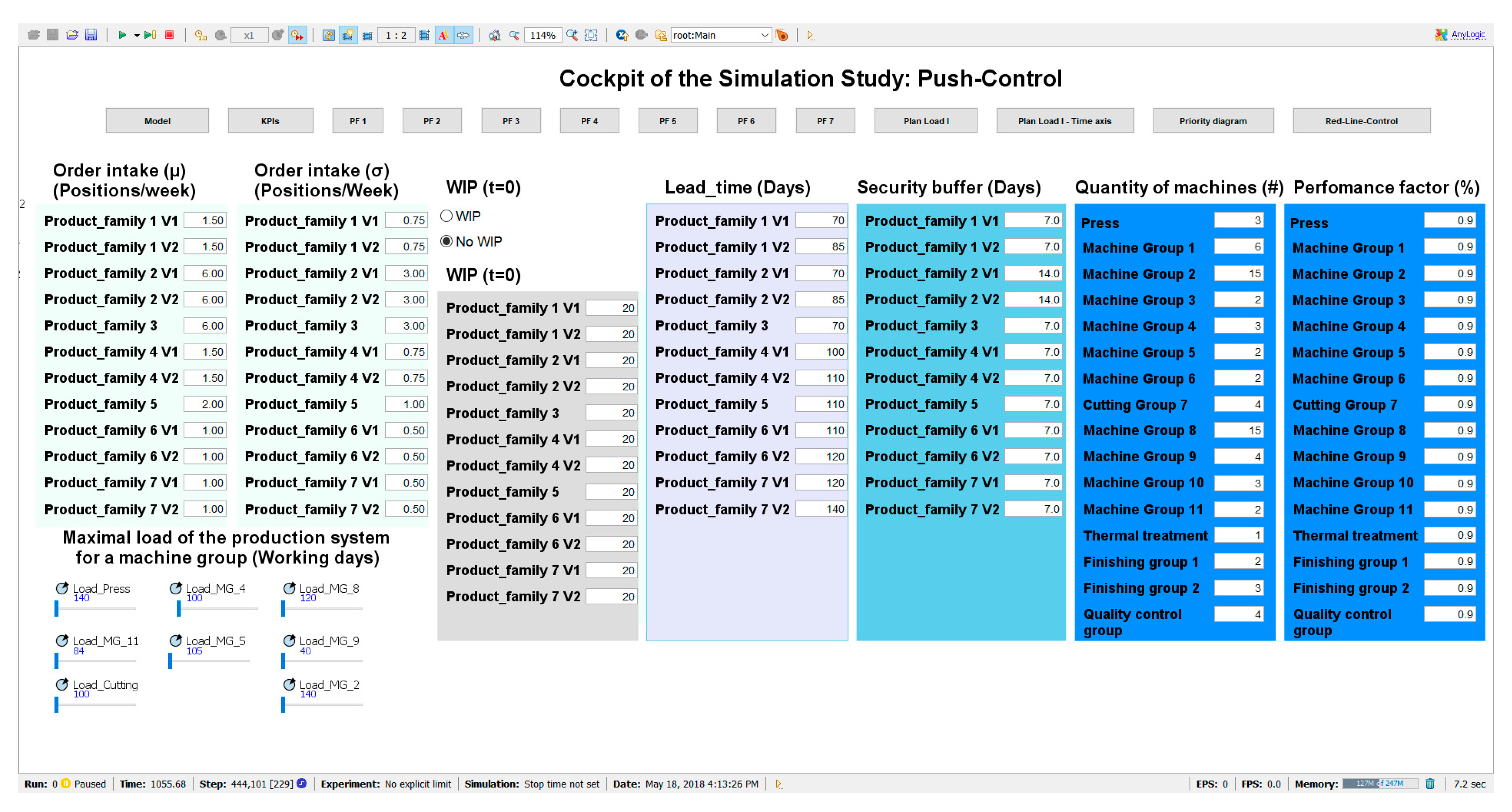
4.3. Model Programming

The simplified production flow simulated can be seen in Figure 4 below:

The models were created using delay times as lead times for production processes, transport, waiting times, etc. The AnyLogic software allows providing a processing time or delaying time depending on the agent entering in a machine group. When an agent or production unit enters a machine, the processing time that depends on the agent is activated. After this time the unit goes out of the machine and waits to be transported to the next processing step.

Moreover, the agents within the simulation are the production units with their parameters associated to them as listed below:

• Product family (number);
• Variant within the product family (number);
• Weight (tons);
• Processing lead time per production step (days);
• Days until security buffer (days);
• Transport lead times between all combinations of production steps (days).

Based on the flow of a production unit along its production process, the following parameters are calculated dynamically within the agents:

• Waiting time until order release is given (days);
• Promised production lead time (days);
• Production lead time (days);
• Transport lead time (days);
• Waiting times along the production process (days);
• Days before or after the promised production lead time (days).

Demand is created within the model with gamma distribution and is equal for both models. Its value is quantified according to the rate of incoming units or positions of a certain product family and variant and it is recalculated every 90 days, assuming that a certain pattern remains for 90 days.

The key performance indicators (KPIs) for the simulation model are:

• Demand: production units ordered (units). The value is written in an Excel file in periods of 90 days.
• Production units started: production units released (units). The value is written in an Excel file in periods of 90 days.
• OTD (on-time-delivery): percentage of units produced before the promised delivery date for logistics (%). The value is written in an Excel file in periods of 90 days.
• Production throughput: cumulated production (tons).
• WIP: quantity of units in production process (units).
• Stock before and after production process: quantity of units before and after the production process (units).

The KPIs per production family are: demand (units), OTD (%), production lead time since order release (days), lead times for technical processing, transport and waiting times (days), percentage of units that did not reach the security buffer (%), and the weight break-down of the units (tons and %).

The KPIs per machine group are: capacity utilization (%), planned load (weeks), priority of a unit before a machine group (%), and direct stock (weeks).

4.4. Model Testing and Simulating

The models can be initiated with WIP production units or without them depending on the adjustable parameters. Moreover, this and other adjustable parameters are shown in

Table 2. Adjustable parameters.

No.	Adjustable Parameter	Description	Unit
1	Demand	Expected value and deviation based on gamma distribution	Units per week
2	Maximal load per machine group	Production system load	Days
3	Production lead time	Time for production for the next orders	Days
4	Security buffer	Time for buffer for the next orders	Days
5	Quantity of machines	Number of machines per machine group	Machines
6	Shift model	Determines the planned production time	Shifts per week
7	Performance factor	Considers availability and performance losses	%
8	WIP at time = 0	Quantity of units in production process at day 0	Yes/No

:

Moreover, the values for the described parameters are to be introduced in the cockpit of the simulation model within the AnyLogic software, with the exception of the shift model that should be introduced in other screen within the model, as depicted in Figure 5:

In addition, Figure 6 shows the testing process performed within the simulation software:

5. Simulation Results and Implementation

The comparison was conducted with the following characteristics:

• Demand created within the model based on statistical distributions that are equal in both models.
• The following demand scenarios were performed are shown below in

  Table 3. Demand scenarios.

  No.	Scenario	Description	Name
  1	Scenario 1	Demand in an average level around 30 units per week	Base
  2	Scenario 2	High demand for all product families compared to base scenario	High
  3	Scenario 3	Low demand for all product families compared to base scenario	Low
  4	Scenarios 4–10	High demand for one product family and base for the others	High for product family X

  :
• Results are written in a “KPI (Key Performance Indicator)” Excel file and then compared between the models.

Results for all the scenarios were better for the pull-control with higher difference for scenario 2 and less difference for scenario 3. The results in

Table 4. Simulation results for push and pull-demand production control—base demand scenario.

No.	Key Performance Indicator	Push-Control	Pull-Control Applying TOC/DBR
1	OTD (%)	74	95
2	Production throughput (tons)	75	77
3	WIP (units)	339	285
4	Waiting time (%) from total production lead time	51	34
5	Capacity utilization (%)	58	61

are those for the base scenario, scenario 1, and show a clear competitive advantage for the pull control, as it had achieved better on-time delivery with less inventory and idle time at the same throughput. The biggest difference in the results happened when there was a large order intake. In this case, the pull control was able to smooth the demand with the determination of order release and completion dates, as it could act on the bottleneck early on, but the push-control could only react reactively when it was already too late:

6. Conclusions

This chapter was divided into theoretical, managerial, and empirical conclusions explaining also the limitations of the research performed as well as describing the potential research work derived:

Theoretical conclusions: the research paper pursued the following objectives, the improvement of the OTD (delivery schedules), the reduction of the stock in WIP and the reduction of the production lead times. In order to achieve these goals, a pull production control with a so-called “bottleneck control” was developed for an ETO manufacturer providing steps as guidelines to follow in order to apply it successfully in real manufacturers.

• A new concept using a TOC approach was developed.
• Steps for the implementation of the new concept developed were described.

Managerial conclusions:

• The current challenges of ETO manufacturers were described and those influencing the production system were integrated in the push control model.
• Internal efficiency was proved as key for metallurgical companies, in particular, for the steel industry.
• The importance of a controlled and synchronized communication between sales and production to assign realistic delivery dates that lead to higher customer satisfaction.

Empirical conclusions: to prove the utility of the new concept a simulation for a metallurgical example was created by including the necessary instruments and control systems developed as well as the validation by means of simulation. The model considered and simulated the variety of complex process such a batch production in the steelworks and unique production items in the other production steps as well as the interrelationships between them. That is why the planning and control system was robust, simple, and transparent to every employee and for the end-customer.

• Both concepts, pull and push-control, were implemented in AnyLogic software with agent-based modeling and simulated to compare the performance in different demand scenarios.
• The benefits of the change from a common push control approach to an approach using DBR are:

  ○

  Global optimization of the production system;

  ○

  Initiation of production with complete customer specifications;

  ○

  Shorter lead times;

  ○

  Higher delivery reliability;

  ○

  Lower inventories levels.

Limitations of the research work:

• Assumed that existing ETO producers used a production control based on a push approach.
• Complexity of an ETO manufacturer was partially built in the simulation model.
• Complexity of processes such as for steelmaking was not built in detail.
• Organization structure and interfaces were not considered in the simulation model.
• Quality problems were not considered.
• Concept was not proved in any company.

Future research: the potential research derived from this paper is:

• Transfer this research method to real production systems applying it in particular cases as an assistance tool for sales and production planning leaders and controllers by centralizing all data related to a topic in a short period of time enabling simulation of what-if-scenarios.
• Consider organization units and their communication within the simulation model.
• Improve the model from implementation feedbacks as well as apply it for production networks with several production plants.

To sum-up, the research work show the potential benefits of a capacity management based on a bottleneck control approach in which committed delivery dates can be met as well as improving internal production key performance indicators leading to an increase in competitiveness.

References

1. Hicks, C.; Mcgovern, T.O.M.; Earl, C.F. A Typology of UK Engineer-To-Order Companies. Int. J. Logist. 2001, 4, 43–56. [Google Scholar] [CrossRef]
2. Lacroix, Y.; Major Overcapacity in the Global Steel Industry. Major Overcapacity in the Global Steel Industry. Euler Hermes Economic Research. Economic Insight. 2013. Available online: http://www.eulerhermes.com/mediacenter/Lists/mediacenterdocuments/20131014_economic_insight_steel.pdf (accessed on 17 March 2014).
3. Price, A.H.; Weld, C.B.; El-Sabaawi, L.; Teslik, A.M. Unsustainable: Government Intervention and Overcapacity in the Global Steel Industry. 2016, pp. 1–25. Available online: https://www.wileyrein.com/media/publication/204_Unsustainable-Government-Intervention-and-Overcapacity-in-the-Global-Steel-Industry-April-2016.pdf (accessed on 29 December 2019).
4. Cao, W. An Empirical Study of the Impact of the “Cutting Overcapacity” Policy on the Performance of Steel Industry. DEStech Trans. Eng. Technol. Res. 2018. [Google Scholar] [CrossRef]
5. Steelmaking Capacity. ECD Steelmaking Capacity Database 2018. Available online: Retrieved from: https://stats.oecd.org/Index.aspx?DataSetCode=STI_STEEL_MAKINGCAPACITY (accessed on 29 December 2019).
6. World Steel Association. Steel Statistical Yearbook 2018. Available online: https://www.worldsteel.org/en/dam/jcr:e5a8eda5-4b46-4892-856b-00908b5ab492/SSY_2018.pdf (accessed on 29 December 2019).
7. Hicks, C.; McGovern, T.; Earl, C.F. Supply Chain Management: A Strategic Issue in Engineer to Order Manufacturing. Int. J. Prod. Econ. 2000, 65, 179–190. [Google Scholar] [CrossRef]
8. Lee, K.; Ki, J.H. Rise of Latecomers and Catch-Up Cycles in the World Steel Industry. Res. Policy 2017, 46, 365–375. [Google Scholar] [CrossRef]
9. Nozomu, K. Where Is the Excess Capacity in the World Iron and Steel Industry?—A Focus on East Asia and China; Research Institute of Economy, Trade and Industry: Tokyo, Japan, 2017; No. 17026. [Google Scholar]
10. Campuzano, F.; Mula, J. Supply Chain Simulation: A System Dynamics Approach for Improving Performance; Springer Science & Business Media: Berlin, Germany, 2011. [Google Scholar]
11. Borshchev, A. Simulation Modeling with Anylogic: Agent Based. Discret. Event Syst. Dyn. Methods 2013, 225–269. [Google Scholar]
12. Gosling, J.; Naim, M.M. Engineer-To-Order Supply Chain Management: A Literature Review and Research Agenda. Int. J. Prod. Econ. 2009, 122, 741–754. [Google Scholar] [CrossRef]
13. Westkämper, E. Einführung in die Organisation der Produktion; Springer: Berlin, Germany, 2006. [Google Scholar]
14. Hinckeldeyn, J.; Dekkers, R.; Altfeld, N.; Kreutzfeldt, J. Bottleneck-Based Synchronisation of Engineering and Manufacturing. In International Association for Management of Technology IAMOT 2010, Proceedings of the 19th International Conference on Management of Technology, Cairo, Egypt, 8–11 March 2010; Industry Committee of the International Association for Management of Technology: Cairo, Egypt, 2010. [Google Scholar]
15. Handfield, R.B. Effects of Concurrent Engineering on Make-To-Order Products. IEEE Trans. Eng. Manag. 1994, 41, 384–393. [Google Scholar] [CrossRef]
16. Lengnick-Hall, C.A. Innovation and Competitive Advantage: What We Know and What We Need to Learn. J. Manag. 1992, 18, 399–429. [Google Scholar] [CrossRef]
17. Kashan, A.J.; Mohannak, K.; Perano, M.; Casali, G.L. A Discovery of Multiple Levels of Open Innovation in Understanding the Economic Sustainability. A Case Study in the Manufacturing Industry. Sustainability 2018, 10, 4652. [Google Scholar] [CrossRef] [Green Version]
18. Rupo, D.; Perano, M.; Centorrino, G.; Vargas-Sanchez, A. A Framework Based on Sustainability, Open Innovation, and Value Cocreation Paradigms—A Case in an Italian Maritime Cluster. Sustainability 2018, 10, 729. [Google Scholar] [CrossRef] [Green Version]
19. Baláž, P.; Bayer, J. Impact of China on Competitiveness of EU Steel Industry (Slovakia). In Proceedings of the 4th International Conferenceon European Integration, Ostrava, Czech Republic, 17–18 May 2018; p. 118. [Google Scholar]
20. Hoitsch, H. Produktionswirtschaft: Grundlagen einer industriellen betriebswirtschaftslehre; Vahlen: Munich, Germany, 1985. [Google Scholar]
21. Schuh, G.; Brosze, T.; Brandenburg, U.; Cuber, S.; Schenk, M.; Quick, J.; Hering, N. Grundlagen Der Produktionsplanung Und-Steuerung. Prod. Und-Steuer. 2012, 1, 11–293. [Google Scholar]
22. Nyhuis, P. Produktionskennlinien—Grundlagen und Anwendungsmöglichkeiten; Springer: Berlin, Germany, 2008. [Google Scholar]
23. Wirtschaftslexikon, G. Stichwort: Produktionsprozessplanung; Verlag: Wiesbaden, Germany, 2013. [Google Scholar]
24. Chopra, S.; Meindl, P. Supply Chain Management. Strategy, Planning & Operation. Das Summa Summ. Des Manag. 2007, 265–275. [Google Scholar] [CrossRef]
25. Schuh, G.; Weber, H.; Kajüter, P. Logistikmanagement; Springer: Berlin, Germany, 2013. [Google Scholar]
26. Zäpfel, G. Grundzüge Des Produktions-Und Logistikmanagement Walter De Gruyter; De Gruyter Oldenbourg: Munich, Germany, 2001. [Google Scholar]
27. Hung, K.T.; Liou, E.D.; Wen, C.P.; Tsai, H.F.; Shi, C.S.; Chang, Y.C.; Lee, Y.J. Decision Support System for Inventory Management by TOC Demand-Pull Approach. In Proceedings of the 2010 IEEE/SEMI Advanced Semiconductor Manufacturing Conference (ASMC), San Francisco, CA, USA, 11–13 July 2010; pp. 23–26. [Google Scholar]
28. Jodlbauer, H.; Huber, A. Service-Level Performance of MRP, Kanban, CONWIP and DBR Due to Parameter Stability and Environmental Robustness. Int. J. Prod. Res. 2008, 46, 2179–2195. [Google Scholar] [CrossRef]
29. Bleicher, K. Das Konzept Integriertes Management: Visionen-Missionen-Programme; Campus Verlag: Frankfurt/Main, Germany, 2004. [Google Scholar]
Figure 1. Methodology used: steps.
Applsci 10 00274 g001
Figure 2. Simulation methodology used.
Applsci 10 00274 g002
Figure 3. Pull-production control logic.
Applsci 10 00274 g003
Figure 4. Simplified production flow of the simulation model: 6 main steps.
Applsci 10 00274 g004
Figure 5. Cockpit of the simulation study for the push-control model.
Applsci 10 00274 g005
Figure 6. Testing the model with the extreme-value test.
Applsci 10 00274 g006