Robust Speech Hashing for Digital Audio Forensics

Abstract

The verification of the integrity and authenticity of multimedia content is an essential task in the forensic field, in order to make digital evidence admissible. The main objective is to establish whether the multimedia content has been manipulated with significant changes to its content, such as the removal of noise (e.g., a gunshot) that could clarify the facts of a crime. In this project we propose a method to generate a summary value for audio recordings, known as hash. Our method is robust, which means that if the audio has been modified slightly (without changing its significant content) with perceptual manipulations such as MPEG-4 AAC, the hash value of the new audio is very similar to that of the original audio; on the contrary, if the audio is altered and its content changes, for example with a low pass filter, the new hash value moves away from the original value. The method starts with the application of MFCC (Mel-frequency cepstrum coefficients) and the reduction of dimensions through the analysis of main components (principal component analysis, PCA). The reduced data is encrypted using as inputs two values from a particular binarization system using Collatz conjecture as the basis. Finally, a robust 96-bit code is obtained, which varies little when perceptual modifications are made to the signal such as compression or amplitude modification. According to experimental tests, the BER (bit error rate) between the hash value of the original audio recording and the manipulated audio recording is low for perceptual manipulations, i.e., 0% for FLAC and re-quantization, 1% in average for volume (−6 dB gain), less than 5% in average for MPEG-4 and resampling (using the FIR anti-aliasing filter); but more than 25% for non-perceptual manipulations such as low pass filtering (3 kHz, fifth order), additive noise, cutting and copy-move.

1. Introduction

The proliferation of technologies and platforms for sharing information has made the increase in information in recent years exponential. Within this large amount of information, specific needs arise related to very diverse aspects such as authentication and integrity verification [1], content security [2], application of copyright [3], covert communication [4], or identification of multimedia contents [5], among others. Some of these applications fall within what is known as digital forensics.

Digital forensics is a discipline whose main objective is the application of computer tools in legal proceeding or an official investigation of some kind. It is used by experts to analyze, preserve and produce storage data for both volatile and non-volatile media, contributing to the veracity of digital evidence that is legally provided [6,7,8]. One of the fields of this discipline is audio forensics, where the aim is to acquire, analyze, or evaluate audio recordings which may be presented as admissible evidence in some official venue [9,10,11]. Some specific tasks normally performed in audio forensics include authentication and integrity verification and the identification of multimedia contents.

In the case of authentication and integrity verification applications, the aim is to ensure that the information (e.g., digital evidence) was not inadvertently or deliberately altered prior to examination, i.e., what is being demonstrated is that the content has not changed [9,12]. On the other hand, the identification of multimedia contents can be useful when there is only partial access to the information; this is the case of song identification systems (from a few seconds), or also of digital forensic systems, when the data have suffered fragmentation or partial destruction [13]. It is important to note here that the integrity check seeks to demonstrate that a content has not changed, while the multimedia content identification seeks to determine if the fragment is part of a content that has previously been identified as incriminating.

In any case, how these challenges are addressed depends on the characteristics and availability of information on the content to be evaluated. This is usually achieved through the calculation of a numerical value based on input data, i.e., the use of cryptographic hash functions [14]. However, due to the high sensitivity of these functions to minor changes in the input, this solution is not practical when exact copies of the content to be evaluated are not available [5]. This means that, if you only have partial access to content, or even if the content may have changed (e.g., in the file format), the solution is not appropriate. Similarly, alternatives such as encryption methods, cyclical redundancy check, or even meta-data use may fail when digital content is modified such as via file format conversion, meta-data removal, or analog/digital and digital/analog conversions [5,15].

In this type of situation, the methods that can be used must be robust enough to tolerate certain modifications, or even allow identification using only part of the contents [16]. These methods mainly include watermarking and robust hash functions. The first option is an invasive technique, consisting of the imperceptible insertion of a specific code over the content [17]. This option is valid when the content is susceptible to modification, but in some cases it may present drawbacks such as scalability or the need to previously mark all content to be evaluated [5]. In the case of robust hash functions, also known as perceptual hash functions or audio fingerprints, these are characterized as non-invasive. In this case, a static or at least almost insensitive behavior in the hash code with respect to permissible transformations in such content is desired [15].

In this context, the approach of robust hash functions for the identification of audio contents has aroused recent interest due to its multiple applications. For example, alternatives to perform audio identification by microphone capture have been presented [5], where one of the best known cases is that of Shazam, a company that has multiple patents in this regard [18,19]. Other cases include the identification of the audio environment to present related content (Google) [20], or in general, perceptual methods presented by companies such as Philips, Microsoft or Gracenote [5].

Different approaches to perceptual hash functions have also been presented in scientific literature. In general, perceptual hash methods may use one or more of the following blocks: (i) Divide the input signal into contiguous time windows with some overlap and apply some kind of analysis to them; (ii) separate the frequency components of the signal according to the human auditory system; (iii) apply some dimensional reduction technique. In the first case, different types of time-frequency transformations have been used, such as the FFT (fast Fourier transform ), DWT (discrete wavelet transform) [2,21], SWT (stationary wavelet transform) [22], modified discrete cosine transform [23], and Radon transform [24], among others.

In the second case, the use of techniques related to MFCC (Mel-frequency cepstrum coefficients) [25], SFM (spectral flatness measure), or SCF (spectral correlation function) have been proposed [5]. Finally, it is pertinent to use any size reduction technique that facilitates obtaining a short and constant code, for example using NMF (non-negative matrix factorization) [21,24] or PCA (principal component analysis). In [2], the authors use the approximation coefficients of a 3-level wavelet decomposition as the perceptual feature value, and a measurement matrix to reduce its dimension. According to the results, the approach shows improvements in terms of low pass filtering and MP3 compression. However, for lossy audio encoding the results are not consistent, as the error is lower for a low bit rate (average BER = 0.0042 for a 48 kbps bit rate), compared to a higher bit rate (BER = 0.2189 for a 128 kbps bit rate).

In any case, research related to perceptual hash functions is an active topic, mainly because tolerance to some types of modifications depends on the application. Therefore, there are still some challenges to be solved in this area. For example, in digital forensics it is required to identify content when the whole data is not available, or when the content has been manipulated through content-preserving operations (perceptual). Additionally, it is necessary to take into account the computational cost, both in the generation and in the process of searching for the hash value in a database.

Accordingly, this document proposes a new and robust hash function methodology for integrity verification in audio signals. In other words, what is expected is that the hash value be invariable or at least almost insensitive to moderate or permissible transformations in audio signals, such as format changes. This can facilitate chain of custody processes for digital evidence, even with unintended errors in the processing of information. The proposed method begins with the characterization of the speech signal by calculating the MFCC and reducing dimensions by PCA. Subsequently, the data given by PCA is encrypted, using as inputs, two values that come from a particular binarization system that uses the Collatz conjecture as a basis. Finally, a robust 96-bit code is obtained that can support input data modifications such as compression, amplitude modification, re-sampling and re-quantization.

The rest of the paper is organized as follows: Section 2 explains the concepts that will serve as a basis for the following sections. Section 3 presents the proposed method to summarize a speech signal. Section 4 shows the experimental validation, results and comparison of the proposed method. Finally, in Section 5 the conclusion is given.

2. Basic Concepts

2.1. Collatz Conjecture

The Collatz conjecture was enunciated by the German mathematician Lothar Collatz. It states that any positive integer (P) can be reduced to 1 by iteratively applying two operations (Equation (1)) that depend on the value of the entry number (even or odd). Its validation has been carried out partially [26], for which it is estimated that there may be an infinite number of exceptions [27,28]; however, its validity for small values ($P<2^{16}$) is easily verifiable.

$$\begin{array}{cc}{P}^{k+1}=\left\{\begin{array}{ccc}{P}^k/2& if& P^{k}iseven\\ 3\times P^k+1& if& P^{k}isodd\end{array}\right.,& P>1.\end{array}$$

(1)

2.2. MFCC

The MFCC (Mel-frequency cepstral coefficients) is a method to obtain a parametric representation of a signal, which has been widely used in speech recognition tasks. To obtain this representation, a 1st order FIR filter is used as a pre-emphasis filter to flatten the signal spectrum. Then, the STFT (short-time Fourier transform is applied to the signal, maintaining a time overlap between the frames. Its magnitude spectrum passes through a bank of filters formed by M triangular filters, where its linear frequency is assigned to Mel-frequency through Equation (2) [29].

$$Mel\left(f\right)=2595lo{g}_{10}\left(1+f/700\right).$$

(2)

In the Mel domain, the filters are equally spaced in a frequency band [29].

After signal filtering, the DCT (discrete cosine transform) is applied to the logarithm of the above data [30], in order to de-correlate them. Finally, a lifter is applied to obtain the MFCC coefficients. The MFCC has been applied to speech recognition, audio signal processing and other scenarios [31,32].

2.3. RSA

RSA (Rivest–Shamir–Adleman) is a well-known encryption algorithm that has been implemented in different security scenarios. This algorithm was created by Rivest, Adleman and Shamir and was patented in 1983 [33]; it is based on the generation of keys from two seed values (p and q), which are usually chosen as very high value prime numbers. This selection is based on the complexity involved in factoring very large numbers, which becomes more complex when the entry is a prime number. This method is an asymmetric algorithm, i.e., it uses different public and private keys. The encryption process of this algorithm can be summarized in the following six steps.

• Select two different prime numbers, named p and q.
• Calculate $n=p\times q$.
• Calculate the function $\varphi \left(n\right)=\left(p-1\right)\times \left(q-1\right)$.
• Randomly select an integer e, where $1<e<\varphi \left(n\right)$ and e is coprime with $\varphi \left(n\right)$.
• Calculate a private exponent d, where $1<d<\varphi \left(n\right)$.
• Apply module operation: $e\times dmod\varphi \left(n\right)=1$.
• Finally, public keys are e and n, and the private key is d.

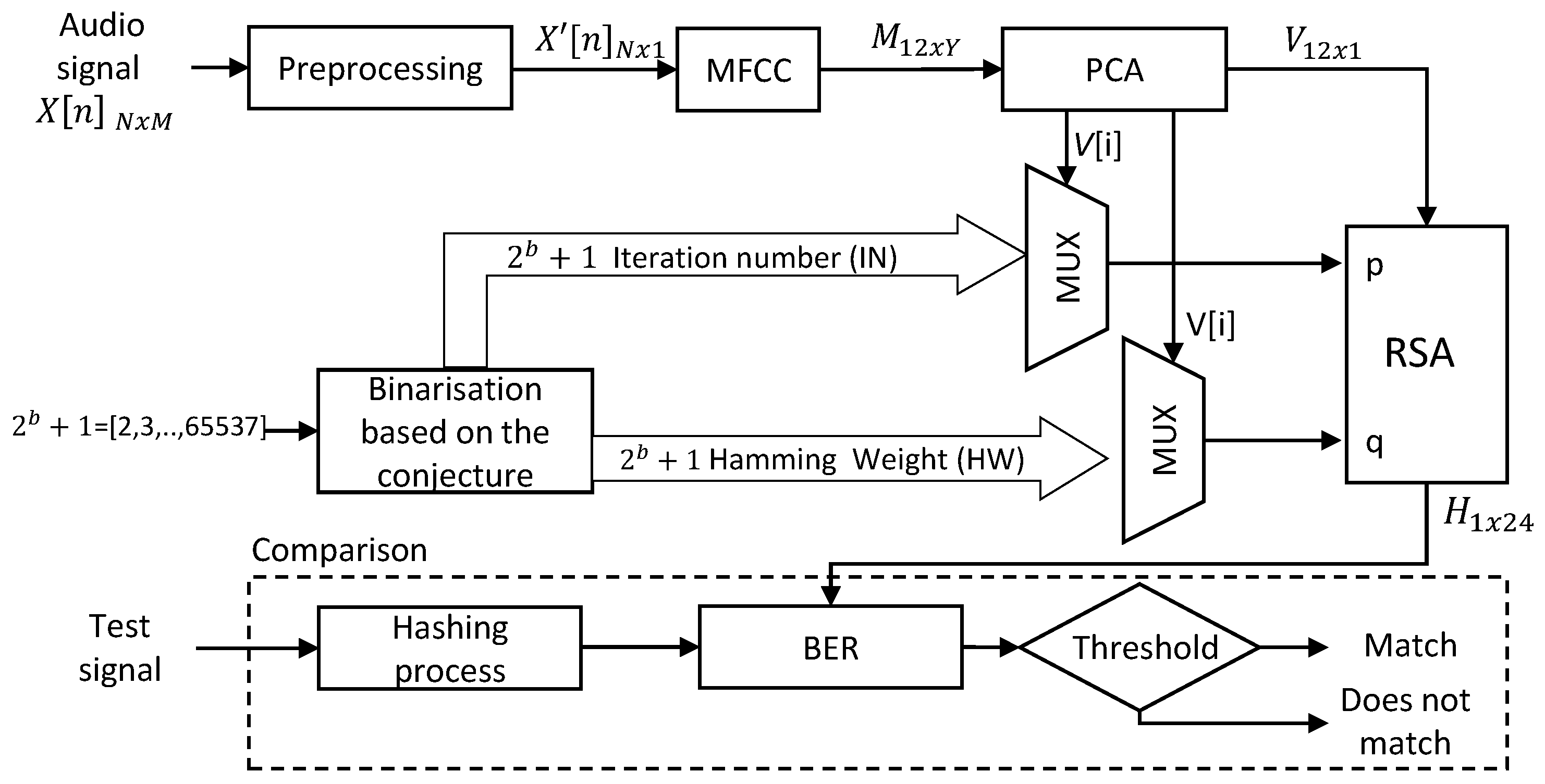
3. Proposed Method

The proposed method makes it possible to verify the integrity of a voice signal in forensic audio environments. The scheme summarizes a speech signal in a string with a fixed length. The proposed method can be explained according to the blocks shown in Figure 1.

3.1. Step 1. Pre-Processing

The input of the proposed scheme is a digital speech signal ($X[n,m],1\le n\le N,1\le m\le M$), where N is the number of voice samples of X, and M is the number of audio channels. The value of each sample is represented using a precision given by the number of bits per sample (b), and its value depends on the type of data (e.g., integer). The number of audio channels of this signal may be greater than one, so the first step is to convert $X\left[n\right]$ into a monophonic digital speech signal $X^{\prime }\left[n\right],1\le n\le N$.

3.2. Step 2. MFCC

Since the the proposed method is intended to be robust, it is proposed to use MFCC to obtain a representation of the signal as a function of the response of the human auditory system. The MFCC is a representation of the short-term power spectrum of the audio signal, where the short-term concept refers to the duration of the characteristics [34]. In the proposed method, the MFCC parameters are adjusted according to

Table 1. MFCC parameters.

Parameter	Value
Frame duration (ms)	500
Frame shift (ms)	250
Preemphasis coefficient	0.97
Number of filterbank channels	20
Number of cepstral coefficients	12
Cepstral sine lifter parameter	22
Lower frequency limit (Hz)	300
Upper frequency limit (Hz)	3900

.

The monophonic signal $X^{\prime }\left[n\right]$ is the input to the MFCC block, and its output is the matrix M ($12\times Y$). Here, the number of rows of M is the number of Cepstral coefficients configured in the MFCC block (which is set to 12), and the number of columns (Y) depends on the length of the input signal, according to the following Equation:

$$Y=⌊\frac{t}{FD-FS}⌋,$$

(3)

where t is the duration in seconds of the audio signal, $FD$ corresponds to the duration of the frame, and $FS$ corresponds to the frame shift in the MFCC block. In the proposed method, these parameters are $FD=500$ ms and $b=250$ ms, therefore Y is given by Equation (4).

$$Y=⌊\frac{t}{0.25}⌋-1.$$

(4)

3.3. Step 3. PCA

Once the MFFC matrix has been obtained, a reduction in dimensions is required. This process is done through PCA (principal component analysis), which decreases the amount of data through statistical analysis of input information. The process begins with the application of an orthogonal transformation to obtain a group of new uncorrelated variables, where the first component is characterized by having the greatest variance [35].

The application of PCA within the proposed method is carried out in order to reduce the number of observations in the M matrix, thus obtaining at the output a single vector V of 12 elements (corresponding to the number of coefficients of the MFCC block). In other words, PCA is being applied in time frames. Although the dependence of the samples of the original audio signal is strong, the application of PCA is proposed based on the following two reasons:

• In time series data, the closer the vectors are (in time), the greater the dependency, and vice versa [36]. Since the columns in matrix M correspond to 250 ms window frames (FD–FS), the time separation of these frames is greater than the corresponding separation of the samples in the original signal ($1/samplingfrequency=1/8000=125\mathsf{\mu }s$).
• The main purpose of the proposed hash function is descriptive, not inferential, i.e., to summarize the data. Therefore, non-independence does not seriously affect the application of the PCA [36].

Finally, each element of vector V is represented in integer format with b-bit precision. Its value will be masked using the values supplied by the binarization block.

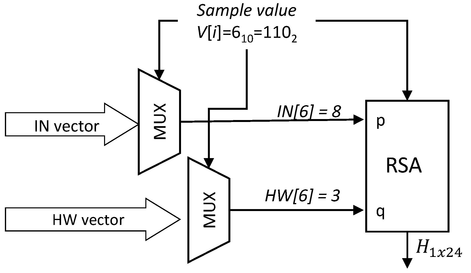
3.4. Step 4. Binarization Based on the Collatz Conjecture

The purpose of this block is to generate the data that will serve as input to the encryption algorithm based on RSA. For the generation of this data, it is proposed to use the Collatz conjecture for the binarization of integer values. From the conjecture, it is possible to obtain an alternative binary representation of positive integers. In each iteration of the reduction process, a bit is added depending on which of the two expressions is used, i.e., when the operation applied is $L/2$, a bit “0” is added, otherwise a bit “1” is added. Two additional values are obtained from the binary vector. The first is the number of iterations ($IN$) that the algorithm uses to reduces the integer to 1. The second is the Hamming weight ($HW$) of the binary vector, i.e., the number of ones in the vector.

In the example shown in

Table 2. Example of Collatz conjecture-based binarization.

$\mathit{X}=6$	Operation	Binary Vector
6	$6/2=3$	0
3	$3\times 3+1=10$	1
10	$10/2=5$	0
5	$5\times 3+1=16$	1
16	$16/2=8$	0
8	$8/2=4$	0
4	$4/2=2$	0
2	$2/2=1$	0
1		1 (MSB)

, the Collatz conjecture has been applied to reduce the number six. The results are the binary vector “100001010”, $IN=8$, and $HW=3$.

Given that the elements of the vector V are represented in integer format with a precision of b bits, in the binarization block, the objective is to obtain a set of $IN$ and $HW$ values that allow each of the possible values that V can take to be represented. In this case, this block provides $2^b$$IN$ and $HW$ values. Each pair of values is obtained through the algorithm shown in Algorithm 1. It is important to bear in mind that the vectors containing the $IN$ and $HW$ values are only generated once.

Algorithm 1 Collatz-Based Binarization.

1: Input:$X,L\leftarrow 2,Cont\leftarrow 0.$ 2: Output:$Vector\_Bin,IN,HW.$ 3: $Vector\_Bin\leftarrow \left[\right];$ 4: whileX ≠ 1 do 5:  if X is even then 6:   $X\leftarrow X/2$ 7:   $Vector\_Bin\leftarrow [0Vector\_Bin]$ 8:  else 9:   $X\leftarrow 3\ast X+1$ 10:   $Vector\_Bin\leftarrow [1Vector\_Bin]$ 11:  end if 12: end while 13: $IN\leftarrow lengthofVector\_Bin$ 14: fori ← 1 to IN do 15:  $HW\leftarrow HW+Vector\_Bin\left(i\right)$ 16: end for

The next step is to replace each element in the vector V using the $IN$ and $HW$ values. To obtain the values corresponding to each V element, two multiplexers are used. In the first multiplexer, the b bits of the V element are used as select lines and each of the $2^b$$IN$ values are the input lines; in the second multiplexer, the select lines are the same, while the input lines are the $2^b$$HW$ values. This means that a value of j in V, is replaced by the $j^{th}$ position in $IN$ and by the $j^{th}$ position in $HW$. Both the $IN$ and $HW$ values of each element in V will be used as input values for the encryption block.

Continuing with the previous example, the sample value is replaced by two values: The number of iterations and the Hamming weight (see Figure 2). In this case, the value of the select lines of the upper multiplexer is 6, so the output value corresponds to the sixth element of the vector IN, i.e., the number of iterations for the number 6 in the Collatz-based binarization. Similarly, the value of the select lines of the lower multiplexer is 6, so the value of its output is the sixth element of the HW vector, i.e., the hamming weight of the number 6 in the Collatz-based binarization.

3.5. Step 5. RSA Encryption

The last block in the proposed method is RSA. This block has three entries, the vector V, and the values p and q. For the proposed algorithm, the inputs p and q correspond to $IN$ and $HW$, respectively.

It should be noted here that, although these values are not very high, computational complexity remains, as each sample is independently coded (i.e., with different p and q). In addition, both $IN$ and $HW$ can present similar values for each value of V. Additionally, the proposed methodology could be used with another encryption method that uses seed values for key generation. In any case, what best ensures that the method is not reversible is not the encryption itself, but the extraction of characteristics by MFCC and data reduction by PCA.

Finally, from the keys generated with each p and q, the encryption of each value of V is carried out, having as output the data encrypted by RSA, called $H\left[i\right]$. This output is a fixed-length string containing 96 bits, i.e., a 24-digit hexadecimal string.

3.6. Step 6. Comparison

After obtaining the hash code, it is possible to compare it with the hash code of a second test signal. The hash value of this second signal is obtained using the same method as explained above, and their comparison is made using the BER. The threshold analysis that determines whether the signals match is presented in Section 4.4.

4. Experimental Results And Analysis

4.1. Experimental Dataset

The speech recordings used in the validation of the proposed method come from a proprietary dataset of 500 audio recordings from Spanish and English speakers. Each file is monophonic, with a length between 24 and 59 s, a sampling frequency of 8 kHz and 16 bits per sample.

4.2. Performance Analysis

Performance analysis of the hash function is presented in terms of BER (bit error rate) and ER (entropy rate). BER and ER are defined below.

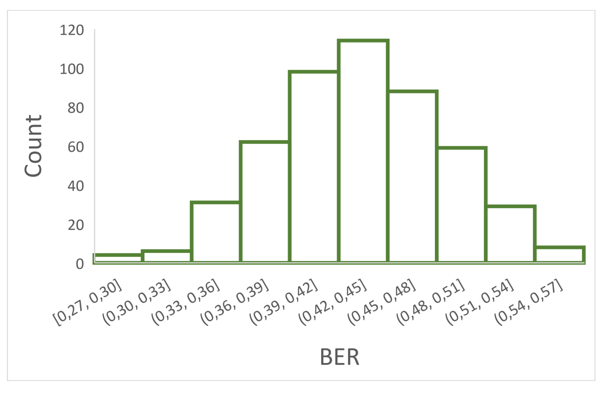
• Bit Error Rate (BER): One of the widely used parameters for comparing a pair of hash codes is the BER. It is equal to the number of bits that differ between two hash codes, divided by the length of the hash sequence. The maximum value of BER is 1 and the minimum is 0. In the first case the two hash codes are completely different, while in the second case the codes are the same.
  The formula for obtaining the BER is:

  $$BER=\sum _{i=1}^N\frac{h_1\left(i\right)\oplus h_2\left(i\right)}{L},$$

  (5)

  where $h_1$ and $h_2$ are the hash codes of two different recordings, L is the length of the hash value, and ⊕ is the XOR operator.
  In this study, with 500 different recordings (a), the number of BER values obtained with all available pairs is calculated using the binomial coefficient:

  $$\left(\begin{array}{c}a\\ b\end{array}\right)=\frac{a!}{b!\left(a-b\right)!},$$

  (6)

  for $a=500$, $b=2$. Then, our result is $500!/(2!498!)=500\times 499/2=124,750$. Having many BER values, they should follow a Gaussian distribution with $\mu =0.5$ and $\sigma =\sqrt{\mu \left(1-\mu \right)/L}$ [37]. Since $a=500$, $L=96$, the expected standard deviation value will be $\sigma =\sqrt{0.5\left(0.5\right)/96}=51\times {10}^{-3}$. As a result, Figure 3 shows the histogram of 499 BER values obtained by the comparison between a sample recording and the rest of the remaining 499 recordings.
  Table 3. Expected values (${}_t$) and experimental values (${}_e$) obtained from the entire 124,750 BER values.

  Type	Theoretical Values		Experimental Values
  Parameter	${\mu }_t$	${\sigma }_t$	${\mu }_e$	${\sigma }_e$
  Value	0.5	0.05103	0.4175	0.05439

  shows the expected values and experimental values obtained from the 124,750 BER values. As can be seen in this Table, with the proposed hash function, the data distribution approximates the Gaussian distribution. This function facilitates resistance to collisions since both the mean and the dispersion of bits that differ between two hash codes of different recordings are close to the theoretical value.
• ER (entropy rate). The ER value allows you to compare the performance of hash functions and, unlike other evaluation parameters, does not depend on the length of the hash code. The higher the ER value, the better the performance. The ER is obtained by taking into account the probability of transition between two hash sequences, p, using the following equation:

  $$ER=-p{log}_2\left(p\right)-\left(1-p\right){log}_2\left(1-p\right),$$

  (7)

  where $p=0.5\left(\sqrt{{\sigma }_e^2-{\sigma }_t^2/{\sigma }_e^2+{\sigma }_t^2}+1\right)$. For our case, $p=0.626$, and therefore $ER=0.953$. These values are discussed in Section 4.5.

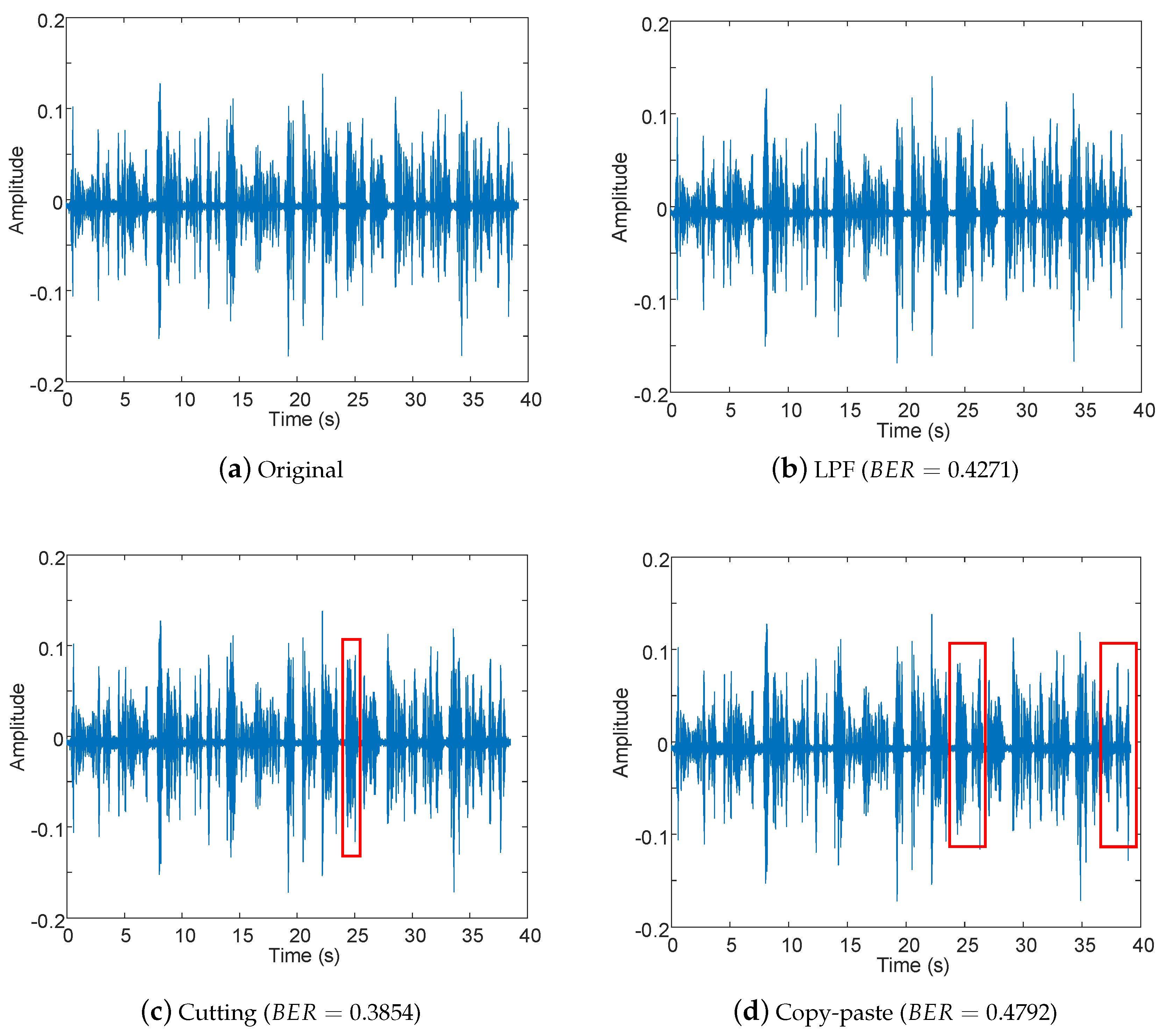
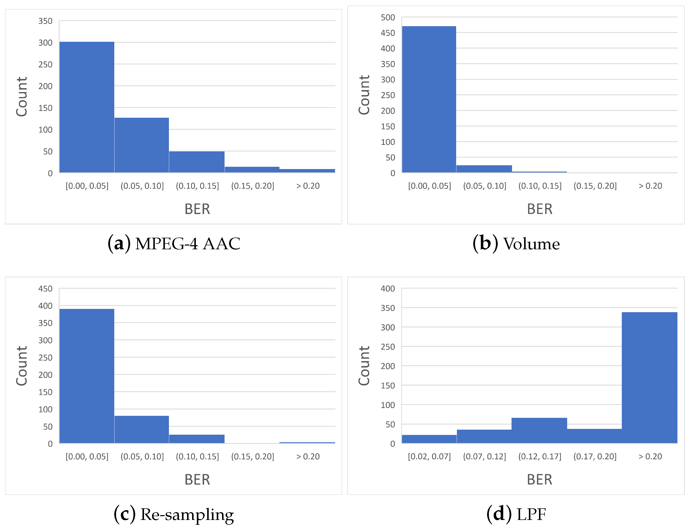
4.3. Analysis with Perceptual and Non-Perceptual Manipulations

Once the hash codes of different recordings have been analyzed theoretically and experimentally, the next step is to examine the hash codes after applying perceptual and non-perceptual manipulations. The first ones preserve the content, i.e., that do not change the perceived content. Generally speaking, two audio clips can be considered significantly similar if they sound the same [38]. For forensics purposes, it is desirable that perceptually similar recordings have very similar hashes (i.e., a BER close to 0), while for non-perceptual manipulated recordings they have dissimilar hashes (i.e., a BER close to 50%).

In order to illustrate BER values for perceptual and non-perceptual manipulations, we apply the following tests: FLAC, MPEG4 AAC, volume, re-sampling and re-quantization (perceptual), and LPF, additive noise, cutting and copy-move (non-perceptual).

Table 4. Manipulations used to test perceptual and non-perceptual hashing.

Perceptual Manipulation	Description	Parameters
Format conversion: FLAC	Conversion to FLAC and returned to wav	Sample rate: 8 kHz Bits per sample: 24
Format conversion: MPEG-4 AAC	Conversion to MPEG-4 AAC and returned to wav	Sample rate: 44.1 kHz BitRate: 192 kbps
Decrease Volume	The amplitude of the recording is attenuated by a scale of 2	Gain: −6 dB
Re-sampling	Sampling frequency is set to 16 kHz and returned to 8 kHz	8 kHz → 16 kHz → 8 kHz (using anti-aliasing FIR filter)
Re-quantization	Each sample is quantized to 32 bits/sample, and returned to 16 bits/sample	16 bits → 32 bits → 16 bits
Low-pass filtering	Butterworth low pass filter (LPF)	3 kHz, fifth order
Noise	Gaussian Additive noise	$\mu =0\sigma =0.01$
Cutting	Delete samples from the original signal	5000 samples are deleted
Copy-move	Copy and move samples in the original signal	10,000 samples are exchanged

describes the parameters used in each case. To illustrate an example, the signal shown in Figure 4a was used. In the case of perceptual manipulations, both the RMS (root mean squared) value of original minus modified signal, and the BER between the hash of the modified signal and the hash of the original signal were calculated (see

Table 5. Example of perceptual manipulations for original signal shown in Figure 4a: RMS (root mean squared) values of original signal and original minus modified signal.

Signal	RMS Value
Original	$179\times {10}^{-4}$
Original − Flac	0
Original − MPEG-4 AAC	$1.502\times {10}^{-4}$
Original − Volume	$89\times {10}^{-4}$
Original − Re-sampling	$0.658\times {10}^{-4}$
Original − Re-quantization	0

and

Table 6. Example of perceptual manipulations for original signal shown in Figure 4a: BER values of original signal versus modified signal.

Signal	BER
Original	0%
Flac	0%
MPEG-4 AAC	10.42%
Volume	4.17%
Re-sampling	1.04%
Re-quantization	0%

, respectively). According to these results, although RMS values can be higher than zero for perceptual manipulations, their BER values are lower than 11%. On the other hand, Figure 4 shows examples of non-perceptual manipulations, with BER values higher than 38%. This means that the hash values of signals with perceptual manipulations are similar to the hash value of the original signal, whereas for signals with non-perceptual manipulations, the hash values differ greatly from the original hash value.

For the second part of the test, for each of the manipulations listed in Table 4, 500 manipulated signals, their hash value and their BER were obtained. The average BER for each manipulation is presented in

Table 7. Results of perceptual and non-perceptual tests for 500 signals.

Manipulation	Average of BER Values
FLAC	0.00%
MPEG-4 AAC	4.79%
Volume	0.99%
Re-sampling	2.75%
Re-quantization	0.00%
LPF	26.44%
Noise	41.62%
Cutting	33.45%
Copy-move	33.05%

. According to these results, for perceptual manipulations the BER value (in average) is lower than 5%, while for non-perceptual manipulations it is higher (in average) than 25%.

In addition to the BER average, it is important to know the complete behavior of the data for each type of manipulation. Figure 5 shows the histograms of BER values for the manipulations where the hash differs.

As can be seen in Figure 5, the first three histograms are highly concentrated around the first bin, with more than 60% of the data. Only a few BER values are in the last bin (>0.20). This behavior is highly desirable for the perceptual hash, as it allows a threshold to be set for separating recordings with different content from perceptually similar files. On the other hand, in non-perceptual manipulation (Figure 5d), most BER values are in the last bin (>0.20), which means that the hash value has changed a lot, and it will not be easy to discern whether the contents match.

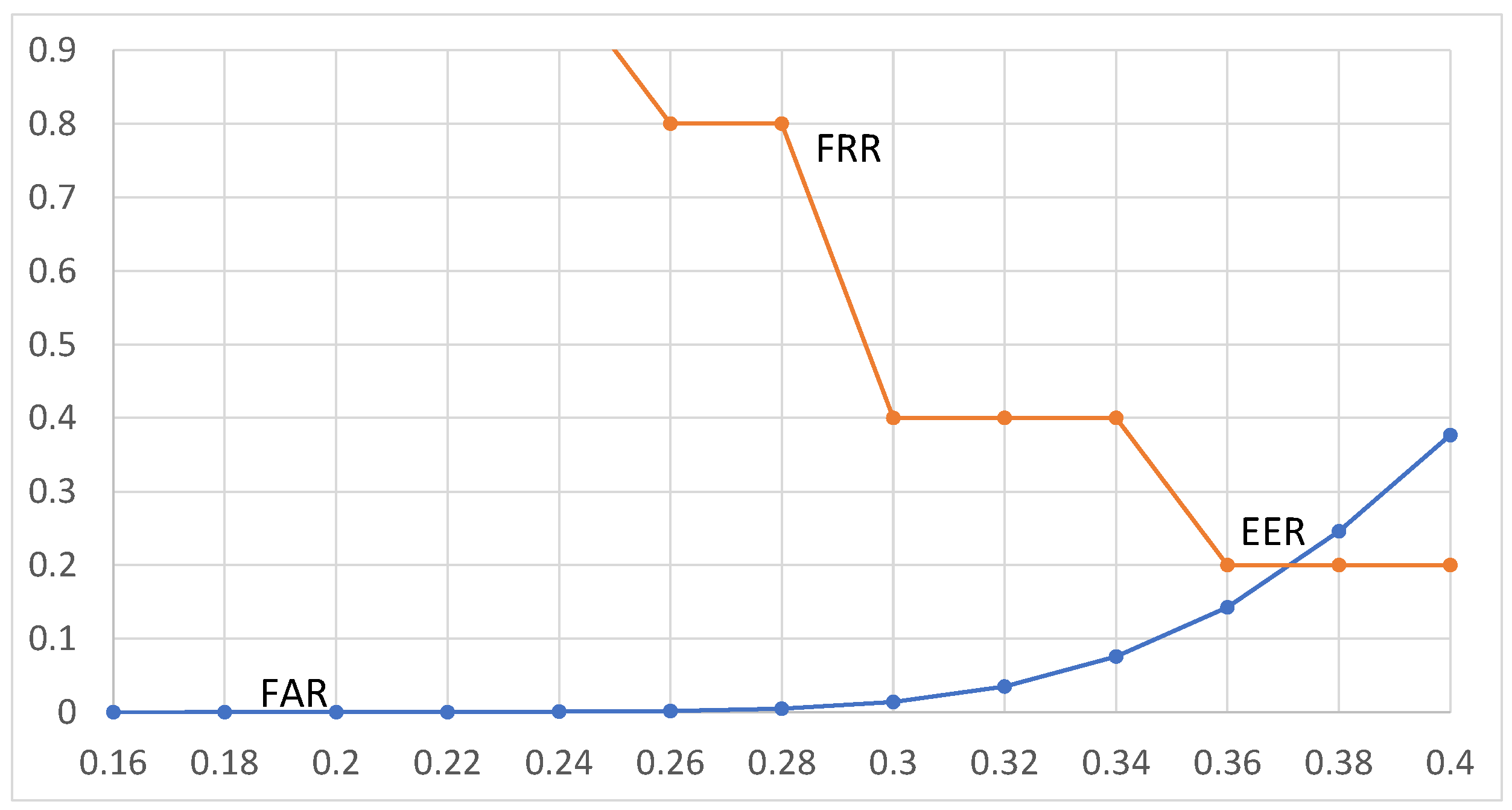
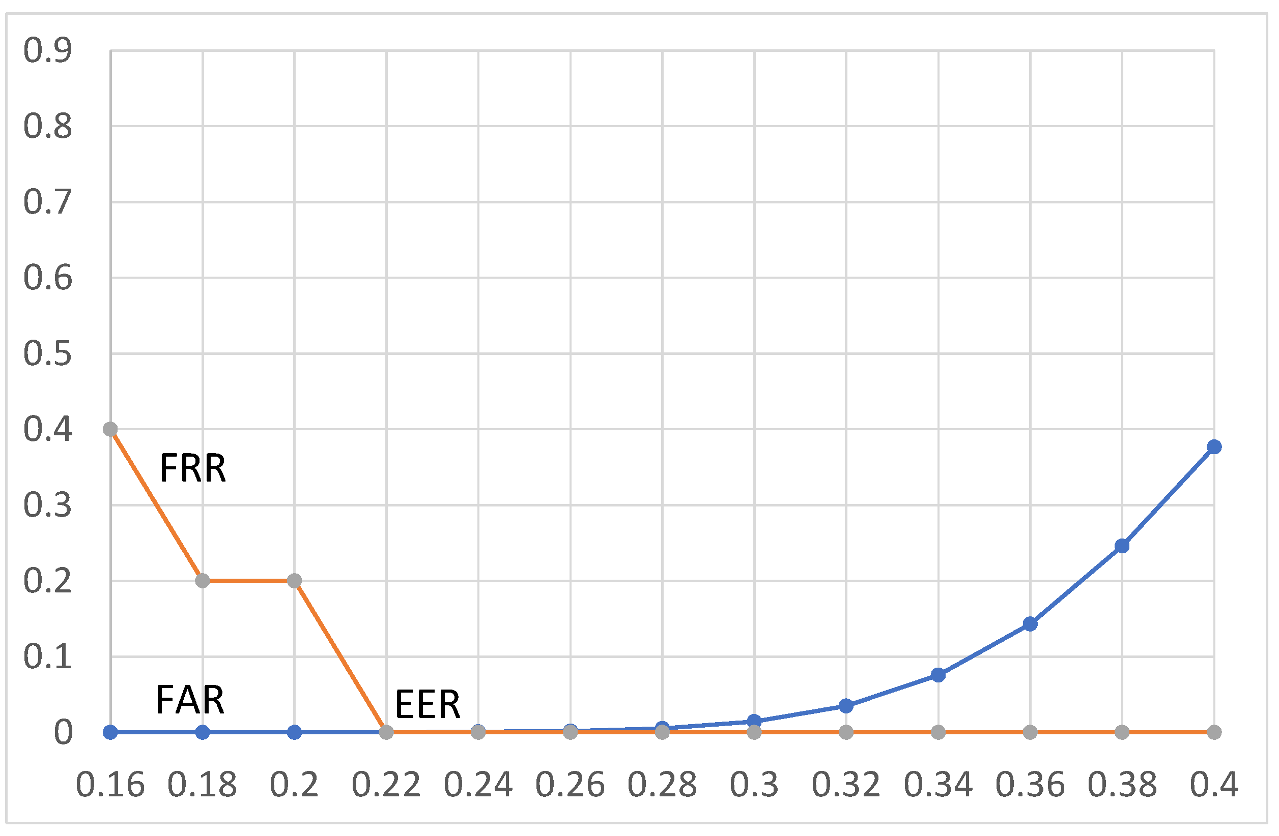
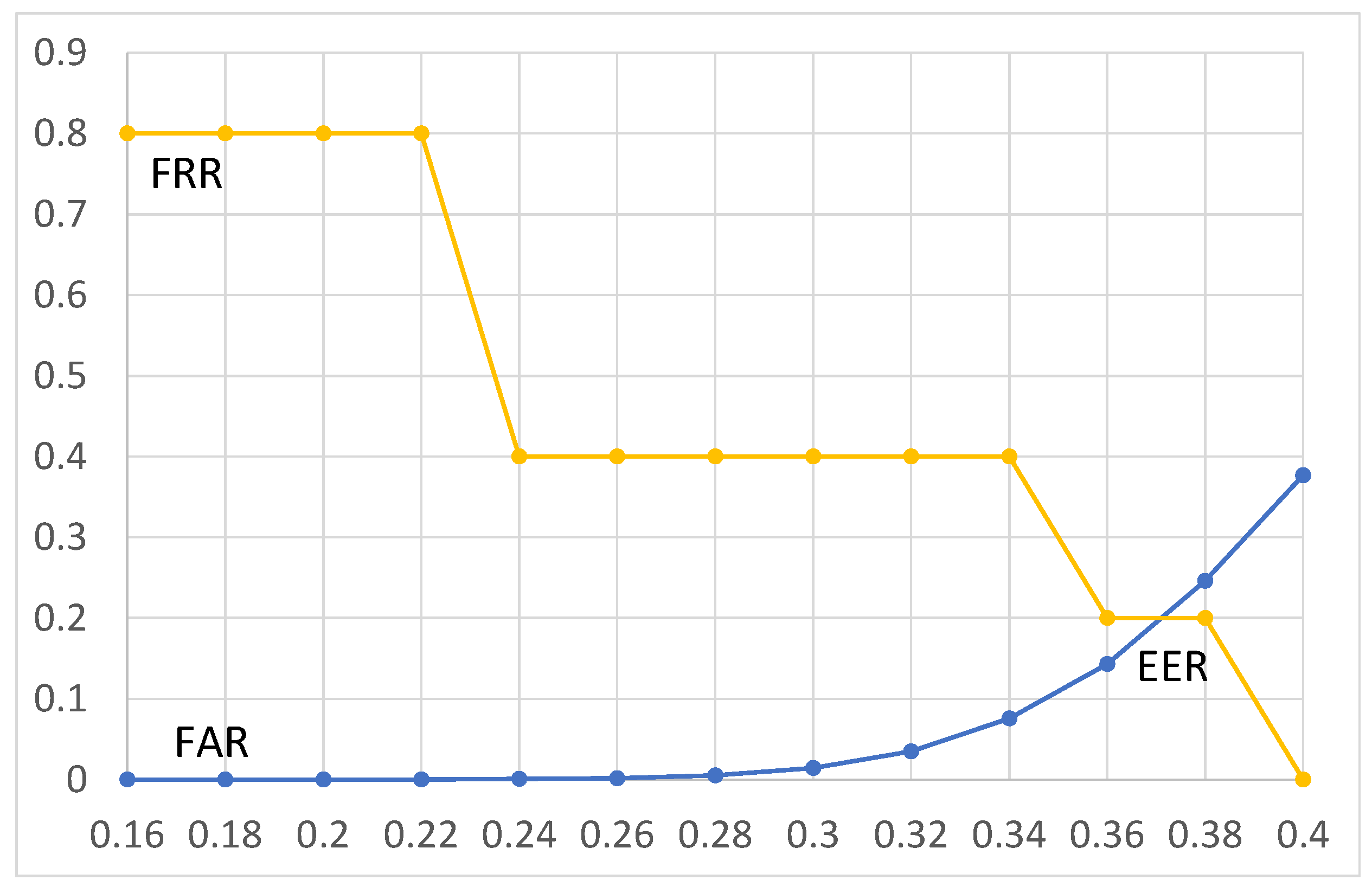
4.4. EER (Equal Error Rate) and the Threshold (th)

The last step in adjusting our model for perceptual purposes is the selection of the threshold. The aim is to differentiate recordings with different content and to detect files with perceptual manipulation. This is achieved by balancing FAR (false acceptance rate) and FRR (false rejection rate). FAR is the ratio of the number of false acceptances (i.e., when two recordings of different content are classified as perceptual modification) to the number of attempts, while FRR is the ratio of the number of false rejections (i.e., when two recordings with the same perceptual content are classified as different content) to the number of attempts. For forensic purposes, FAR implies that a new recording can be used as (false) evidence and FRR implies that evidence that has been perceptually manipulated can be discarded as valid evidence. Neither case is desirable, so it is necessary to find the best point where both parameters have the same value, i.e., the EER.

Figure 6, Figure 7 and Figure 8 show the FRR and FAR values for different threshold values for each type of perceptual manipulation.

For MPEG-4 AAC manipulation, according to Figure 6, the EER value is obtained when the threshold is 0.37, where the values of FAR and FRR are equal to 0.2%. It should be noted that for threshold values lower than EER, the value of FAR is extremely low, and for threshold values higher than EER, the value of FRR decreases. EER is the trade-off between both performances. The above results mean that discrimination between perceptual manipulation or different content is correct in the 99.8% of cases (i.e., 100 − EER). It is also worth noting that with 124,750 BER values, the resolution is $1/124,750=8\times {10}^{-6}$; for 500 BER values, the resolution is $2\times {10}^{-3}$. This means that with this dataset, the lowest possible values of FAR and FRR are $8\times {10}^{-4}$% and 0.2%, respectively.

In terms of volume adjustment, for th = 0.22, the FRR equals 0% and the FAR equals $208\times {10}^{-6}$%. Since the resolutions of FRR and FAR are not equal, the threshold of 0.22 is assigned as point EER, with a value of $208\times {10}^{-6}$%. The use of this threshold results in discrimination between perceptual manipulation and different content being correct in 99.9979% of cases.

For re-sampling manipulation, the EER value is 0.2% for a th = 0.37. The discrimination accuracy is equal to the MPEG-4 AAC compression case.

It is important to note that both FLAC manipulation and re-quantization work without false classifications. This means that, despite the threshold value, in all cases the data are correctly classified.

4.5. Comparison with Related Works

In this section, we compare the proposed method with others of the state-of-the art. The following parameters are selected: Volume adjustment (attenuation), re-quantization (up), downsampling and ER.

Table 8. Comparison with state-of-the art approaches.

Perceptual Modification	Ours	[37]	[23]	[2]	[39]	[40]
Volume adjustment	$98\times {10}^{-4}$	$78\times {10}^{-3}$	$98\times {10}^{-3}$	$46\times {10}^{-6}$	0	$78\times {10}^{-5}$
Down-sampling	$27\times {10}^{-3}$	0	$27\times {10}^{-3}$	$11\times {10}^{-4}$	$52\times {10}^{-2}$	$37\times {10}^{-4}$
Re-quantization	0	NP	$11\times {10}^{-5}$	0	$3\times {10}^{-2}$	NP

and

Table 9. Comparison in terms of entropy rate.

Parameter/Method	${\mathit{\sigma }}_{\mathit{t}}$	${\mathit{\sigma }}_{\mathit{e}}$	P	ER
Ours	0.051	0.054	0.626	0.953
[24]	0.0264	0.0366	0.781	0.758
[40]	0.0316	0.0341	0.637	0.944

show the results.

According to the results of Table 8, the proposed method is the most effective in handling re-quantization; it has an intermediate position for volume adjustment, as well as for down-sampling. The previous works do not provide information regarding conversion to FLAC and MPEG-4 AAC. In our case, FLAC compression does not change the hash value, whereas for MPEG-4 AAC, the mean BER value is $47\times {10}^{-3}$. Here it is important to take into account both the mean and the standard deviation of the BER values. A high $\sigma$ value may imply the appearance of FAR or FRR.

For the above reasons, the values of p and ER are also taken into account. The closer ${\sigma }_e$ is to ${\sigma }_t$, the better the performance of the hash function, then $p_e$ is more similar to $p_t$, i.e., 0.5, and as a consequence, the ER value is closer to 1 (ideal). In other words, if the dispersion of BER values is significantly greater than the theoretical value, the system does not work with an adequate transition probability between two hash values nor does it distinguish between ability and compression rate. Table 9 shows the results for some selected state-of-the-art methods.

According to the results of Table 9, the proposed method has a high entropy rate value, and therefore, the proposed hash function follows the suggested characteristics for perceptual applications.

5. Conclusions

The most important challenge of current research in verifying the integrity of digital audio evidence was to provide a control function that would tolerate manipulations of signals with preserved content, but would also identify those that significantly modified the content. For example, the hash value of an altered recording with volume adjustment should be very similar to that of the original recording, but the signal filtered with an LPF should provide a hash value distant from the original. Thus, we proposed a method that summarizes the audio signal, but at the same time identifies its most significant patterns, through the MFCC, PCA and RSA blocks. Since hash values are sensitive to changes in the audio signal, it was necessary to define the BER threshold value between the hash of the original audio and the hash of the manipulated audio in order to provide a binary output in relation to the integrity of the content. The methodology to determine the threshold values was through the cut-off point between FRR and FAR, in such a way as to optimize the number of manipulated audio files that were labelled as authentic versus the number of original audio recordings that were labelled as non-authentic. According to the results, the accuracy in verifying the integrity of the audio recording is greater than 99.8% for the following manipulations: FLAC (sampling frequency: 8 kHz, and 24 bits per sample), MPEG-4 (sampling frequency: 44.1 kHz, and bit rate: 192 kbps), volume adjustment (Gain: −6 dB), resampling (8 kHz → 16 kHz → 8 kHz), re-quantization (16 bits → 32 bits → 16 bits), LPF (3 kHz, fifth order), additive noise, cutting and copy-move.

For future work, we propose the testing of hash values with other types of manipulations such as acoustic impulse responses, and determining of the appropriate BER threshold value.

References

1. Renza, D.; Ballesteros, D.; Lemus, C. Authenticity verification of audio signals based on fragile watermarking for audio forensics. Expert Syst. Appl. 2018, 91, 211–222. [Google Scholar] [CrossRef]
2. Zhang, Q.; Qiao, S.; Huang, Y.; Zhang, T. A high-performance speech perceptual hashing authentication algorithm based on discrete wavelet transform and measurement matrix. Multimed. Tools Appl. 2018, 77, 21653–21669. [Google Scholar] [CrossRef]
3. Fallahpour, M.; Megias, D. Audio Watermarking Based on Fibonacci Numbers. IEEE/ACM Trans. Audio Speech Lang. Process. 2015, 23, 1273–1282. [Google Scholar] [CrossRef]
4. Renza, D.; Ballesteros, D.M.; Ortiz, H.D. Text Hiding in Images Based on QIM and OVSF. IEEE Lat. Am. Trans. 2016, 14, 1206–1212. [Google Scholar] [CrossRef]
5. Gonzalez, F.P.; Alfaro, P.C.; Freire, L.P.; Vieites, D.P. Method and System for Robust Audio Hashing. U.S. Patent 9,286,909, 15 March 2016. [Google Scholar]
6. Meyers, M.; Rogers, M. Computer forensics: The need for standardization and certification. Int. J. Digit. Evid. 2004, 3, 1–11. [Google Scholar]
7. Delp, E.; Memon, N.; Wu, M. Digital forensics [From the Guest Editors]. IEEE Signal Process. Mag. 2009, 26, 14–15. [Google Scholar] [CrossRef]
8. Choo, M.J.; Huh, J.H. Digital Forensics System Using PLC for Inter-Floor Noise Measurement: Detailing PLC-Based Android Solution Replacing CCTV-based Solution. Electronics 2019, 8, 1091. [Google Scholar] [CrossRef] [Green Version]
9. Maher, R.C. Audio forensic examination. IEEE Signal Process. Mag. 2009, 26, 84–94. [Google Scholar] [CrossRef]
10. Maher, R.C. Overview of Audio Forensics. In Studies in Computational Intelligence; Springer: Berlin/Heidelberg, Germany, 2010; pp. 127–144. [Google Scholar] [CrossRef]
11. Malik, H. Acoustic Environment Identification and Its Applications to Audio Forensics. IEEE Trans. Inf. Forensics Secur. 2013, 8, 1827–1837. [Google Scholar] [CrossRef]
12. Zakariah, M.; Khan, M.K.; Malik, H. Digital multimedia audio forensics: Past, present and future. Multimed. Tools Appl. 2017, 77, 1009–1040. [Google Scholar] [CrossRef]
13. Ho, A.T.S.; Li, S. Handbook of Digital Forensics of Multimedia Data and Devices, 1st ed.; Wiley-IEEE Press: Chichester, UK, 2015. [Google Scholar]
14. Renza, D.; Arango, J.; Ballesteros, D. A mobile-oriented system for integrity preserving in audio forensics. Appl. Sci. 2019, 9, 3097. [Google Scholar] [CrossRef] [Green Version]
15. SWGIT. Best Practices for Maintaining the Integrity of Digital Images and Digital Video, SWGIT Document Section 13; Version 1.1; Technical Report; Scientific Working Group on Imaging Technology: Washington, DC, USA, 2012. [Google Scholar]
16. Ozer, H.; Sankur, B.; Memon, N.; Anarım, E. Perceptual Audio Hashing Functions. EURASIP J. Adv. Signal Process. 2005, 2005, 658950. [Google Scholar] [CrossRef] [Green Version]
17. Yiqing Lin, W.H.A. Audio Watermark; Springer: Berlin/Heidelberg, Germany, 2014. [Google Scholar]
18. Wang, A.L.C.; Wong, C.; Symons, J. Method and System for Identification of Distributed Broadcast Content. U.S. Patent 8,086,171, 27 December 2011. [Google Scholar]
19. Wang, A.L.c.; Culbert, D. Robust and Invariant Audio Pattern Matching. U.S. Patent 7,627,477, 1 December 2009. [Google Scholar]
20. Baluja, S.; Covell, M. Approximate Hashing Functions for Finding Similar Content. U.S. Patent 7,831,531, 20 September 2010. [Google Scholar]
21. Chen, N.; Wan, W.; Xiao, H.D. Robust audio hashing based on discrete-wavelet-transform and non-negative matrix factorization. IET Commun. 2010, 4, 1722. [Google Scholar] [CrossRef]
22. Nouri, M.; Zeinolabedini, Z.; Farhangian, N.; Fekri, N. Analysis of a novel audio hash function based upon stationary wavelet transform. In Proceedings of the 2012 6th International Conference on Application of Information and Communication Technologies (AICT), Tbilisi, GA, USA, 17–19 October 2012; pp. 1–6. [Google Scholar]
23. Zhang, Q.; Qiao, S.; Zhang, T.; Huang, Y. A fast speech feature extraction method based on perceptual hashing. In Proceedings of the 2017 13th International Conference on Natural Computation, Fuzzy Systems and Knowledge Discovery (ICNC-FSKD), Guilin, China, 29–31 July 2017; pp. 1295–1300. [Google Scholar]
24. Li, J.; Wu, T. Perceptual Audio Hashing Using RT and DCT in Wavelet Domain. In Proceedings of the 2015 11th International Conference on Computational Intelligence and Security (CIS), Shenzhen, China, 19–20 December 2015; pp. 363–366. [Google Scholar]
25. Chen, N.; Xiao, H.D.; Wan, W. Audio hash function based on non-negative matrix factorization of Mel-frequency cepstral coefficients. IET Inf. Secur. 2011, 5, 19–25. [Google Scholar] [CrossRef]
26. Silva, T.O.E. Maximum excursion and stopping time record-holders for the problem: Computational results. Math. Comput. 1999, 68, 371–385. [Google Scholar] [CrossRef] [Green Version]
27. Garner, L.E. On the Collatz 3n + 1 Algorithm. Proc. Am. Math. Soc. 1981, 82, 19. [Google Scholar]
28. Andrei, Ş.; Masalagiu, C. About the Collatz conjecture. Acta Inform. 1998, 35, 167–179. [Google Scholar] [CrossRef]
29. Han, W.; Chan, C.F.; Choy, C.S.; Pun, K.P. An efficient MFCC extraction method in speech recognition. In Proceedings of the 2006 IEEE International Symposium on Circuits and Systems, Island of Kos, Greece, 21–24 May 2006; p. 4. [Google Scholar]
30. Morrison, G.S.; Sahito, F.H.; Jardine, G.; Djokic, D.; Clavet, S.; Berghs, S.; Dorny, C.G. INTERPOL survey of the use of speaker identification by law enforcement agencies. Forensic Sci. Int. 2016, 263, 92–100. [Google Scholar] [CrossRef]
31. Kinnunen, T.; Saeidi, R.; Sedlak, F.; Lee, K.A.; Sandberg, J.; Hansson-Sandsten, M.; Li, H. Low-Variance Multitaper MFCC Features: A Case Study in Robust Speaker Verification. IEEE Trans. Audio Speech Lang. Process. 2012, 20, 1990–2001. [Google Scholar] [CrossRef] [Green Version]
32. Ai, O.C.; Hariharan, M.; Yaacob, S.; Chee, L.S. Classification of speech dysfluencies with MFCC and LPCC features. Expert Syst. Appl. 2012, 39, 2157–2165. [Google Scholar]
33. Rivest, R.L.; Shamir, A.; Adleman, L.M. Cryptographic Communications System and Method. U.S. Patent 4,405,829, 20 September 1983. [Google Scholar]
34. Hansen, J.H.; Hasan, T. Speaker Recognition by Machines and Humans: A tutorial review. IEEE Signal Process. Mag. 2015, 32, 74–99. [Google Scholar] [CrossRef]
35. Dhillon, I.S.; Sra, S. Generalized Nonnegative Matrix Approximations with Bregman Divergences. In Proceedings of the Neural Information Processing Systems (NIPS), Vancouver, BC, Canada, 5–8 December 2005; pp. 283–290. [Google Scholar]
36. Jolliffe, I. Principal component analysis for time series and other non-independent data. In Principal Component Analysis; Springer: New York, NY, USA, 2002; pp. 299–337. [Google Scholar]
37. Haitsma, J.; Kalker, T.; Oostveen, J. Robust audio hashing for content identification. In Proceedings of the International Workshop on Content-Based Multimedia Indexing, Madrid, Spain, 13–15 June 2011; Volume 4, pp. 117–124. [Google Scholar]
38. Mıhçak, M.K.; Venkatesan, R. A Perceptual Audio Hashing Algorithm: A Tool for Robust Audio Identification and Information Hiding. In Information Hiding; Springer: Berlin/Heidelberg, Germany, 2001; pp. 51–65. [Google Scholar]
39. Li, J.; Jing, Y.; Wang, H. Audio Perceptual Hashing Based on NMF and MDCT Coefficients. Chin. J. Electron. 2015, 24, 579–588. [Google Scholar] [CrossRef]
40. Zhang, Q.Y.; Xing, P.F.; Huang, Y.B.; Dong, R.H.; Yang, Z.P. An efficient speech perceptual hashing authentication algorithm based on wavelet packet decomposition. J. Inf. Hiding Multimed. Signal Process. 2015, 6, 311–322. [Google Scholar]
Figure 1. Block diagram of the proposed robust speech hashing method.
Applsci 10 00249 g001
Figure 2. Example of replacement of a sample value from the number of iterations and Hamming weight.
Applsci 10 00249 g002
Figure 3. Gaussian distribution of 499 BER (bit error rate) values: An example.
Applsci 10 00249 g003
Figure 4. Examples of non-perceptual manipulations and BER value between the hash of the original signal and the hash of the modified signal.
Applsci 10 00249 g004
Figure 5. Perceptual tests distribution.
Applsci 10 00249 g005
Figure 6. EER for MPEG-4 AAC manipulation. The x-axis represents the threshold (0–1), and the y-axis represents the error rate (0–100).
Applsci 10 00249 g006
Figure 7. EER for volume adjustment manipulation. The x-axis represents the threshold (0–1), and the y-axis represents the error rate (0–100).
Applsci 10 00249 g007
Figure 8. EER for re-sampling manipulation. The X-axis represents the threshold (0–1), and the y-axis represents the error rate (0–100).
Applsci 10 00249 g008