Qom—A New Hydrologic Prediction Model Enhanced with Multi-Objective Optimization

Abstract

The efficient calibration of hydrologic models allows experts to evaluate past events in river basins, as well as to describe new scenarios and predict possible future floodings. A difficulty in this context is the need to adjust a large number of parameters in the model to reduce prediction errors. In this work, we address this issue with two complementary contributions. First, we propose a new lumped rainfall-runoff hydrologic model—called Qom—which is featured by a limited set of continuous decision variables associated with soil moisture and direct runoff. Qom allows to separate and quantify the volume of losses and excesses of the rainwater falling in a hydrographic basin, while a Clark’s model is used to determine output hydrograms. Second, we apply a multi-objective optimization approach to find accurate calibrations of the model in a systematic and automatic way. The idea is to formulate the process as a bi-objective optimization problem where the Nash-Sutcliffe Efficiency coefficient and percent bias have to be minimized, and to combine the results found by a set of metaheuristics used to solve it. For validation purposes, we apply our proposal in six hydrographic scenarios, comprising river basins located in Spain, USA, Brazil and Argentina. The proposed approach is shown to minimize prediction errors of simulated streamflows with regards to those observed in these real-world basins.

1. Introduction

The modeling over time of the volumes of rainfall collected in a watershed in terms of losses and excesses, quantifying the accumulation on the surface and the movement by gravity superficially to topographically lower areas is currently an indispensable task in hydrology, since it allows experts to efficiently project water management infrastructures and design ecological strategies. Examples of these applications include the generation of hydroelectric power facilities, water reservoirs for human consumption, agricultural and livestock exploitation, water quality management, and so forth. It can also be used as a base and support for other studies, such as the dissolution of pollutants in a river, the erosion and sedimentation in riverbeds and basins, the impact of urbanization on the increase of the waterproof surface, as well as the formulation of contingency plans for emergencies due to deficiencies (droughts) and excesses of water (floods).

However, realistic hydrologic models often require many parameters to be properly tuned to reduce prediction errors with regards to observed scenarios. Finding the most appropriate settings of these parameters can be formulated as a complex optimization problem [1]. This was outlined in early studies [2,3] and more recently in Reference [4], where the importance of using bio-inspired multi-objective approaches was emphasized due to their ability to explore the search space generated for each problem river basin scenario and for several objectives at the same time. The main contribution of this work is the combination of a new hydrologic model—called Qom—with the application of a multi-objective approach to find efficient calibrations of the model when applied to real-world scenarios. The motivation driving us is to provide an efficient tool, able to provide accurate predictions when applied to heterogeneous river basin real scenarios, considering different time periods and climatological conditions.

Compared to other models, Qom is featured by requiring a small number of parameter to be tuned—maximum storage water volume on surface, maximum storage volume in the soil and volumetric conductivity coefficient. Qom allows the efficient separation and quantification of the volume of losses and excesses of the rainwater falling in a hydrographic basin. Qom considers antecedent moisture and it is applicable to urban and rural watersheds, for permeable and impermeable soils. In addition, it determines the runoff in three layers (two superficial ones and a groundwater one) and it considers simple and continuous rainfall events for long periods of time of several years, including dry and wet periods with very short time records from several minutes to one day. A Clark’s [5] model is then used to obtain predicted output hydrograms that include the transit of excesses with the effects of delays and storage.

The calibration of Qom is carried out by formulating it as a bi-objective optimization problem, which is solved with the combination of a number of bio-inspired algorithms belonging to metaheuristics, a family of non-exact optimization techniques [6]. We have taken seven algorithms that are representative of the state-of-the-art, namely NSGAII [7], OMOPSO [8], SMSEMOA [9], MOEAD [10], AbYSS [11], SMPSO [12] and MOCell [13]. These algorithms are provided by the jMetal framework for multi-objective optimization with metaheuristics [14], an open-source project, developed in the Java programming language, and released under an MIT (Massachusetts Institute of Technology) licence. Qom has also been implemented in Java to be integrated into jMetal as a black-box optimization problem, with vectors of decision variables as inputs and objective function values as outputs. The version of jMetal including Qom as well as all the utilities and scripts (most of them implemented in R) we have used in this work, are freely available to the community of interested users.

For validation purposes, six realistic hydrographic scenarios comprising river basins, located in different regions of Spain, USA, Brazil and Argentina, have been modeled and evaluated with different size conditions, climates, topographies, heterogeneous soils and with a series of very short time periods of 10, 15, 30 and 60 min and 24 h. The results are mathematically validated by three gauges parameters and exponential functions that relate evapotranspiration, surface stored water, water stored in the soil with the infiltration and percolation processes. The conducted experimentation shows that the combination of Qom with the multi-objective based calibration procedure can provide experts with successful trade-off solutions, which minimize the prediction errors of simulated streamflows with regards to those observed in real-world basins.

The remainder of this paper is organized as follows. Section 2 provides the algorithmic background. Section 3 presents a series of related works in the state-of-the-art. In Section 4, the proposed Qom hydrologic model is detailed and formulated in the form of multi-objective optimization problem. Experimental results and discussions are presented in Section 5. In Section 6, a series of discussions have been included. Finally, conclusions and future work are commented in Section 7.

2. Background on Multi-Objective Optimization with Metaheuristics

This section is devoted to providing a basic background of multi-objective optimization with metaheuristics, which is needed to understand the calibration scheme we propose.

Many real-world optimization problems can be formulated as the maximization and/or minimization of two or more conflicting functions or objectives at the same time. These problems are known as multi-objective optimization problems, and they can be found in many disciplines such as civil engineering [15], economics [16], telecommunications [17], bioinformatics [18,19], agriculture [20], and so forth. A multi-objective optimization problem can be defined as follows (we assume minimization of all the functions, without loss of generality):

Definition 1

(Multi-objective optimization problem). A multi-objective optimization problem is a tuple $(S,f,g,h)$, where $S\ne \varnothing$ is called the solution space (or search space), $f=[f_1,f_2,\dots ,f_k]$, with $k>=2$, is a vector of functions, where $f_i:S\to \mathbb{R}$, are the objective functions and $g=[g_1,g_2,\dots ,g_m]$ and $h=[h_1,h_2,\dots ,h_p]$ are also vectors of functions, where $g_i:S\to \mathbb{R}$ and $h_i:S\to \mathbb{R}$ are the constraint functions. Thus, solving an optimization problem consists of finding a set of solutions $X^{*}\subseteq S$ such that, for all $x^{*}\in X^{*}$:

$$f_j\left(x^{*}\right)\le f_j\left(x\right),\forall x\in S,$$

(1)

for some $1\le j\le k$, subject to:

$$\begin{array}{ccc}\hfill g_i\left(x^{*}\right)& \le & 0i=1,2,\dots ,m\hfill \end{array}$$

(2)

$$\begin{array}{ccc}\hfill h_i\left(x^{*}\right)& =& 0i=1,2,\dots ,p,\hfill \end{array}$$

(3)

where $g_i,h_j:S\to \mathbb{R}$, $i=1,\dots ,m$, $j=1,\dots ,p$ are the constraint functions of the problem.

The set of all values satisfying all the equality and inequality constraints defines the feasible region $\mathsf{\Omega }$, so any point $\overrightarrow{x}\in \mathsf{\Omega }$ is a feasible solution. For simplicity, in the following definitions we will consider $\mathsf{\Omega }$ = S.

A key difference between mono- and multi-objective optimization is that in the latter, vectors of values (instead of a single value) must be compared to determine which is the best of them. In this sense, a basic concept in multi-objective optimization is Pareto dominance, which is defined as follows:

Definition 2

(Pareto dominance). Given two vectors $\overrightarrow{x},\overrightarrow{y}\in {\mathbb{R}}^k$, we say that $\overrightarrow{x}\le \overrightarrow{y}$ if $x_i\le y_i$ for $i=1,\dots ,k$, and that $\overrightarrow{x}$ dominates $\overrightarrow{y}$ (denoted by $\overrightarrow{x}\prec \overrightarrow{y}$) if $\overrightarrow{x}\le \overrightarrow{y}$ and $\overrightarrow{x}\ne \overrightarrow{y}$.

Given two solutions in objective space, Pareto dominance indicates whether one dominates the other one or, on the contrary, that the compared solutions are non-dominated, that is, none of them is strictly better than the other in all the objective values. This way, solving the multi-objective problem can be viewed as the process of finding the set of solutions that dominates every other point in the solution space and all the solutions of that set is said to be Pareto optimal for that problem. Formally:

Definition 3

(Pareto Optimality). A solution $x^{*}\in \mathcal{S}$ is Pareto optimal if it is non-dominated by any other solution $x^{\prime }\in \mathcal{S}$.

The set of solutions composed of all the Pareto optimal solutions is known as Pareto optimal set (or Pareto set):

Definition 4

(Pareto Optimal Set). The Pareto Optimal Set ${\mathcal{P}}^{*}$ is defined as:

$${\mathcal{P}}^{*}=\{x\in \mathcal{S}|x\mathrm{is}\mathrm{Pareto}\mathrm{optimal}.\}$$

The solutions in the Pareto set belong to the variable space (S), and their correspondence in the objective space (${\mathbb{R}}^k$) is a set known as Pareto front:

Definition 5

(Pareto Front). The Pareto Front ${\mathcal{PF}}^{*}$ is defined by:

$${\mathcal{PF}}^{*}=\{f\left(x\right)\in {\mathbb{R}}^k|x\in {\mathcal{P}}^{*}.\}$$

The solutions in the Pareto front are usually referred to as non inferior, acceptable or efficient. The Pareto front is also known in some contexts as efficient frontier.

From these definitions, we can conclude that the main goal of multi-objective optimization is to find the Pareto set of a given problem so that an expert in the problem domain can choose one or more solutions from the corresponding Pareto front according to some preferences. However, when dealing with real-world problems finding the Pareto front can be unpractical for a number of reasons [21] affecting the objective functions, such as non-linear linearity, NP-hard complexity, epistasis, and so forth. Furthermore, a Pareto front can contain a very large (or even an infinite) number of solutions. So, in practice, the goal usually is to find a high quality approximation of the true Pareto front containing a limited number of solutions (e.g., 50, 100, 500). The quality of these approximations is measured in terms of two properties—convergence, which implies that they must be as close as possible to the Pareto front, and diversity, which means they are uniformly spread.

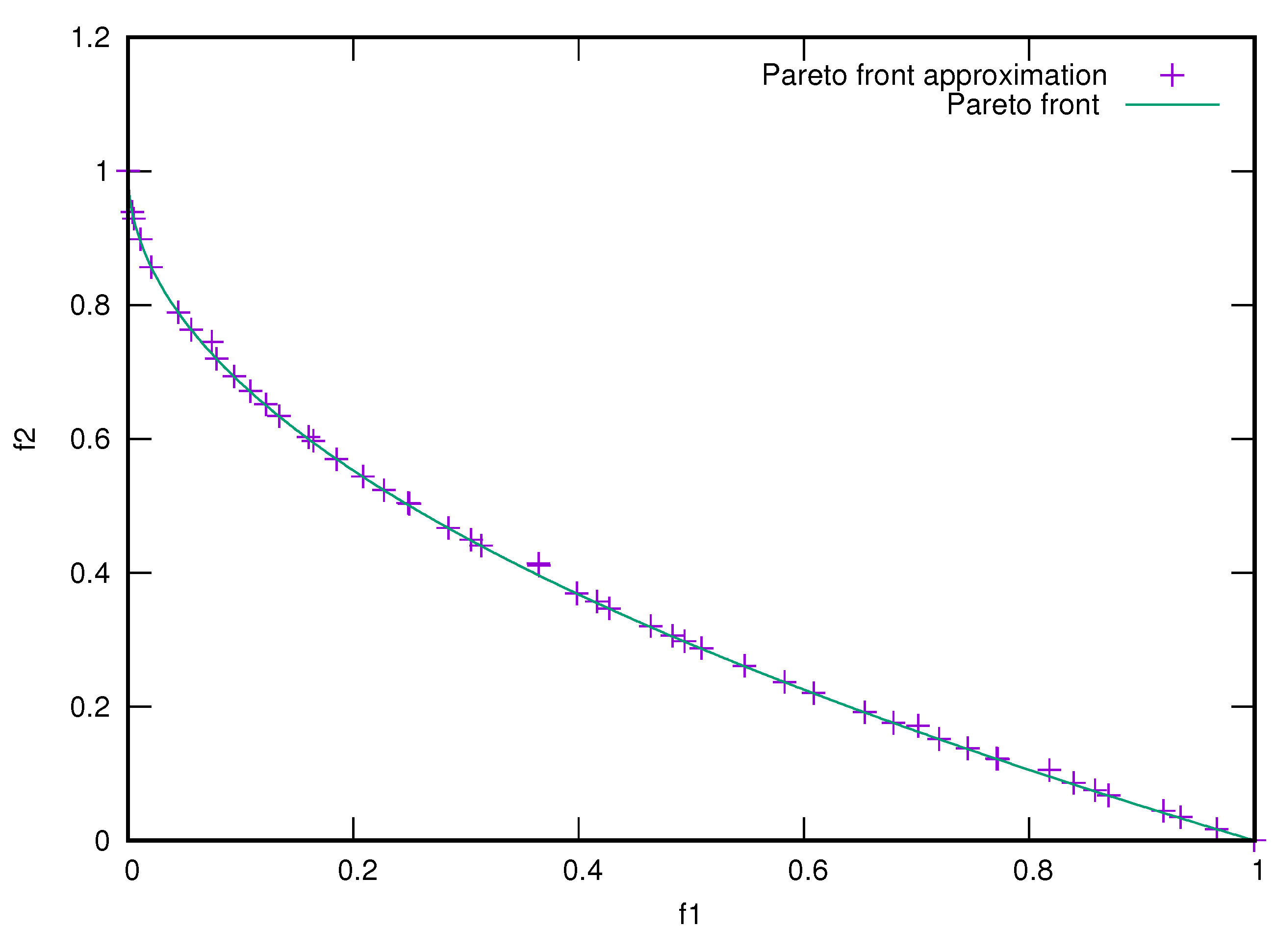
The concept of Pareto front approximation is illustrated in Figure 1, which includes the solutions found by an optimization algorithm when solving a multi-objective problem having two objective functions (named f1 and f2 in the figure). They are trade-off solutions in the sense that neither is better than the other in the two objectives. The true Pareto front in the example, depicted as a continuous line, has a convex shape and it can be observed that some of the obtained solutions do not completely overlap with the line (i.e., they have not fully converged to the Pareto front, so they are not optimal solutions) and the set of solutions covers all the Pareto front although it does not have a perfect spread out.

The most popular techniques to deal with multi-objective problems are metaheuristics [22], a family of non-exact, stochastic optimization algorithms which do not guarantee to find the optimum of a problem, but do usually provide high quality solutions (near optimal and sometimes optimal) within a reasonable amount of time and resources. There are different ways of classifying metaheuristics, one of which distinguishes between bioinspired (or nature-inspired) and non-bioinspired algorithms [6]. The first category is by far the most well known and used, including techniques such as evolutionary algorithms, particle swarm optimization, or ant colony optimization. The reference algorithm in multi-objective optimization, NSGA-II [7], is an evolutionary algorithm.

A metaheuristic typically follows an iterative process in which a set of tentative solutions P is manipulated somehow by a number of variation operators, aiming at progressively generating better solutions, as shown in the pseudo-code in Algorithm 1. In the case of evolutionary algorithms, the solutions and the set P are named, respectively, individuals and population, and the variation operators are crossover and mutation. The new produced solutions are evaluated to compute their corresponding objective function values and they are used to update the population. The main loop of the algorithm is executed until a stopping condition is met.

Algorithm 1 Template of a metaheuristic.

1: Set control parameters  2: $P\left(0\right)\leftarrow$ GenerateInitialSolutions()  3: $t\leftarrow$ 0  4: Evaluate($P\left(0\right)$)  5: while not StoppingCriterion( ) do  6:   $Q\left(t\right)$← Variation($P\left(t\right)$)  7:   Evaluate($Q\left(t\right)$)  8:   $P(t+1)$← Update($P\left(t\right)$, $S\left(t\right)$)  9:   $t\leftarrow t+1$ 10: end while 11: Return $P\left(N\right)$

A reason for the popularity of metaheuristics is the development of software frameworks that provide algorithms that are representative of the state of the art plus benchmark problems and utilities for performance assessment [23]. As commented in the introduction, in this work we use jMetal, a Java-based framework for multi-objective optimization with metaheuristics.

3. Related Work

Since the last decade, the optimal parameter calibration of hydrologic models has been tackled with mono- and multi-objective metaheuristic algorithms, usually providing successful results for different approaches of decision variables and objective functions. In particular, two early surveys [2,3] outlined the importance of using bio-inspired multi-objective approaches, as they are specially adapted to work as black-box optimizers with capabilities to explore the search space generated for each problem river basin scenario and for several objectives at the same time. In this regard, an interesting proposal was presented in Reference [24], where a sensitivity analysis and automatic calibration of a rainfall–runoff NedborAfstromnings model (NAM)  [25] was carried out with nine decision variables to measure the quantitative and qualitative variation of results. In this work, an Elitist Non-dominated Sorting Differential Evolution (NSDE) [26] algorithm was used to optimize two objective functions consisting on Average Root Mean Squared-Error (RMSE) of peak and low flow Events.

In Reference [27], a strategy that combined the principles of multi-objective optimization and depth-based sampling was presented with the title of Multi-Objective Robust Parameter Estimation (MOROPE). This algorithm applied multi-objective optimization to identify non-dominated robust model parameter vectors for the calibration of a distributed hydrologic model with a focus on flood events in a small pre-alpine and fast responding catchment in Switzerland. A thorough comparison was conducted in Reference [28] with a series of popular multi-objective algorithms (Borg, AMALGAM, GDE3, NSGA-II, OMOPSO, and SPEA2) for the calibration of the HBV (Hydrologiska Byråns Vattenbalansavdelning) conceptual rainfall-runoff model [29] with 14 real-valued decision variables and considering four objective functions. In this study, Borg and OMOPSO obtained, in overall, the best performance for the tackled instances. Also in 2013, the work presented in Reference [30] was centered on a river basin according to the distributed hydrologic model HEC-HSM (Hydrologic Engineering Center - Hydrologic Modeling System, https://www.hec.usace.army.mil/), for which a number of 10 decision variables and 4 objectives were approached with a multi-objective particle swarm optimization algorithm.

More recently, several variable balancing approaches for the exploration and exploitation of the NSGA-II, in the automatic parameter calibration of a HYdrological MODel (HYMOD) were evaluated in Reference [31]. These balancing approaches were compared with traditional static balancing methods (the two values are fixed during optimization) in a benchmark hydrological calibration problem for the Leaf River (1950 km²) near Collins, Mississippi.

Another related study is found in Reference [32], where authors analyzed how adding daily Total Water Storage (dTWS) derived from the Gravity Recovery And Climate Experiment (GRACE) as extra observations, besides the traditionally used runoff data, improved the calibration of a conceptual hydrological model within the Danube River Basin. As calibration approach, four popular evolutionary optimization techniques (NSGA-II, MOPSO, PESA-II, SPEA2) were tested to calibrate the model. Results indicated that NSGA-II performed better than the other techniques for calibrating GR4J using GRACE dTWS and in situ runoff data.

A common aspect in all these works is the use of already existing multi-objective optimizers (NSGA-II, SPEA2, MOPSO, etc.) with well-known hydrologic models usually requiring large number of parameters (HBV, HEC-HSM, GRACE, etc.), trying to find the best performing algorithm. Our proposal differs not only in the definition of a novel hydrologic model (Qom), but also in how the calibration with metaheuristics is conducted. Instead of looking for a particular technique, we take the practical approach of combining the results of seven algorithms, configured with commonly used settings, with the idea of combining the best solutions provided by all of them.

4. Hydrologic Calibration Strategy

In this section, the complete calibration strategy of the hydrologic model is detailed. First, the Qom model is explained with the main parameters and formulations. Then, the model calibration is formulated as a multi-objective optimization problem, so its objective functions and constraints are defined. Finally, the optimization approach is described from the perspective of software and computational issues.

4.1. Qom Model

The Qom model considers moisture, evapotranspiration, surface stored water and infiltration, and percolation processes, that is, those actions that cause water storage in the soil. It is applicable to permeable and impermeable soils and it determines the runoff in three layers, two of them superficial (permeable and impervious soils) and one another of underground flow. In order to determine the outlet flows in a given place in the basin in response to rainfall, we separate the total volumes of rainfall into volumes of losses and excesses discreetly over time, simulating for excess water the way in which runoff occurs, considering the transit and delay in the basin.

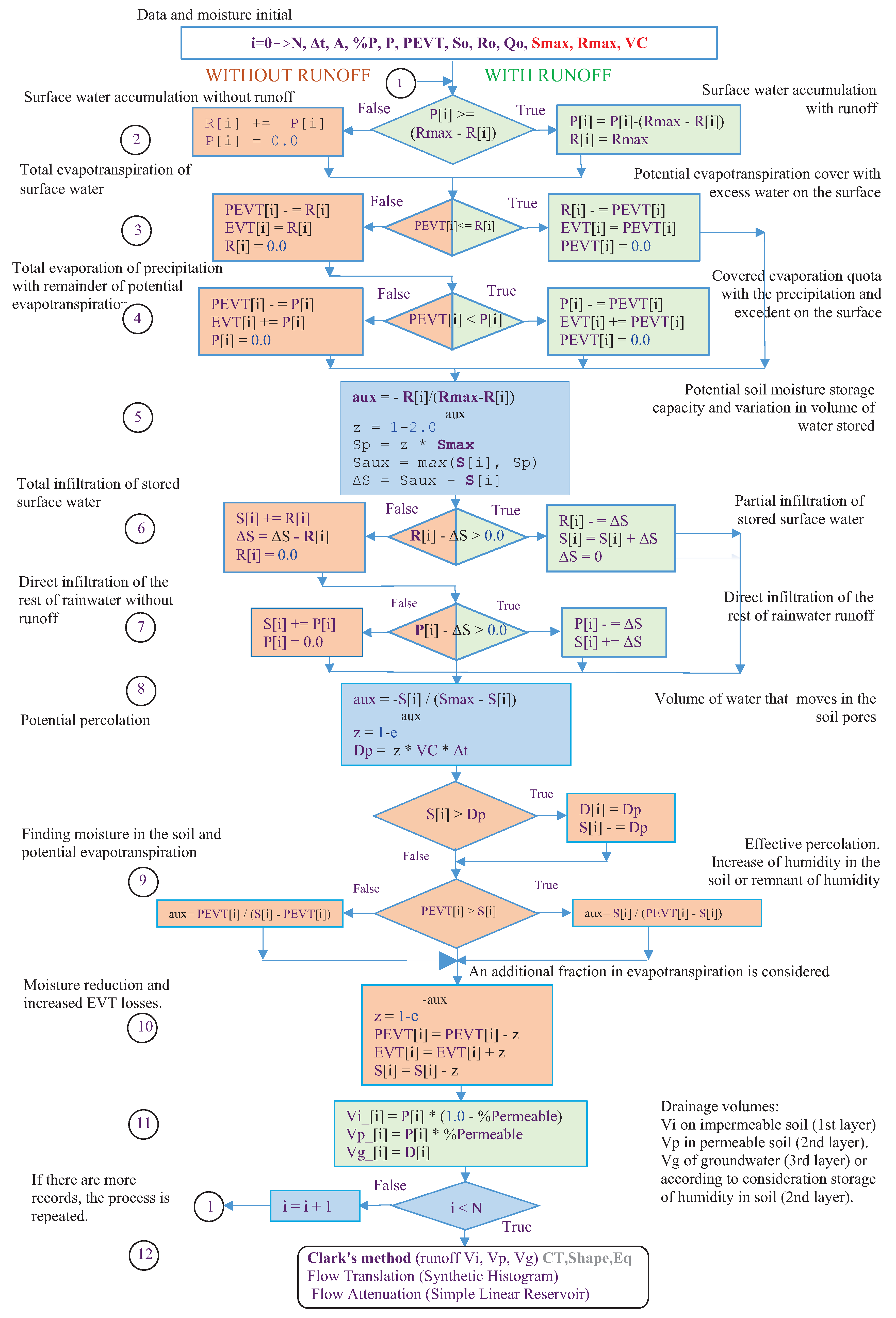
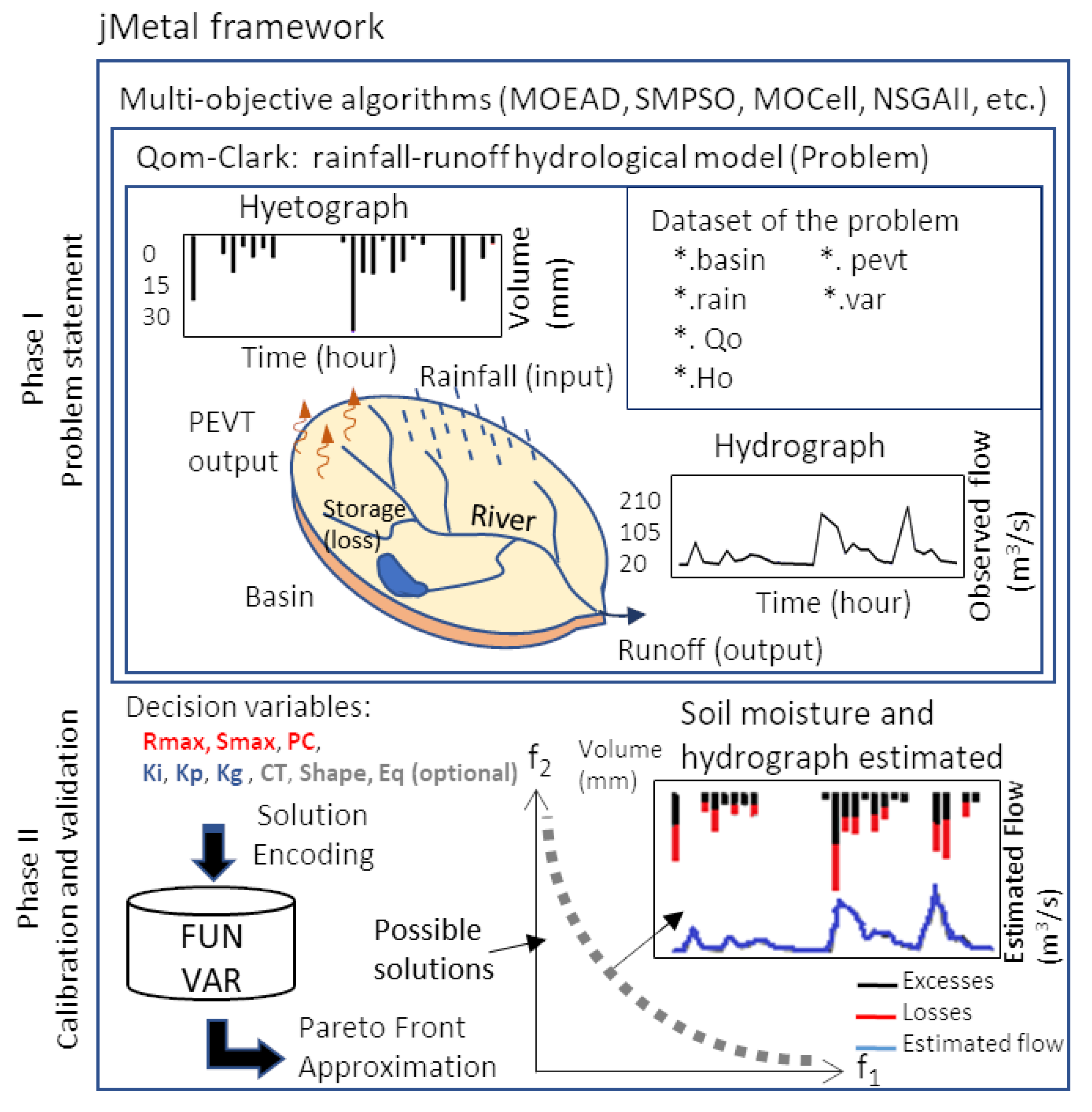
Therefore, besides the rainfall data and morphometric characteristics of the basin, the model needs three initial tuning parameters, namely the maximum storage water volume on surface $Rmax$, the maximum storage volume in the soil $Smax$ and the volumetric conductivity coefficient $VC$, which represents the volume of water that would move in three-dimensions in the soil towards the exit per unit of surface in a certain time, expressed in volume of water sheet per unit of time. These variables are emphasized in red color in the flow chart of Figure 2, which represents the mathematical model that corresponds to the equations commented in lines (1) to (12) of the this figure, involving the hydrologic natural processes of Qom. The computation cycle starts obtaining those required data from the problem specification given from the scenario instance, as well as the parameters (decision variables), to calculate the soil moisture states. A part of the rainfall defined with the variable P in the unity of the volume of the water sheet. Retentions in the basin are produced by surface depressions of the soil R, by the infiltration of water in the porosity of the soil S and percolates in permeable soils D. Another part of the volume is lost in the atmosphere through evaporation and plant transpiration $EVT$. The rest of the volumes would leave the basin superficially by a portion of impermeable areas $Vi$ and permeable ones $Vp$. In addition, another part $Vg$ of the volume can be percolated into deep layers remaining in the basin as soil moisture or as a mass of water that will be added to the underground outflow of the river.

When the Qom process is finished, the Vi, Vp and Vg volumes are passed to model the hydrograms. Clark’s model is then used for modeling direct runoff of watershed rainfall response. It is based on the concept that instantaneous unit hydrograph can be derived by routing the unit excess rainfall in the form of a time-area histogram (translation) through a single linear reservoir (attenuation). As a consequence of the application of this model, a new set of decision variables is taken into account for the calibration of the model, comprising: $Ki$, $Kp$, $Kg$ (emphasized in blue in Figure 3) and additionally the variables $CT$, $SC$ and $Eq$ can be enabled and considered (emphasized in grey); which leads to obtaining the solution vector $Qe$ that includes the estimated water flow as formalized in Equation (4).

$$Q{e}_i=Q{i}_i+Q{p}_i+Q{g}_i,1\le i\le N.$$

(4)

A description of all the terms and factors used in equations of Qom model can be found in

Table 1. Description of the terms in flowchart of Figure 2 and in Equations.

Term	Description
A	basin area (km${}^2$)
$Shape$	shape coefficient (dimensionless) +
$CT$	concentration time (h) +
$Eq$	other alternative exponetial base to $e=2.711828$ +
$\%p$	percent of pervious area
$\%i$	percent of impervious area
$Ro$	initial surface storage (mm)
$So$	initial soil storage (mm)
N	data register amount
$Rmax$	maximum surface storage (mm) *
$Smax$	maximum soil storage (mm) *
$VC$	volumetric conductivity coefficient (mm/h) *
i	vector register index
P	vector of precipitation, volume expressed in height (mm)
$\Delta t$	time step inter registers (s)
$PEVT$	vector potential evapotranspiration (mm)
R	vector of surface storage (mm)
$EVT$	vector of evapotranspiration (mm)
S	vector of soil storage (mm)
D	vector of percolated volume (mm)
z	percolation ratio between $Rmax$ and $R_i$ (dimensionless)
$z_2$	soil moisture ratio between $Smax$ and $S_i$ (dimensionless)
$Sp$	potential soil storage (mm)
$\Delta S$	soil moisture storage between the current state and the previous (mm)
$Dp$	percolated potential volume (mm)
$CR$	soil moisture by capillary rise (mm)
$Vi$	vector of runoff volume of impervious area (mm)
$Vp$	vector of runoff volume of pervious area (mm)
$Vg$	vector of percolated volume for losses or deep runoff (mm)
$Ki$	time delay for emptying reservoir Vi (h) ♯
$Kp$	time delay for emptying reservoir Vp (h) ♯
$Kg$	time delay for emptying reservoir Vg (h) ♯
$Qo$	vector of observed output streamflow (m${}^3$/s)
$Qe$	vector of estimated output streamflow (m${}^3$/s)
$Qs$	initial superficial streamflow (m${}^3$/s)
$Qd$	initial river base streamflow (m${}^3$/s)
$Qm$	average output streamflow observed (m${}^3$/s)
O	vector of observed data
E	vector of estimated solution

sign: * optimizing variables of Qom, ♯ optimizing variables of Clark, + optional decision variables.

. The coding of the solution consists of a real value vector that includes each decision variable as a parameter for calibration, three decision variables namely: $Rmax$, $Smax$ and $VC$, which represent the soil moisture estimated by Qom. Finally, in order to estimate the output flow Qe through Clark, we need 3 other decision variables: $Ki$, $Kp$, $Kg$, alternatively CT, Shape, Eq. Actual data values $Qo$ and those estimated by the computation of $Qe$ are used to calculate prediction errors in the two objective functions that will be optimized, as explained next.

4.2. Multi-Objective Formulation

To measure the quality of solutions obtained thorough the optimization process, a widely used statistic metric in hydrology is the Nash-Sutcliffe Efficiency coefficient ($NSE$) [33], which is computed by means of Equation (5). It is a normalized metric that determines the relative magnitude of the residual variance compared to the measured data variance, evaluating the model fit primarily during high-flow periods. $NSE$ ranges between $-\infty$ and $1.0$, with $NSE=1.0$ being the optimal value. Values between $0.0$ and $1.0$ are generally viewed as acceptable levels of performance, whereas values $<0.0$ indicate that the mean observed value is a better predictor than the simulated one, hence leading to unacceptable performance.

Based on this standard measure, our multi-objective approach is focused on minimizing two objective functions $f_1$ and $f_2$, by taking into account the time-series data from both, observed and estimated water flows in a given hydrologic scenario. The first objective function is based on $NSE$, although using the formulation $f_1=1-NSE$, to promote minimization (optimum in $0.0$, jMetal assumes that all the objective functions are to be minimized.) The second objective function is based on the percent bias ($PBIAS$) [34], which is formulated as $f_2=Abs\left(PBIAS\right)$ and measures the average tendency of the estimated data to be larger or smaller than their observed counterparts. $PBIAS$ is calculated as shown in Equation (6), with optimum value in $0.0$. Low-magnitude, positive, and negative values indicate, respectively, accurate model estimation, model underestimation bias and model overestimation bias.

$$NSE=1-\frac{{\sum }_{i=1}^N{(Q{e}_i-Q{o}_i)}^2}{{\sum }_{i=1}^N{(Q{o}_i-Qm)}^2}$$

(5)

$$PBIAS=\frac{{\sum }_{i=1}^N(Q{e}_i-Q{o}_i)}{{\sum }_{i=1}^{N}Q{o}_i.}$$

(6)

The problem formulation includes constraints based on the relative error in terms of the percentages $RE$, with $AE$ being the absolute error between observed and estimated values according to Equation (7). A constraint considers the mass balance function $MB$ (water balance or soil moisture accounting) that measures the river basin drainage with Equation (8) [UNESCO, 1971] for bounding the relative error $MBRE$. Other two constraints are defined for bounding the fitting errors in hyetograms as well as in losses and excesses volumes. In this work, solutions are constrained to $f_1<=0.3$, $f_2<=0.3$ and $MBRE<=0.3$ ($30\%$).

$$RE=\frac{AE}{O}beingAE=O-E$$

(7)

$$MB=\frac{(P-EVT-R-S-D)}{\Delta t}+(Qs+Qd)-Qe\pm AE=0.$$

(8)

4.3. Optimization Approach

Once we have formulated the calibration of the Qom model as a multi-objective optimization problem, the next step is to solve it to find an accurate approximation of the Pareto front and then take from it that solution providing the best overall result. Determining the best metaheuristic for a given problem instance is far from being a trivial process; thus, the No Free Lunch Theorem [35] states that all optimization algorithms that search for a particular problem of a class perform the same when averaged over all the problems in the class.

The experimental methodology we follow is not aimed at finding or designing a particular metaheuristic for the automatic calibration of Qom, but to make use of a set of existing algorithms and use all of them to get a Pareto front approximation. We want to avoid spending time in tuning the control parameters of the algorithms, so they will be configured with standard settings. Our approach is based on the assumption that each algorithm can efficiently explore a particular region of the search space, so running all of them independently and joining the results they provide is likely to yield a satisfactory set of solutions. To this end, we have selected a set of representative multi-objective metaheuristics which are included in the jMetal framework, namely: NSGAII [7], OMOPSO [8], SMS-EMOA [9], MOEA/D [10], AbYSS [11], SMPSO [12] and MOCell [13].

The scheme we follow is illustrated in Figure 3. The starting point is, for each riven basin, a dataset comprising 5 data files. A file with extension *.basin contains morphometric features with static parameters to characterize it, such as area, shape, percentage of permeable area $\%p$, initial surface and soil moisture ($Ro$ and $So$, respectively), start and end dates of analysis, time slot between registers $\Delta t$, and so forth. File *.var includes decision variables representing calibration parameters, as well as upper and lower bounds for algorithmic search. Information about total precipitations P is set in file *.rain, output flow data $Qo$ are in file with extension *.Qo and potential evapotranspiration data $PEVT$ are in file *.pevt. These files register observed data for each time period $\Delta t$. For each river basin, a problem instance is defined according to two or more series of data. One of these series is used for multi-objective optimization (calibration) and the remaining ones are used for validation, with regards to optimized solutions.

All the used algorithms are configured to find a bounded set of solutions after performing a maximum number of evaluations over the problem calibration data. When they finish, the results are stored in two files, named VAR and FUN, which contain, respectively, the found solutions (i.e., the values of the decision variables) and the corresponding Pareto front approximation (i.e., the objective function values). A number of 30 independent runs for configuration have been executed, and all the solutions produced by all the algorithms have been joined, so after removing the dominated solutions a set of non-dominated solutions is obtained. This set is used as a reference front.

After the optimization process, the next step is the decision making, consisting in the selection of one solution in the reference front that will allow the expert to compute an optimized prediction of the soil moisture state, volumes of looses and excesses and hydrographs. This step is described in the next section.

5. Experimentation

In this section, we first describe the scenarios used for validating our model. In particular, we have taken six problem instances involving river basins in Spain, USA, Brazil and Argentina. One of the goals of our proposal is to make it applicable to a wide range of scenarios. For that reason, the model has been tested with a number of river basins with different features of topography, land use in the region, and weather conditions. Then we detail the strategy followed to select a solution from the reference front obtained in the optimization phase. Finally, we analyze the results obtained when the model is configured with certain solution values selected (decision variables) and it is applied to the problem instances.

5.1. Problem Instances

Next we describe the river basin problems, including information about the datasets (a description of the main features of the river basins is included in Appendix A):

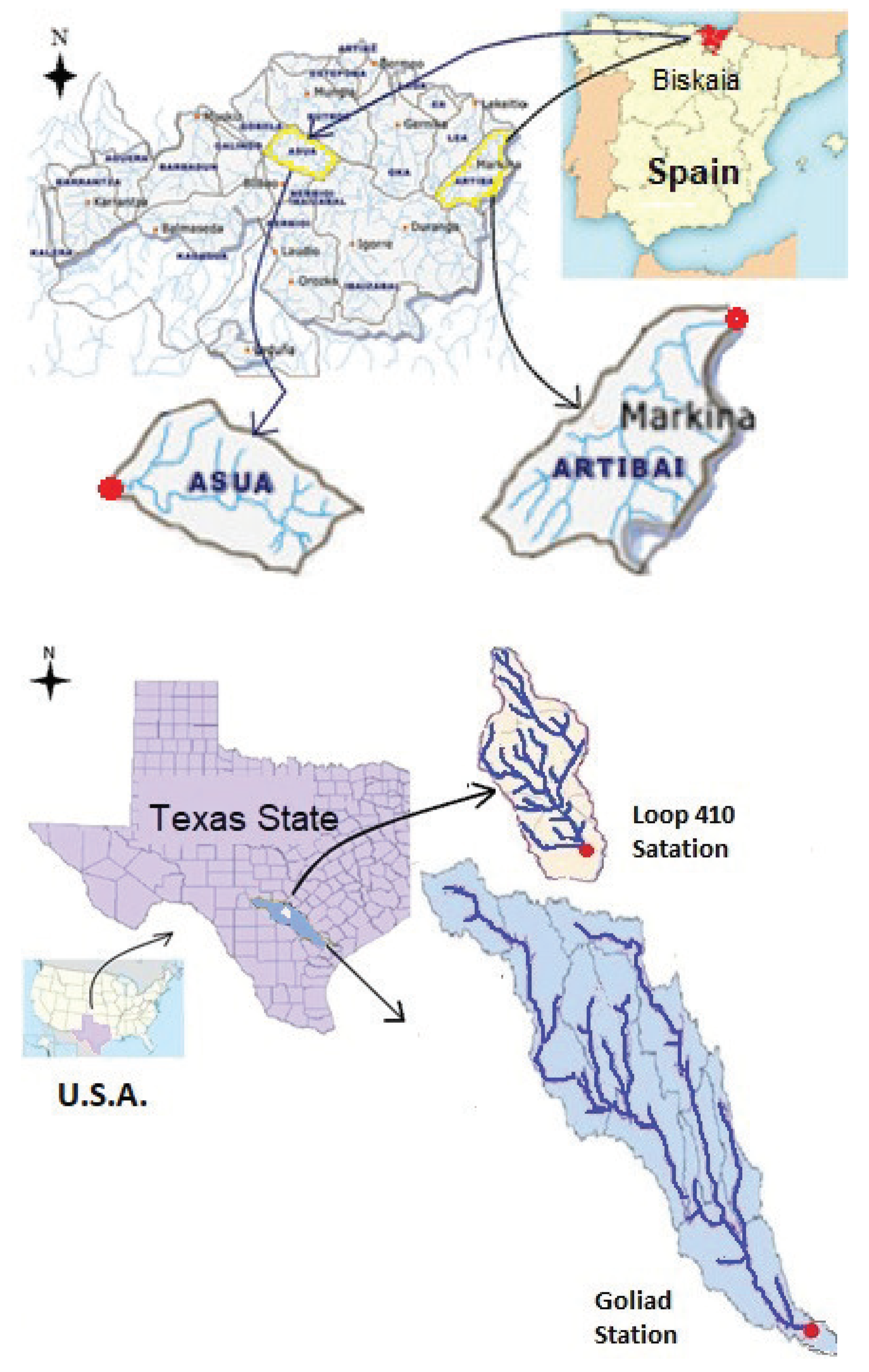
• Asua river basin, Bizkaia, Spain (73.44 km${}^2$, ${\Delta }_t$ = 24 h). The time period of registered data comprises from 6 June 2005 to 30 September 2009 and required the split in 4 different series due to the discontinuity of these data. Therefore, one of these subsets was used for model calibration, while the other three were employed for validation as independent test sets. These validation data sum up 2462 registries and they are annotated as continuous samples with time slot ${\Delta }_t$ = 24 h.
• Artibai river basin, Bizkaia, Spain (94.5 km${}^2$, ${\Delta }_t=10$ min). For this basin, the data registered comprise a time period from 17 June 2002 to 8 January 2004. Similarly to the previous instance, the whole dataset was split into 4 series of discontinuous data, one of them for calibration and the other three for validation, summing up 2462 continuous samples, although with time slot ${\Delta }_t$ = 10 min.
• San Antonio river sub-basin, station Loop 410, Texas, USA (323.7 km${}^2$, ${\Delta }_t=15$ min). Prior dry periods and two continuous events that generated two crescent peaks were used for calibration, with 500 records corresponding to a total of 94,538 records that included two data series for validation. The time period for calibration data was from 15 November 2010 to 18 November 2010, with ${\Delta }_t$ = 15 min, while the two validation periods comprised data from 17 November 2009 to 26 July 2012 and from 4 June 2013 to 24 March 2016, both with ${\Delta }_t$ = 15 min.
• San Antonio river basin, station Goliad, Texas, USA (10,000 km${}^2$, ${\Delta }_t=24$ h). In this instance, hydrometric data are registered with ${\Delta }_t$ = 24 h. Each test corresponds to a single event, comprising the most severe storms that developed in the region to the date considered in the study.
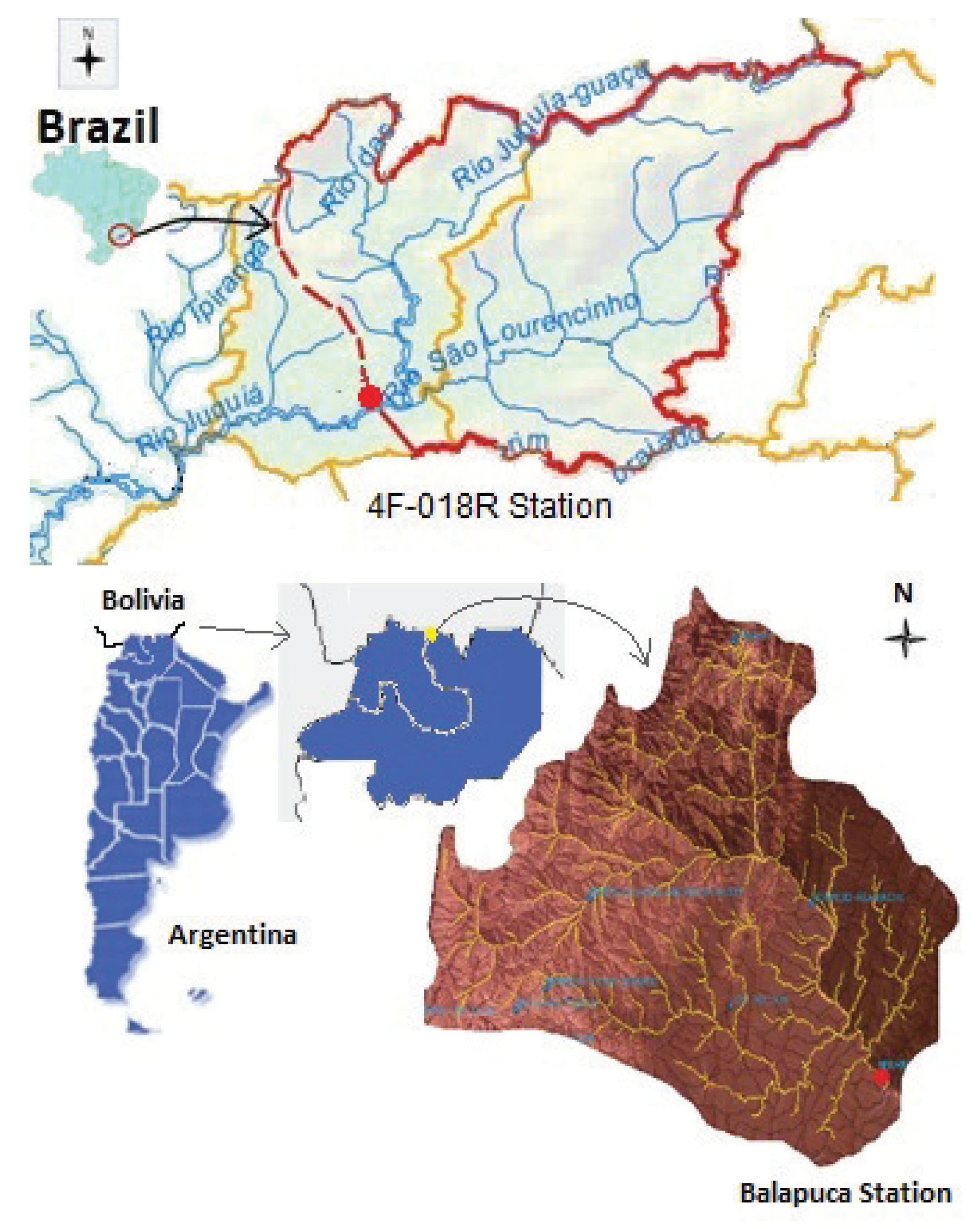
• Juquiá river basin, station 4F-018R, São Pablo, Brazil (4.360 km${}^2$, ${\Delta }_t=15$ min). Due to the temporary discontinuity of the data and the time difference between series of records, this sub-basin dataset was split into four parts, two for periods with ${\Delta }_t$ = 1 h and other two for periods with ${\Delta }_t$ = 15 min. It is worth noting that calibration was made including several hard events with different time scales of 1 h and 15 min, although keeping a single set of the same parameters.
• Upper Bermejo river basin, station Balapuca, Argentina-Bolivia (4398.8 km${}^2$, ${\Delta }_t$ = 24 h). For calibration, a period of several events was used between 2 December 1971 and 1 January 1972 comprising 412 days. For validation, one of the longest continuous series was used in this study, with dates from 2 January 1972 to 1 September 2015 including 15,766 records. Accumulating a total precipitated volume of 56,902 mm.

The data of two first instances (1 and 2) were obtained from the Bizkaiko Foru Aldundia, Diputación Foral de Bizkaia (BFA-DFB) through the website of this regional Spanish organism (http://web.bizkaia.net). The morphometric features were obtained from Reference [36]. Problem instances 3 and 4 from Texas State (USA) correspond to drainage areas at Loop 410 station (sub basin ID 08178565) and Goliad station (sub basin ID 08188500) and morphometric features from Reference [37]. Meteorologic data used for these two instances were taken from the United States Geological Survey (USGS) (http://nwis.waterdata.usgs.gov/nwis). The data on instance 5 were obtained from Agência Nacional de Águas (ANA), Brazil (https://www.ana.gov.br/eng/featured/monitoring-1/monitoring). Finally, data on instance 6 were obtained from the Bermejo River National Commission (COREBE) (http://corebe.org.ar/web2015/informacion-hidrologica/).

Problem instances and their data subseries were identified by an alphanumeric code of 4 characters. The first number in this code indicates the river basin with specific morphometric features; the second number (separated with dot) is the data series of different time periods; the third character could be “C” to indicate continuous samples with several storming events or “S” meaning a single event (one storm); the fourth character could be “C” to indicate this series is used for calibration (optimization) or “V” to specify the data series is used for validation as external test set. For example, instance 1.1CC corresponds to Asua river basin data series 1 with continuous samples that are used for calibration.

5.2. Solution Selection Strategy

As commented before, the results of optimizing each problem with the seven multi-objective metaheuristics constitute a reference front composed of the non-dominated solutions produced by all the algorithms. Now, we proceed to describe and apply a solution strategy to select from the reference front that solution providing the best trade-off, according to the two objective functions, to properly set the Qom model with a high accurate prediction capability.

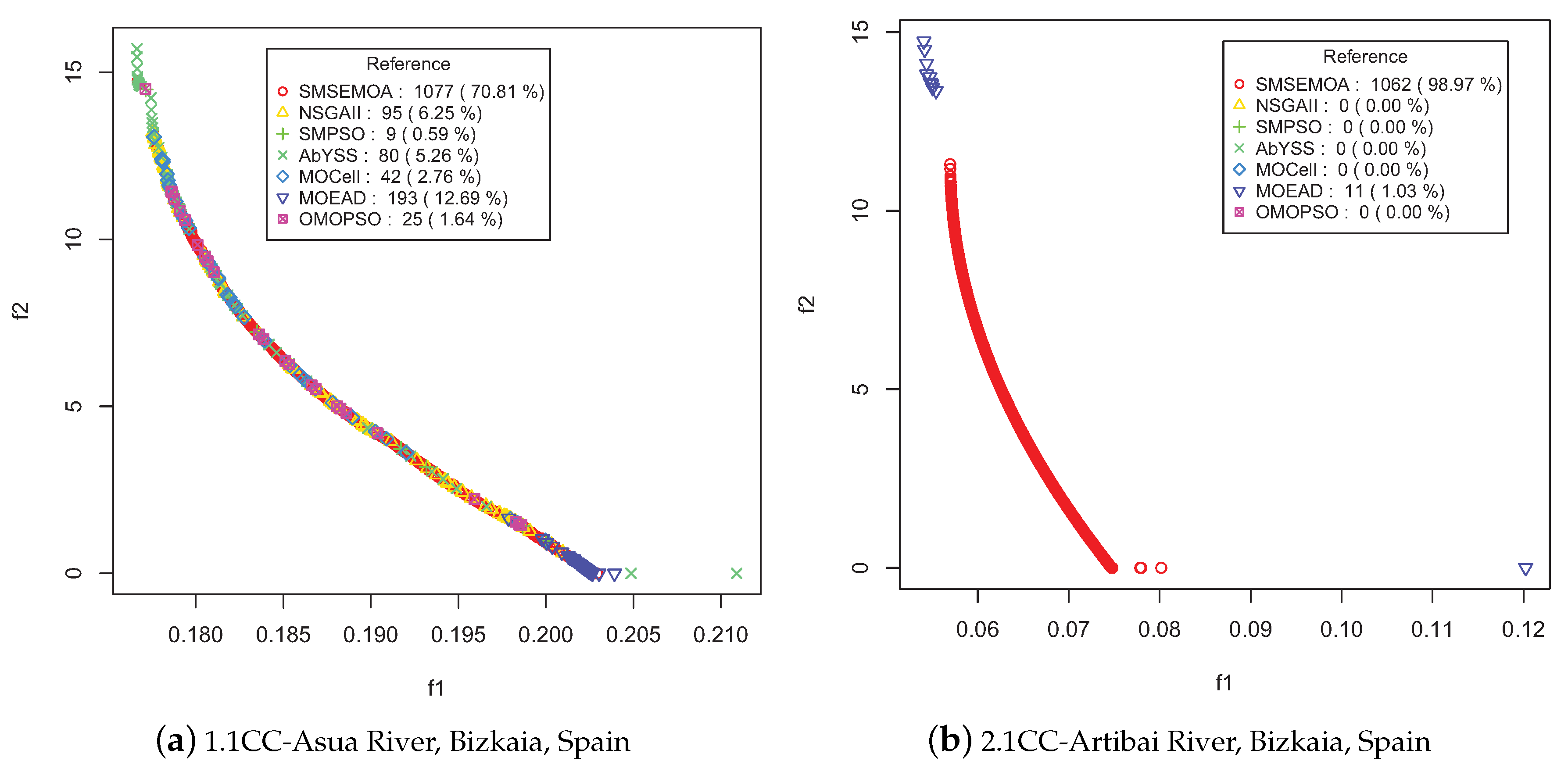
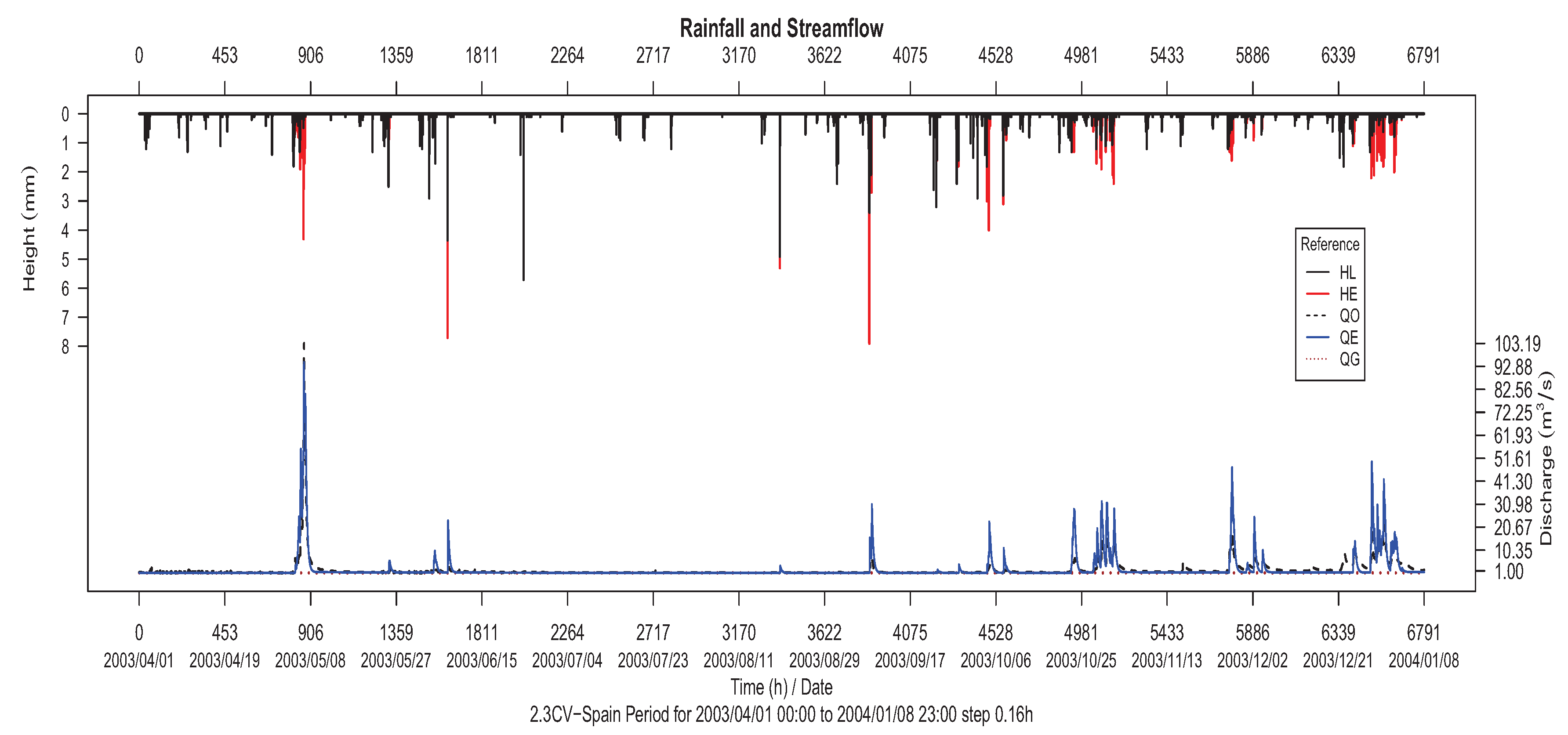
Figure 4a,b show the reference fronts obtained for problem instances 1 and 2, respectively, including information about the number and percentage of solutions contributed by each algorithm to the reference front. We use a different combination of symbols and colors for each solution to associate to the algorithm that produced it.

We start by analyzing the Asua river basin (a) with calibration series 1.1CC. We observe that all the algorithms have contributed to the reference front, with SMS-EMOA being the one contributing with more solutions by far (70.81%), followed by MOEA/D (12.69%), NSGA-II (6.25%), AbYSS (5.26%), MOCell (2.76%), OMOPSO (1.64%), and SMPSO (0.58%). However, it is worth noting that the solutions in the extreme regions of the reference front have been obtained by algorithm AbYSS (green points with symbol ×). We observe also that the solutions of MOEA/D (blue points with symbol ▿) are concentrated on the bottom part of the front, which corresponds to higher values of the first objective (NSE) and lower values of the second objective function (PBIAS). The interesting fact is that all the algorithms complement each other, as the reference front has no gaps.

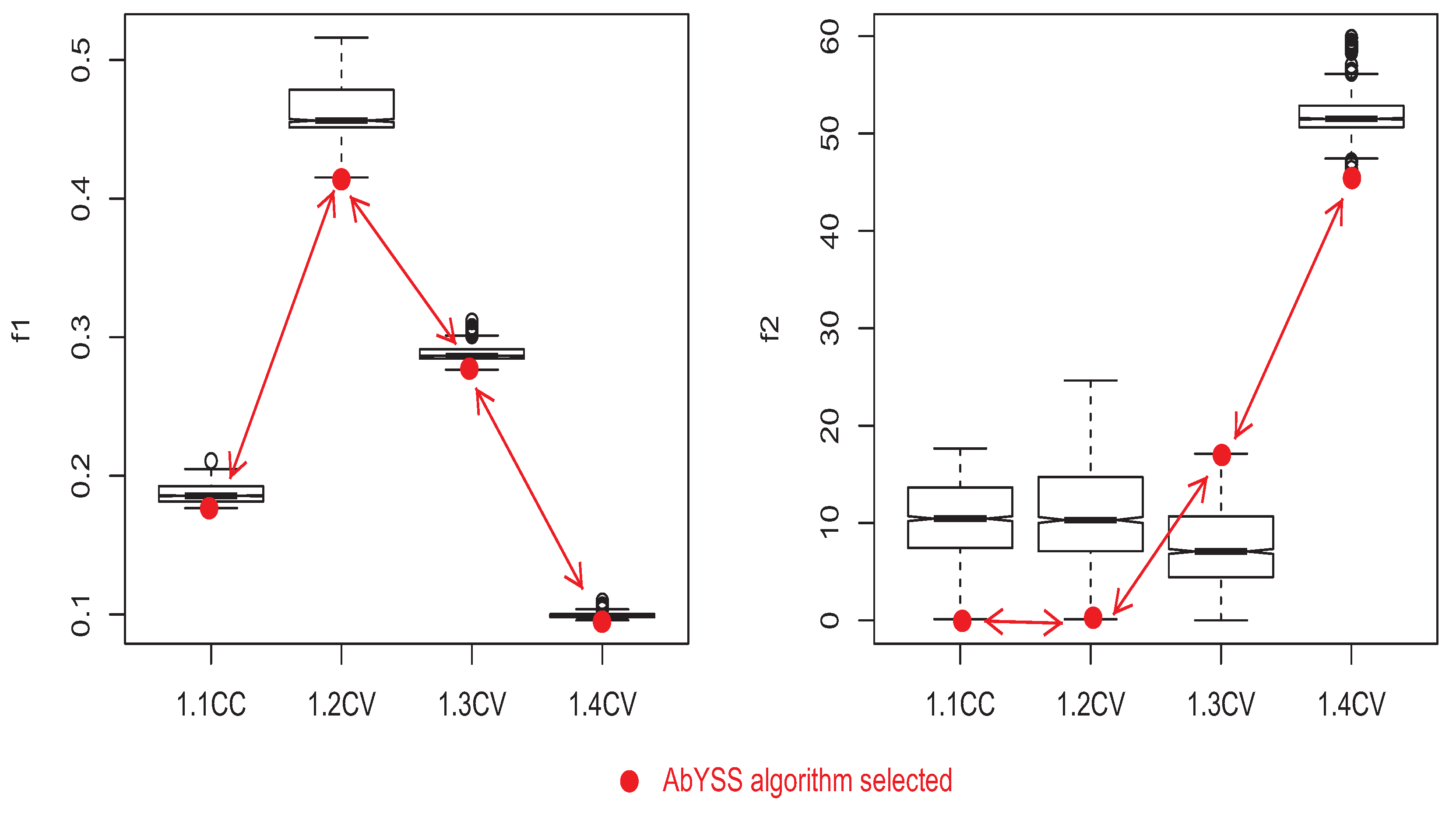
We focus now on the numerical dispersion of results obtained for the calibration series with regards to validation ones on the Asua river data. Figure 5 includes the boxplots of distribution of results for each objective function and four data series of the problem. We observe that there are not high differences between calibration and validation. For objective function f1 (1-NSE measure), quarterlies of series 1.1CC, 1.3CV and 1.4CV are in the range of 0.9 and 0.7 (NSE = 1 − f1) and only 1.2CV shows higher dispersion with quarterlies 0.57 and 0.47, but without outliers. These results are classified in the reference literature [38] from very good to excellent. In the case of PBIAS (f2), series 1.1CC, 1.2CV and 1.3CV show predicted results between 0% and 25% also without outliers, whereas for validation series 1.4CV, results alternate from 45% to 60%, but with low dispersion between maximum and minimum limits. As AbYSS yielded the extreme solutions in the calibration, we have outlined the solutions having the lowest values for the two objectives in both, the calibration and validation results. We observe that AbYSS also gets the lowest values in all the cases but one, the 1.3CV dataset with the second objective function.

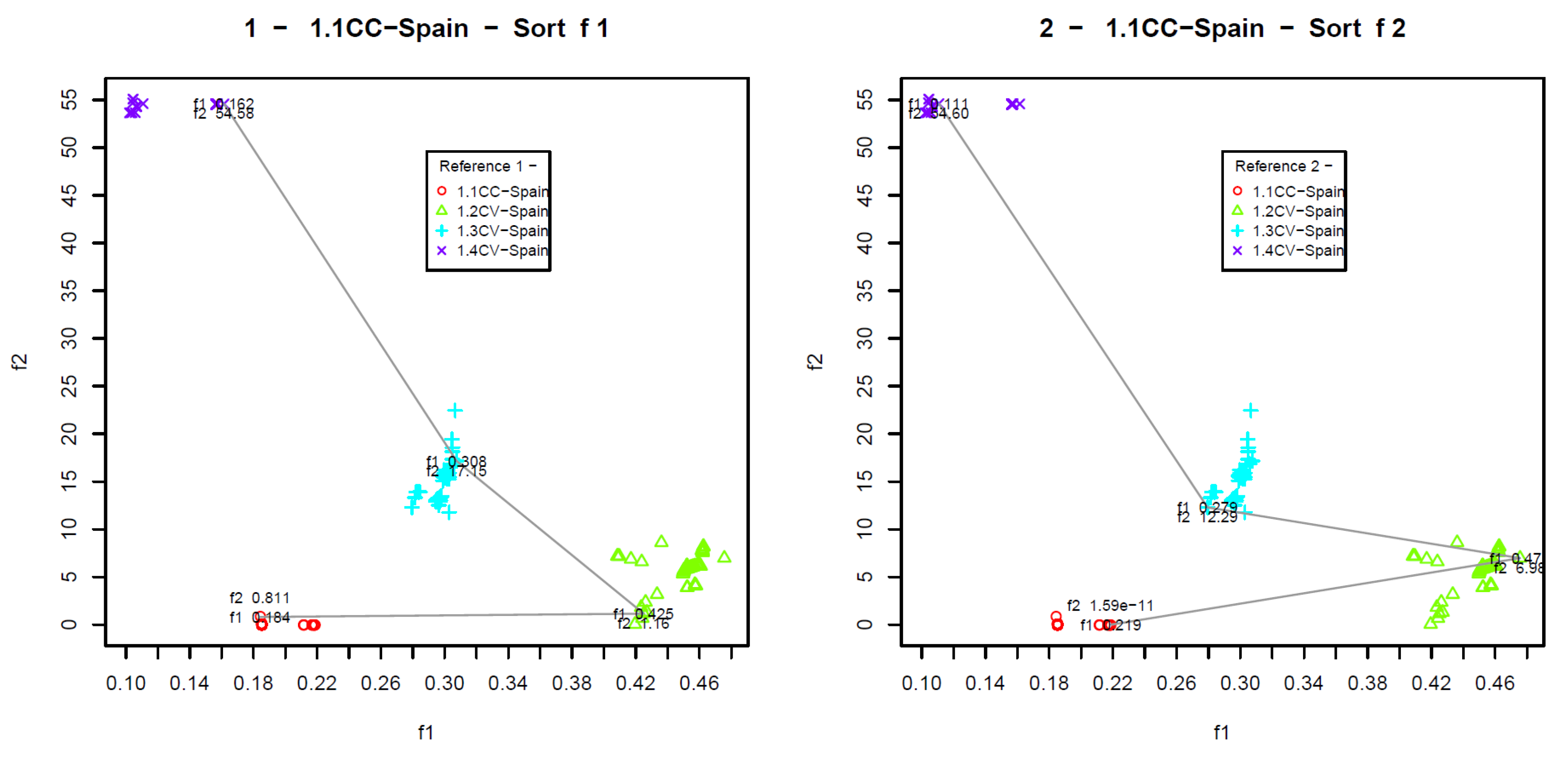
Keeping this in mind, we can now plot the different prediction error distributions of the two objective function values (1-NSE versus PBIAS), to show the influence of calibrated variables when applied to validation data series. This way, as shown in Figure 6 for problem instance 1 (Asua river basin), calibrated solutions remain accurate when applied to the corresponding validation data, although better results are obtained in general when selecting the best solution in 1.1CC according to f2 (Figure 6 right). It can be argued that, for this specific problem instance, we can select the vector of decision variables (solution) that sets the Qom model with higher precision for three validation series. This strategy has been followed for all the problem instances worked in this study with similar results, hence making the solution selection easier in the decision making process.

We now analyze instance 2 (Artivai river basin) for series 2.1CC, the reference front of which is plotted in Figure 4b. In this case, SMS-EMOA is again the multi-objective calibrator with a higher percentage of solutions contributing to this front approximation with 98.97% and also with low dispersion in objective functions (variation of $f1\in [0,0.08]$). However, according to the previous strategy, after validation of series 2.1CV the most accurate solution is provided by MOEA/D, which only contributes with 1.03% to the reference front. 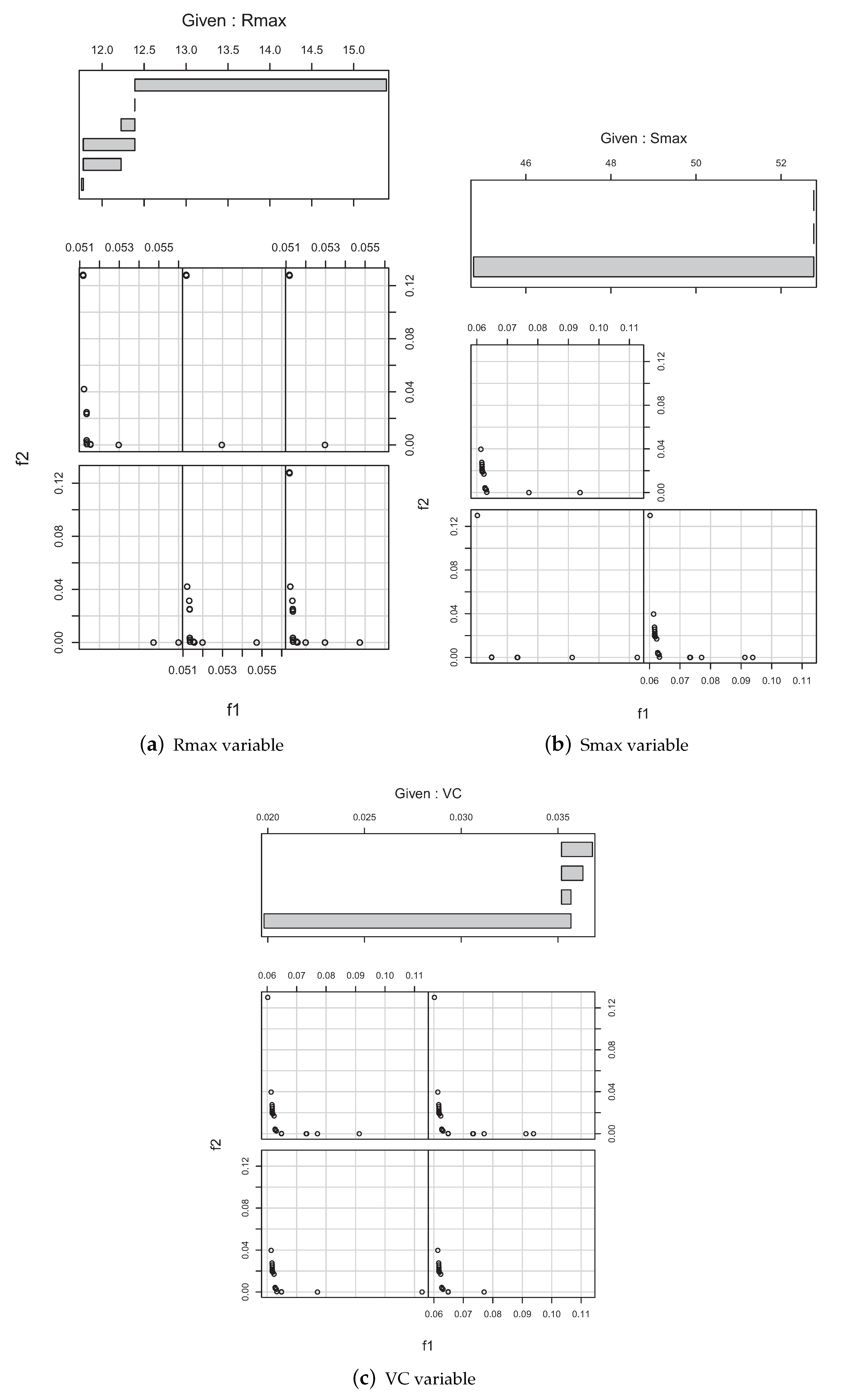This is an interesting result that can be explained by checking decision variables $Rmax$, $Smax$ and $VC$, as shown in Figure 7. In these graphs, the ranges of these two variables are plotted with regards to the corresponding solutions in the reference front, so for SMS-EMOA they do not exceed a value of 0.5 mm. Conversely, for MOEA/D solutions, the maximum values of $Rmax$ and $Smax$ are 3 mm and 30 mm, respectively. This way, the spectrum of accurate solutions is expanded to those located at the extremes of the reference front, as plotted in Figure 4b. This leads us to suggest that this solution selection strategy does not necessarily depend on a given outperforming algorithm (SMS-EMOA in this case), but on a validation methodology with an external series of data, that provide trade-off values in decision variables.

5.3. Results After Choosing Solutions

Once the resulting solutions are selected after calibration and validation, their corresponding decision variables are registered and analyzed in terms of the hyetographs and hydrograms, where the volumes of losses and excesses, as well as the fitting error of observed versus estimated data series are plotted. These decision variables are shown in

Table 2. Selected solutions from resulting RF approximations after experiments and validations.

Problem Instance	$\mathit{Rmax}$ (mm)	$\mathit{Smax}$ (mm)	$\mathit{VC}$ (mm/h)	${\mathit{K}}_{\mathit{i}}$ (h)	${\mathit{K}}_{\mathit{p}}$ (h)	${\mathit{K}}_{\mathit{g}}$ (h)
1. Asua River	16.0	131.0	0.09	8613.0	6.6	20,446.0
2. Artibai River	12.7	45.0	0.02	653.0	7.6	75,596.0
3. San Antonio River, Loop 410	13.7	46.0	0.29	132.0	1.1	3.0 × 10${}^6$
4. San Antonio River, Goliad	218.0	435.0	0.29	107.0	50.0	16,150.0
5. Juquiá River, 4F-018R	7.0	10.0	0.01	50.0	4500.0	3000.0
6. Bermejo River, Balapuca	17.0	349.0	0.27	1829	60.0	50,398.0

for each problem instance, which have been used to set the Qom model.

The corresponding NSE and PBIAS obtained by using these variables on the different calibration and validation data series are shown in

Table 3. Objective values NSE and PBIAS of selected solutions according to each data series, time period, and registry.

Problem Instance	Data Series	Time Period	# Registries	NSE	PBIAS
1 (Asua river)	1.1CC ${\Delta }_t$ = 24 h	05-02-2007:10-08-2007	187	0.82	8.7%
	1.2CV ${\Delta }_t$ = 24 h	06-06-2005:08-01-2007	582	0.56	9.4%
	1.3CV ${\Delta }_t$ = 24 h	09-09-2007:11-4-2009	581	0.75	9.4%
	1.4CV ${\Delta }_t$ = 24 h	08-06-2009:30-09-2009	115	0.82	18.0%
2 (Artibai river)	2.1CV ${\Delta }_t$ = 10 min	17-06-2002:31-12-2002	29,224	0.63	23.9%
	2.2CV ${\Delta }_t$ = 10 min	01-02-2003:04-03-2003	4588	0.68	0.5%
	2.3CV ${\Delta }_t$ = 10 min	01-04-2003:08-01-2004	40,747	0.53	12.8%
	2.4CC ${\Delta }_t$ = 10 min	17-06-2002:21-06-2002	637	0.85	22.3%
3 (San Antonio, Loop 410)	3.1CC ${\Delta }_t$ = 15 m	15-11-2010:21-12-2010	300	0.85	24.6%
	3.2CV ${\Delta }_t$ = 15 min	17-11-2009:12-06-2012	94,315	0.43	0.5%
	3.3CV ${\Delta }_t$ = 15 min	04-06-2013:24-03-2016	98,328	0.64	53.3%
4 (San Antonio, Goliad)	4.1SC ${\Delta }_t$ = 24 h	15-10-1998:02-11-1998	19	0.85	4.3%
	4.2SV ${\Delta }_t$ = 24 h	23-06-2002:31-08-2002	70	0.91	4.5%
	4.3SV ${\Delta }_t$ = 24 h	09-03-2007:09-03-2007	18	0.84	6.2%
5 (Juquiá, 4F-018R)	5.1CC ${\Delta }_t$ = 1 h	09-07-2005:09-07-2005	2,351	0.79	5.0%
	5.2CV ${\Delta }_t$ = 1 h	17-10-2005:04-01-2006	1634	0.40	3.7%
	5.3CV ${\Delta }_t$ = 15 min	01-05-2013:13-06-2013	3987	0.10	6.6%
	5.4CV ${\Delta }_t$ = 15 min	11-08-2013:22-12-2013	17,551	0.60	1.05%
6 (Bermejo river, Balapuca)	6.1CC ${\Delta }_t$ = 24 h	01-12-1971:02-07-1972	214	0.89	1.3%
	6.2CV ${\Delta }_t$ = 24 h	02-07-1972:31-08-2015	15,766	0.26	1.9%

, where additional information concerning the time period of observation, time slot of registration (10 min, 15 min, 1 h, and 24 h) and the number of registries is also provided. In general, values of NSE ≥ 0.75 and PBIAS ≤ 10% are obtained for calibration series, while NSE ≥ 0.6 and PBIAS ≤ 25% can be observed for validation series of data. In accordance with reference studies in the literature [39], where registration periods are conducted monthly, values of NSE ≥ 0.50 and PBIAS ≤ 25% can be considered as satisfactory. In the light of these results, we can claim that the prediction errors obtained by our proposed Qom model based on multi-objective calibration are more than satisfactory, since it is able to deal with complex problem instances with observation time periods significantly lower than 1 month, as done in Reference [39].

More in depth, when focusing on a specific solution for a river basin, a series of hydrologic results are extracted, which leads the expert to define a hydrology engineering project. An example of these values are shown in

Table 4. Hydrologic results for instance 6.2CV (Cuenca del Alta del Rio Bermejo, Argentina), Qom-Clark model for period 2 February 1971 09:00 to 3 April 2014 09:00 step 24.0 h.

Concept	Parameter	Volume
		(mm)	(Hm${}^3$)
Initial condition	Rain	80,544.35	354,300.07
	Superficial Storage	0.00	0.00
	Soil Storage	0.00	0.00
Qom solution	EVT	8855.45	38,953.54
	Superficial Storage	0.00	0.00
	Soil Storage	20.13	88.55
	Groundwater Runoff	47,329.02	208,191.81
	Superficial Runoff	24,339.74	107,066.15
	Total volume estimated	80,544.35	354,300.07
Balance AE	EVT	0.00	0.00
	Relative Error (RE)	0.00	-
Total Volume Runoff	In pervious superficial	-	96,359.53
	In impervious superficial	-	10,706.61
	Off growndwater	-	208,191.81
	Corff. Runofff	-	0.30
Comparison of water volumes	Observed hydrograph	28,287.22	124,430.37
	Estimated for Clark (RE = 2.05)	28,866.98	126,980.63
	Estimated for Qom (RE = −13.95)	24,339.74	107,066.15

and

Table 5. Specific hydrograph results for instance 6.2CV (Rio Bermejo, Argentina), Clark model for period 2 February 1971 09:00 to 3 April 2014 09:00 step 24.0 h.

Concept	Parameter	Streamflow (m${}^3$/s)
Hydrograph	Estimated	2726.94
	Superficial impervious	41.26
	Superficial pervious	2677.15
	Groundwater	17.58
Flow peak of Hydrograph	Observed maximum	3278.74
	Relative error max peak	−16.83
	Observed second	2464.00
	Relative error second max peak	10.67
Minimum flowrates	Observed	6.58
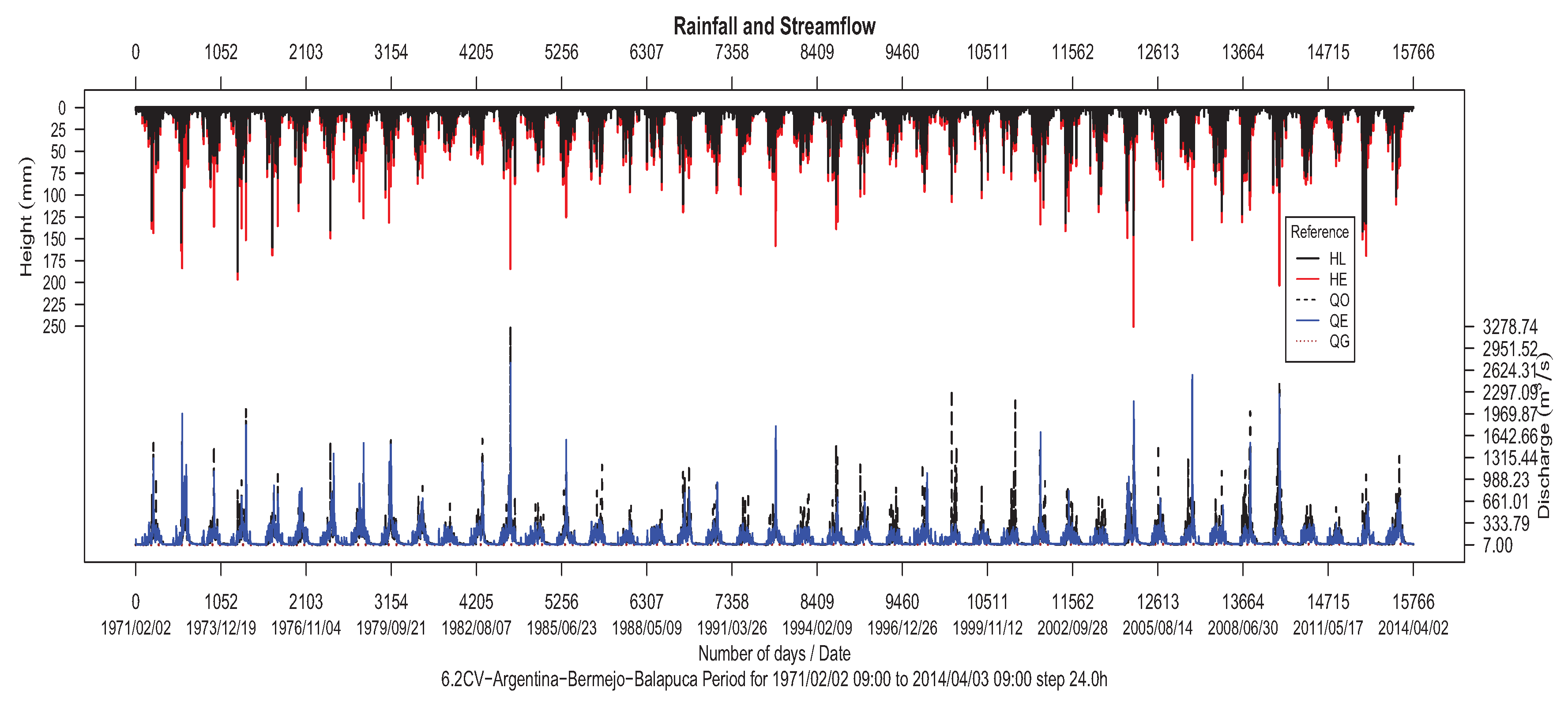
	Estimated	7.00

, which include the specific mass balance obtained by Qom-Clark and estimated peak values with relative errors for problem instance 6.2CV (Rio Bermejo, Argentina), and data period 1971 09:00 to 3 April 2014 09:00 step 24.0 h.

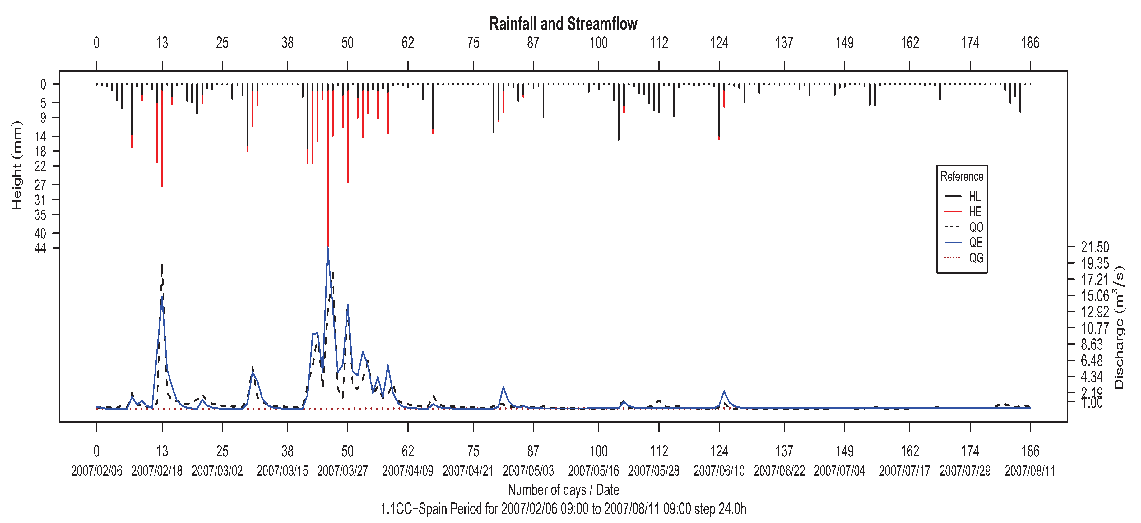
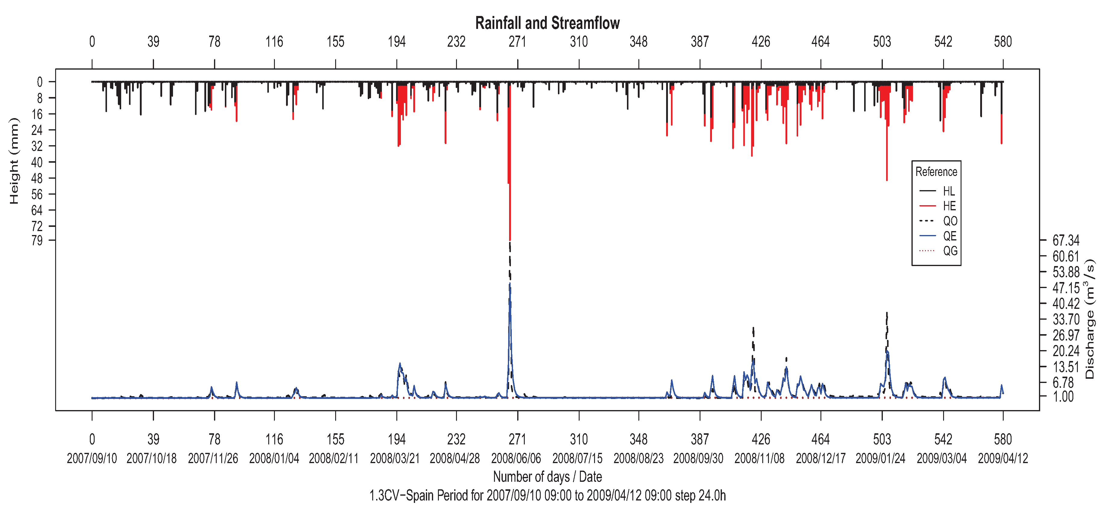
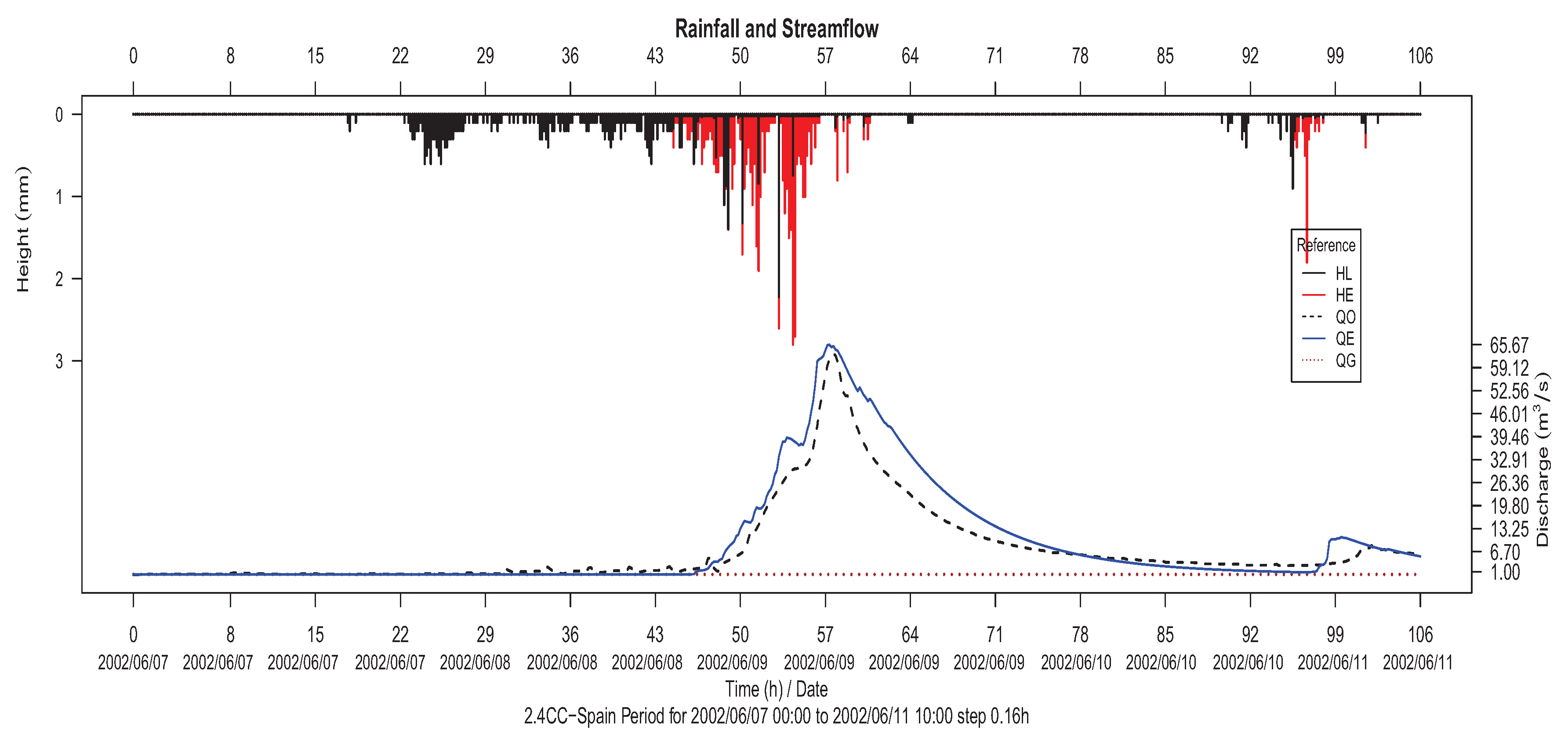
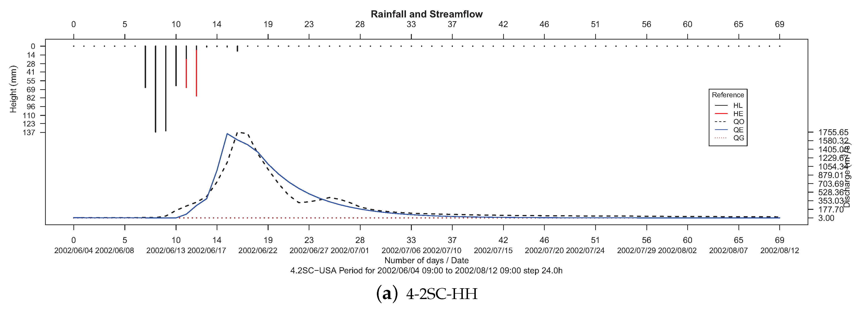
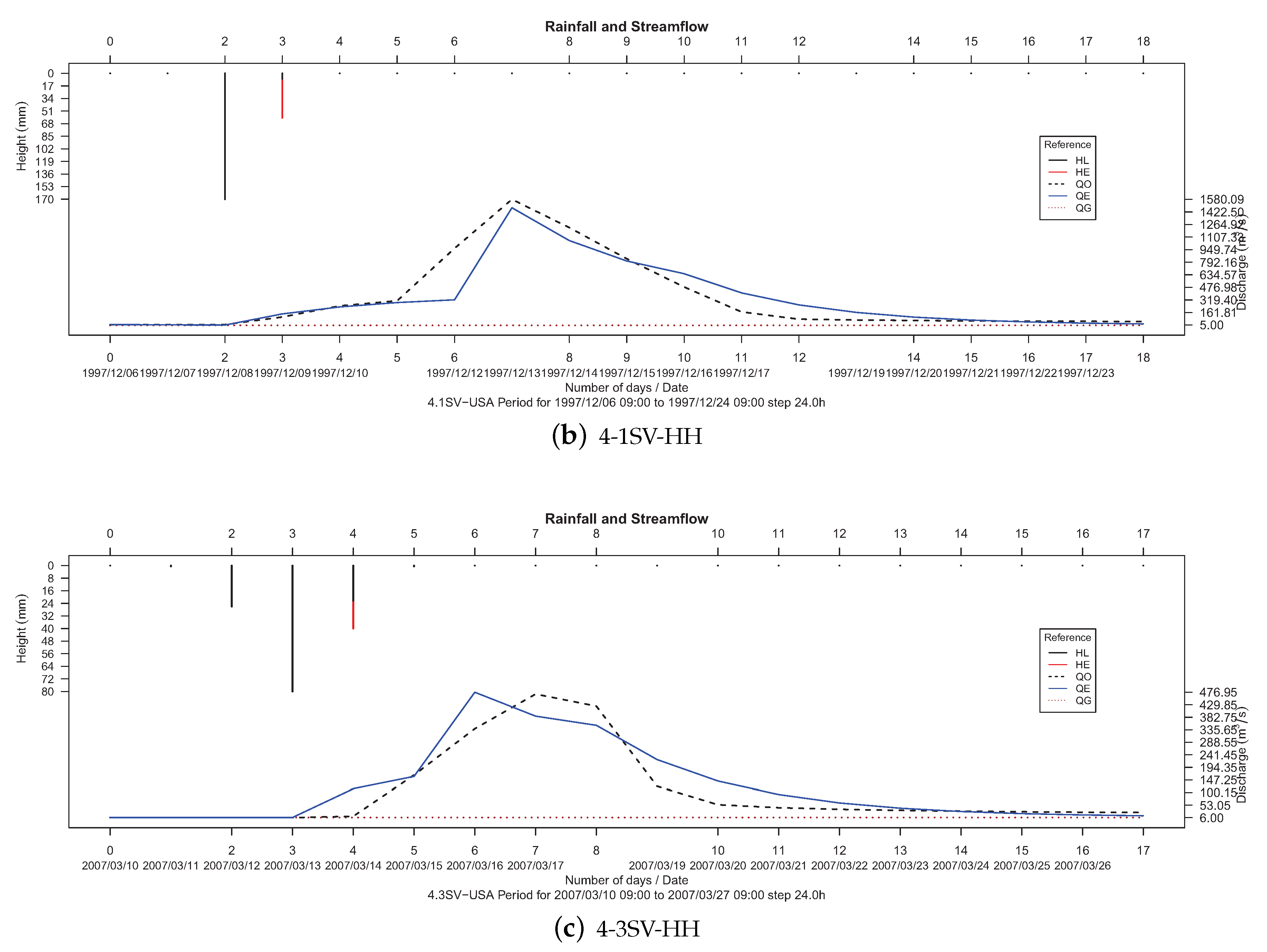
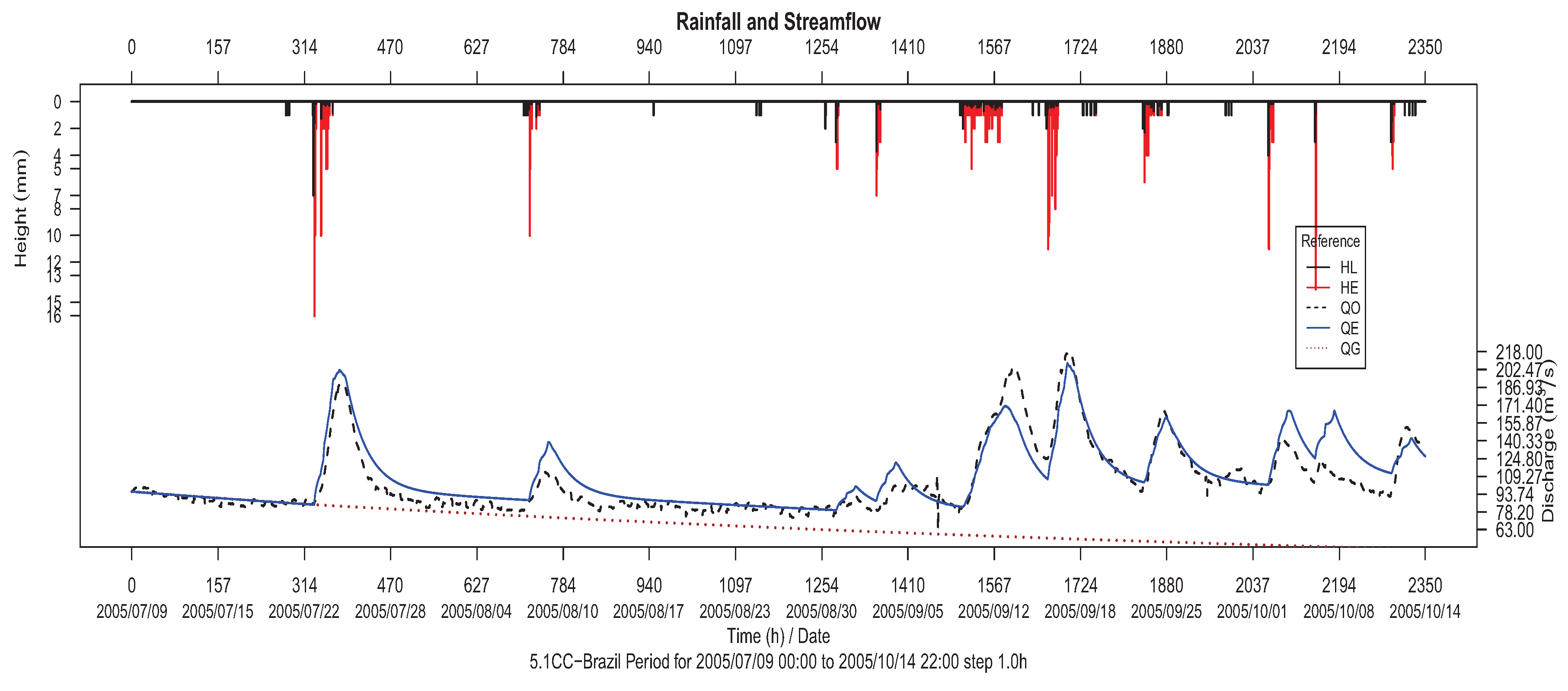
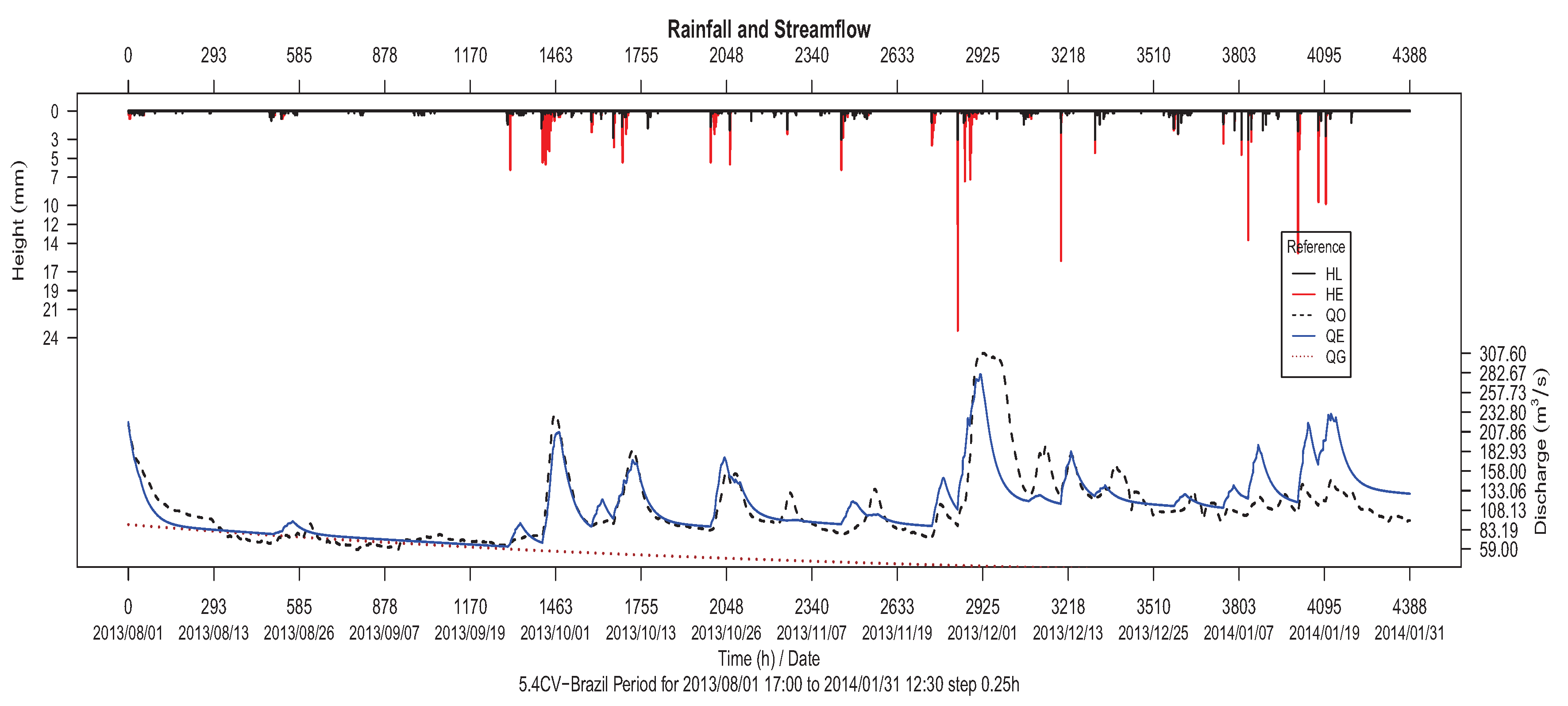
From a visual perspective, it is possible to check the quality of the hydrographic models obtained by plotting the hyetographs, which represent the humidity losses (HL) and excesses (HE) values from input data, together with the hydrographs, with observed (QO) and estimated (QE) outputs. In this way, Figure 8 shows the resulting rainfall and streamflow by means of the hyetograph and hydrograph of the 1.1CC (Asua river basin) calibration data series, where we can observe the high correspondence between water losses/excesses and the predicted series (estimated data), which indeed fits the curve of observed data. For validation data series 1.3CV, a similar plot is made in Figure 9 to better show the precision in estimated streamflow (QE), so even for external data (not used in calibration) a high prediction can be reached with the proposed approach.

A similar observation can be extracted from problem instance 2 (Artibai reiver basin), for which Figure 10 and Figure 11 show the corresponding hyetographs and hydrographs of calibration and validation. In this case, although the amount of data used for calibration is lower than for validation, the precision power of the model is satisfactory, as changes in streamflow are usually detected and modeled for several years.

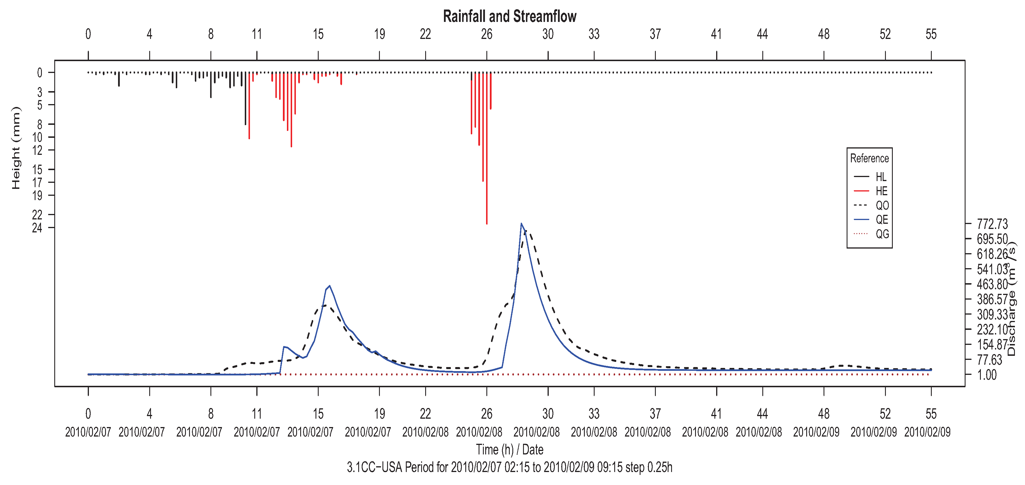
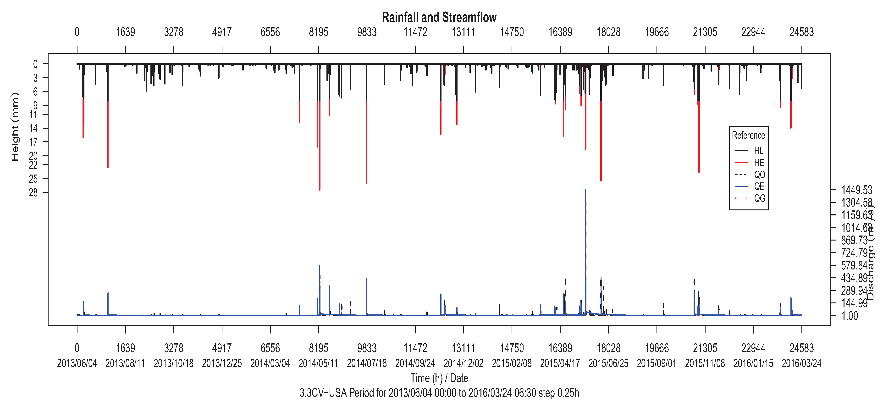
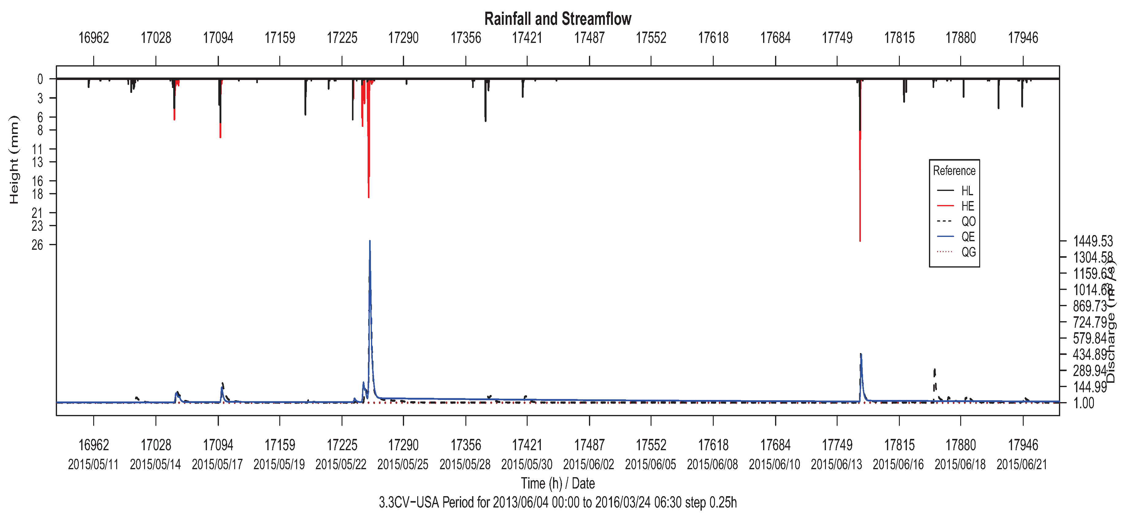
With respect to the San Antonio River, two hydrometric stations were considered, in Loop 410 and Goliad. The calibration and validation hietograms and hydrograms for the two stations are represented in Figure 12, Figure 13, Figure 14 and Figure 15, respectively.

It is worth noting that for San Antonio and Juquiá problem instances, similar hydrographs are obtained (see Figure 16 and Figure 17), which lead us to suggest that Qom is useful and accurate when applied to multiple and heterogeneous river basins and time periods.

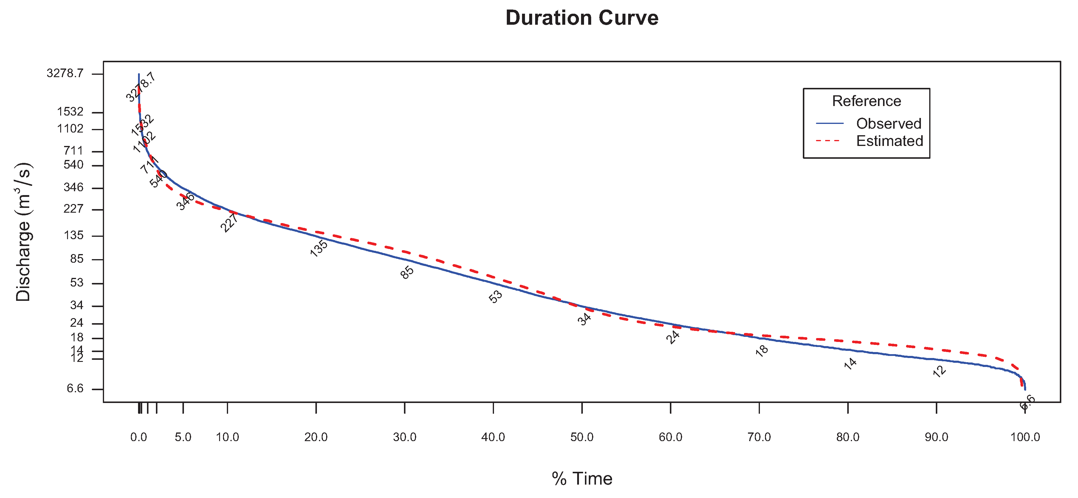
The hyetograph and hydrograph of the basin that belongs to Balapuca (Bermejo river) are shown in Figure 18. In this regard, an interesting comparison can be also extracted from the duration curve of the observed and estimated flows in Figure 19. It is another way to evaluate the behavior of the simulation model and the parameters, allowing to appreciate for which groups of flows better adjustments were obtained.

Resulting hydrographs in Figure 8 and Figure 19 reveal that observed streamflows are properly fitted by estimated ones in different problem instances and time periods.

6. Discussion

The main goal driving us in this work has been to provide a practical tool for hydrologic prediction based on the combination of two components—the Qom model and its automatic calibration using multi-objective optimization algorithms. The results reported in the previous section indicate that the Qom model is stable for a set of heterogeneous scenarios with different conditions and it does not produce large changes to small variations of the parameters. Therefore, it can be considered an adequate model for its use in the basin hydrological risk estimation, in basin climate change assessments, and in changes by use or soil practices.

A question that can arise is why have we proposed a new hydrologic model instead of using an existing one? The reason is related to the expertise of the paper authors, comprising hydraulic and computer science engineers. We are the creators of the jMetal software framework for multi-objective optimization metaheuristics. jMetal includes a large amount of algorithms representative of the state of the art but, as pointed out in Section 4.3, choosing which is the most promising one to solve a given optimization problem is not a easy task, in particular for experts in the application domain, which are usually not experts in the optimization techniques.

In this sense, a solution selection strategy is also suggested for guiding the expert in hydrology in the decision making process, which comprises the use of independent data series for calibration, as well as for validation, each of them involving different time periods of a given problem instance. This leads the proposal to select successful solutions that could be generated by calibration algorithms with low contribution in the Pareto reference front approximation, but with very stable results in terms of practical validation.

Our starting point was to use jMetal for the calibration of a hydrologic model; although this algorithmic library is implemented in the Java programming language, it hinders using existing models; for example, the Sacramental Soil Moisture Accounting (SAC-SMA) model is available in FORTRAN, Matlab, and R, but to the best of our knowledge there is no a Java version. Consequently, from our experiences in water resources we decided to define a new model—Qom—based on a reduced number of parameters to be adjusted, to implement it in Java, and integrating it into jMetal to use a multi-objective approach for automatic calibration, all aimed at providing a generic and accurate software tool that is freely available to the community.

Our objective in this paper has not been to compare Qom with existing models, nor to compare the automatic calibration scheme with existing strategies. These issues remain open and are included as lines of future work in the next section.

7. Conclusions

In this work, a novel hydrologic model called Qom is proposed to efficiently separate and quantify the volumes of losses and excesses of the rainwater falling in a hydrographic basin. In combination with it, an evolutionary multi-objective approach is used for parameter calibration focusing on indicators to qualify the adjustments between the observed and estimated hydrograms. A number of multi-objective algorithms in the scope of the jMetal framework are used to deal with the hydrologic model as a black-box optimization problem, with a vector of decision variables as inputs and objective function values as outputs.

The Qom model, featuring a reduced set of parameters, together with the possibility of using existing multi-objective optimizers without the need to tune each of them, just combining the solutions they produce, make this proposal of special interest for both academy and industry communities.

For testing purposes, six realistic hydrographic scenarios, comprising river basins located in Spain, USA, Brazil and Argentina, have been modeled and evaluated with different size conditions, climates, topographies, heterogeneous soils, and with series of very short time periods of 10, 15, 30 and 60 min and 24 h. The results indicate that the calibration of Qom of each problem allow to predict future storm flows as it is possible of accurately reproduce the phenomenon rain-runoff (cause-effect), thus fulfilling the goal of our work.

In general, the NSE and PBIAS obtained by Qom involved highly successful values of roughly 75% and 10% (respectively) in calibration, as well as in validation. This could be explained in terms of low errors of the predicted series with regards to observed ones, which can be classified as very satisfactory according to Reference [39]. Moreover, these results could even be improved if larger time periods of registration are considered, as we measure changing conditions from 10 min to 24 h, whereas references in the literature worked within monthly periods [39].

As lines of future work, an open issue to explore is the analysis of the Qom model when compared with other hydrological models, such as SWAT, VIC or SAC-SMA. Our proposal to combine different multi-objective metaheuristics can be time consuming, as a large number of independent runs of configurations of the algorithm/problem must be carried out. It would be more efficient to explore the use of automatic parameter tuning tools to determine if a single algorithm could be good enough. In this sense, a further step would be to self-generate an ad-hoc metaheuristic suited for the calibration of Qom. In both cases, the idea would always be to use automatic tools to avoid the expert to deal with algorithmic issues. The performance of the resulting method would be validated by comparing it with other parameter estimation techniques.