Article

SSNet: Learning Mid-Level Image Representation Using Salient Superpixel Network

1
School of Computer Science and Technology, Dalian University of Technology, No. 2 Linggong Road, Dalian 116024, China
2
Information Engineering College, Henan University of Science and Technology, No.263 Kaiyuan Avenue, Luoyang 471023, China
*
Author to whom correspondence should be addressed.
Appl. Sci. 2020, 10(1), 140; https://doi.org/10.3390/app10010140
Submission received: 7 November 2019 / Revised: 13 December 2019 / Accepted: 20 December 2019 / Published: 23 December 2019
(This article belongs to the Section Computing and Artificial Intelligence)

Abstract

:
In the standard bag-of-visual-words (BoVW) model, the burstiness problem of features and the ignorance of high-order information often weakens the discriminative power of image representation. To tackle them, we present a novel framework, named the Salient Superpixel Network, to learn the mid-level image representation. For reducing the impact of burstiness occurred in the background region, we use the salient regions instead of the whole image to extract local features, and a fast saliency detection algorithm based on the Gestalt grouping principle is proposed to generate image saliency maps. In order to introduce the high-order information, we propose a weighted second-order pooling (WSOP) method, which is capable of exploiting the high-order information and further alleviating the impact of burstiness in the foreground region. Then, we conduct experiments on six image classification benchmark datasets, and the results demonstrate the effectiveness of the proposed framework with either the handcrafted or the off-the-shelf CNN features.

1. Introduction

Image classification aims to categorize a set of unlabeled images into several predefined classes according to their visual content. Learning the mid-level image representation is important to image classification task. To exploit the mid-level information, bag-of-visual-words (BoVW) [1] and convolutional neural networks (CNN) models [2] are two typical kinds of methods. For BoVW methods, sparse coding with spatial pyramid matching (ScSPM) [3], locality-constrained linear coding (LLC) [4], and vector of locally aggregated descriptor (VLAD) [5] usually encode and aggregate handcrafted features such as scale invariant feature transform (SIFT) features [6] and Dense SIFT features [7] to form the high-dimensional mid-level representation. Recently, off-the-shelf CNN local features are also applied in image classification tasks. In [8], the authors perform the VLAD pooling of the CNN local features extracted from the full-connected layer to form the mid-level image representation. Liu et al. in [9] designed the image representation with the CNN local features extracted from the convolutional layers.
Although the BoVW representation models based on the handcrafted or the off-the-shelf CNN features have achieved appealing results, they may suffer from the following two drawbacks:
(1)
Susceptible to the interference of the burstiness. Burstiness is a phenomenon in which frequently occurring features, often carrying little information about the object, are more influential in the image representation than rarely occurring ones in the natural image [10,11]. As demonstrated in Figure 1, a large number of similar and less informative features occur in the background and will weaken the discriminative power of the representation. To solve it, Russakovsky et al. [12] and Angelova et al. [13] introduce location information to separate the foreground and background features and form the image representation. These methods have enhanced the discriminative ability of the representation; however, training an object detector is time-consuming. Ji et al. [14] and Sharma et al. [15] build the image representation by using saliency maps to weight the corresponding visual features. Nevertheless, they ignore the difference between features in the detected salient regions. In addition, normalization or pooling operations [16,17] are proposed to deal with the burstiness issue. However, the spatial relationship between features are usually ignored, which is important for alleviating the burstiness phenomenon of the features.
(2)
Ignoring the high-order information. The traditional BoVW method and its variants usually use the first-order statistics of features to form the image representation. However, the high-order information can provide more accurate representation for images [18,19]. The lack of the high-order information will limit the performance. To address it, Huang et al. [20] and Han et al. [21] utilize high-order information for building feature descriptors. However, simply introducing the high-order information into the design of the feature descriptor contributes little to improve the performance of image classification tasks. Sanchez et al. [22] and Li et al. [23] introduce the second-order information in the encoding procedure. However, they only use the second-order information of each visual word itself and ignore the relations between the visual words. To solve it, the research [18,19,24] introduces the high-order information between the visual words with the use of the pooling strategy.
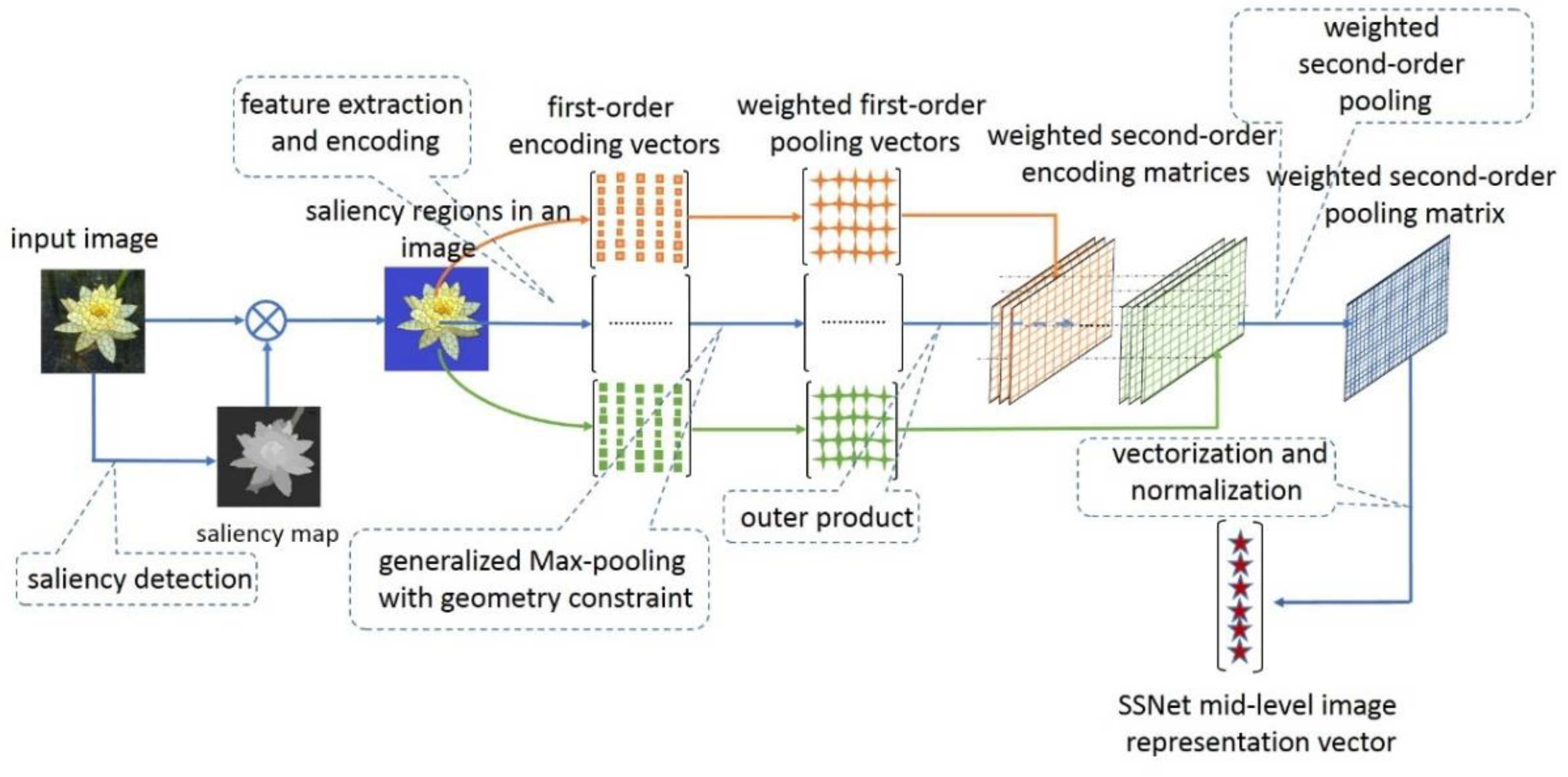
To address the two above-mentioned problems, we propose a novel representation framework called Salient Superpixel Network (SSNet) in this paper. Inspired by the Gestalt grouping principle, in which the human visual system tends to perceive objects that are similar, close, or connected without abrupt directional changes as a perceptual whole, we introduce a visual saliency detection module to highlight the salient regions in the image and reduce the interference of the burstiness inside the background region. Then, a weighted second-order pooling scheme is proposed to balance the influence of the features and incorporate the higher-order information for generating more discriminative representation. Figure 2 demonstrates the pipeline of the proposed framework.
The main contributions of the proposed framework can be summarized as the following ones:
(1)
A fast saliency detection model based on the Gestalt grouping principle is proposed to highlight the salient regions in the image. With the use of the saliency strategy, only the features inside the salient regions are extracted to represent the image. As a result, the interference of the burstiness inside the non-salient regions can be weakened.
(2)
Based on the similarity and spatial relationship between the features, we propose a novel weighting scheme to balance the influence between the frequently occurring and rarely occurring features, and in the meantime reduce the side effects of the burstiness.
(3)
To introduce the high-order information and further downplay the influence of the burstiness, we conduct the power normalization based on the proposed weighted second-order pooling operation. Consequently, more discriminative representation is achieved.
The rest of the paper is organized as follows. First, the related work is discussed in Section 2. In Section 3, we mainly describe the proposed mid-level image representation framework. In this part, the proposed saliency detection method and weighted second-order pooling scheme will be introduced in detail. Finally, we conduct extensive experiments on the benchmark datasets. The experimental results and corresponding analysis are presented in Section 4. The conclusion is described in Section 5.

2. Related Work

In this section, we first introduce the recent research on mid-level image representation and the commonly used methods for extracting the off-the-shelf CNN local features. Then, the studies on the burstiness problem are reviewed. Finally, the research on image representation with high-order information are discussed.

2.1. Research on Mid-Level Image Representation

Learning a robust and discriminative image representation is a critical issue for image classification. Over the years, researchers have proposed a wide variety of representation methods. Typically, these methods can be categorized into three levels: high level, mid level, and low level. The high-level representation usually offers discriminative power by conveying semantic or prior knowledge about objects. However, the data-driven based high-level information requires a large number of human-labeled tags. Low-level methods often use the basic features obtained from some various hand-crafted descriptors, such as SIFT [6] and histogram of oriented gradients (HOG) [25], to represent the images. Despite many more informative descriptors being put forward, the performance of low-level representation methods still remain limited. Recently, several approaches have been proposed to transform low-level features into the mid-level representation. It is more informative and discriminative than the low-level one and is able to bridge the semantic gap between the low-level and high-level representation.
At present, bag-of-visual-words (BoVW) and convolutional neural networks (CNN) models are often applied to learn the mid-level image representation. Over the years, researchers have proposed a wide variety of image representation methods based on the bag-of-visual-words model. This model mainly consists of the following four stages. (1) Feature extraction. Traditionally, local features such as SIFT [6] and Dense SIFT [7] have been widely used for representing images. (2) Building the codebook. Usually, K-means or the Gaussian Mixture Model (GMM) clustering algorithm is used to build the codebook. (3) Feature encoding. In this stage, extracted local features are encoded by the learned codebook. There are some classic encoding methods, such as locality-constrained soft assignment (LCSA) [26], soft assignment (SA) [27], fisher vector (FV) [22], and vector of locally aggregated descriptor (VLAD) [5]. FV has achieved state-of-the-art results in several recognition tasks before the emergence of the Deep Learning. (4) Pooling operation. The pooling operation aggregates all the encoded features to form the final representation vectors for the images, and average pooling and max pooling are often used.
In addition, the research [7,28] obtains the mid-level representation by pooling more discriminative information than the standard BoVW model does. Ronan Sicre et al. [29] propose a novel descriptor that encapsulates the mid-level information based on superpixel structure. Yuan et al. [30] generate visual phrases via combining the visual words depending on the co-occurrence of them. Mayank Juneja et al. [30] propose a novel method to learn distinctive parts of objects or scenes automatically in a supervised way. With the learned parts, a discriminative mid-level representation is generated.
Recently, convolutional neural networks (CNNs) have been successfully applied to various computer vision tasks such as image classification [2,31,32] and object detection [33,34]. Such great success spurs a flurry of research work on further improving CNN architecture [32,35], as well as on using CNN features as a universal representation for recognition [36,37,38]. Additionally, several works extract the local intermediate activations from a pretrained CNN model and aggregate them to generate a generic mid-level representation, i.e., the representation based on an off-the-shelf CNN model. The CNN-based representations achieve state-of-the-art performance in wide visual recognition tasks [8,39,40,41,42].
In this paper, we mainly discuss the mid-level representation based on BoVW with the handcrafted and off-the-shelf CNN local features.

2.2. Methods of Extracting the Off-the-Shelf CNN Feature

In general, there exist two main ways of extracting features from pretrained CNN models. The first one takes the activations from the last fully connected layer as features [8,43,44], and the second extracts features from the convolutional layer [9,41].
For the methods of the first kind, when a whole image is input into a pretrained CNN model, the activation extracted from the fully connected layer is often employed as a universal image representation. In addition, when an image patch is input, the activation can be used as a local feature of the patch itself. In this situation, we can achieve an image representation via pooling lots of CNN local features extracted from the image.
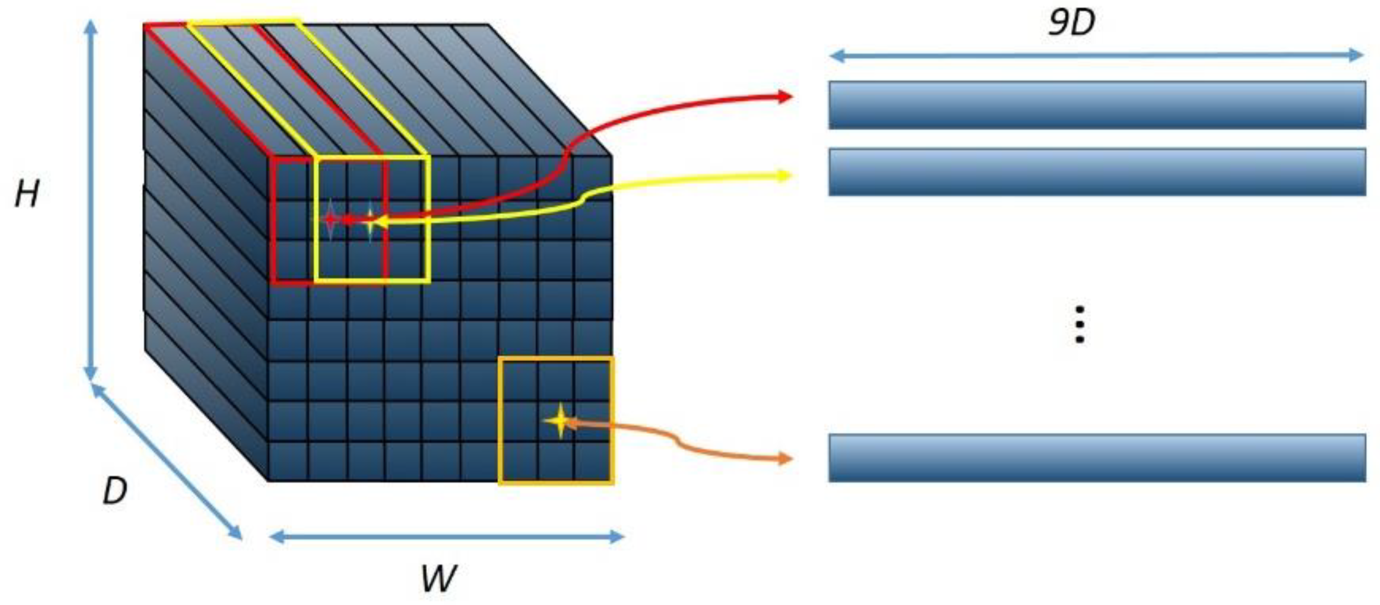
Recently, the activations from the convolutional layer are often exploited to represent an image [9,41], which contain more rich spatial information than the fully connected layer ones. The activations extracted from the convolutional layer form a H×W×D tensor, where H and W denote the height and width of each feature map, and D denotes the number of the feature maps, as shown in Figure 3. Further, the tensor can be viewed as a set of D-dimensional vectors extracted at H×W spatial locations, and each D-dimensional element can be considered as a feature descriptor. The studies [45,46] have pointed out that the discriminative power of this kind is weaker than the activations of the fully connected layer. In order to deal with this issue, Liu et al. [9] propose a novel feature extraction method, which takes a set of sub-arrays of convolutional layer activations as the local features. As demonstrated in Figure 3, they first extract nine D-dimensional feature vectors from the red box region and concatenate them into a 9D-dimensional feature; then, they shift one unit along the horizontal direction to extract features from the yellow box region. With the same operation, scanning all the feature maps, a large number of 9D-dimensional enhanced local features are obtained. In our framework, we adopt the same method as in [9] to extract CNN local features.

2.3. Research Work about Burstiness Issue

In [10], Jegou et al. point out the burstiness phenomenon and analyze its effect on object recognition tasks. In the context of image classification, burstiness weakens the discriminative ability of an image representation.
In order to deal with the burstiness interference originating from the background area of an image, the studies [12,13,47] use a detector to locate the object first and then pool the foreground and background features separately to form the mid-level representation. In [12], Russakovsky et al. propose a framework that directly optimizes the classification objective with treating object detection as an intermediate step. For the fine-grained object classification task, Anelia Angelova et al. [13] introduce the object detection and segmentation algorithm to localize and normalize the object. They segment the possible object of interest before trying to recognize it. Although this method alleviates the impact of the burstiness to some extent, the obtainment of pretrained detectors is a time-consuming procedure. In addition, some methods [14,15,48,49] are proposed to weight different regions by saliency values. In [15], Sharma et al. extend the notion of discriminative visual saliency by including discriminative spatial information and obtain a more discriminative image representation for visual classification. Ji et al. [14] propose a new feature generation approach by encoding the salient object region information to the histogram-based features for image classification. However, in these methods, the difference between features in the detected salient regions is ignored.
For the burstiness phenomenon happening in the foreground region, researchers [11,17,50] try to solve it by the proposed normalization or pooling operation. In [50], Perronnin et al. use the power normalization technology to adjust the feature distribution. In [11,17], the authors adopt separately the Max-pooling and Generalized Max Pooling operation to reduce the impact of the burstiness.
In the SSNet framework, a novel saliency detection method is proposed first to alleviate the side effect of the burstiness inside the non-salient regions of an image. Then, we further put forward a novel weighting scheme to balance the influence between the frequently occurring and rarely occurring features, and reduce the side effect of the burstiness in the object regions.

2.4. Image Representation with Second-Order Information

Second-order statistical information has played an important role in advancing the discriminative power of an image representation. In recent years, the numbers of novel descriptors [20,51] are designed to capture the second-order information. Tuzel et al. [51] present a covariance descriptor that describes a patch by utilizing the covariance statistics of its inner pixels. In [20], Huang et al. provide a way to embed the second-order gradients of pixels into a descriptor. Additionally, many second-order feature encoding methods are also put forward successively. For example, fisher vector (FV) [22] makes use of the first-order and second-order information of the hand-crafted features. The locality-constrained affine subspace coding (LASC) [23] uses the fisher information matrix for improving the representing power. Recently, the research [19,24] introduced the second-order information at the pooling stage.
The method proposed in [19] shares similar intentions with us. The main difference is that our method combines the second-order pooling operation with the weighting scheme, which not only introduces the high-order information but also alleviates the side effect of the burstiness.

3. The Proposed Method for Image Representation

In this section, the SSNet image representation framework will be demonstrated. First, the proposed saliency detection approach is depicted, and then the weighted second-order pooling method is introduced in detail. Finally, the overall description for the SSNet image representation is presented.

3.1. Saliency Region Detection

In order to alleviate the impact of burstiness in the background of an image, we use salient regions instead of the whole image for extracting features. As described in our previous work [52], a path-based background saliency model is introduced to uniformly detect the salient region in the image. Specifically, the method first applies the path analysis based on Gestalt grouping principle to represent the topology structure between image pixels, and then integrates the topological connectedness and appearance contrast for modeling the saliency. To enhance the efficiency, this paper proposes a fast implement of the path-based background saliency model based on the two-stage traversal on the minimum spanning tree, which is more efficient than the original one [52]. Note that in the following subsection, only the enhanced path analysis method and the saliency map generation procedure are depicted. For more background knowledge, please refer to the work [52].

3.1.1. Measuring the Gestalt Grouping Connectedness

(1) Minimum bottleneck distance transform
Inspired by the fact that the human visual system tends to perceive objects that are similar, close, or connected without abrupt directional changes as a perceptual, we have proposed the smoothest path to represent the relation between image pixels based on the similarity, local proximity, and global continuity of the Gestalt grouping principle, that is
P s ( A , B ) = m i n p P A , B { m a x p [ h ] , p [ h + 1 ] p { w p [ h ] p [ h + 1 ] } }
where P A , B denotes the set of all paths linking node A and node B on the k-nearest neighbor graph, p [ h ]   is the hth node on the path p from node A to node B, and the largest edge weight on each path p is defined as the bottleneck to limit the performance of that path. The smoothest path P s between A and B signifies the path that minimizes the largest edge weight of all the paths P A , B . In addition, it has been proven that the path between two nodes in a minimum spanning tree (MST) of a graph is one of the smoothest paths for that pair of nodes.
From the perspective of distance transform, we call the metric defined in Equation (1) the minimum bottleneck distance to emphasize the features represented by the smoothest path. Given a distance metric g ( π ) , the distance transform of a node v is defined as
D ( v ) = m i n π Π S , v g ( π ) .
Π S , v is the set of all paths between v and a seed in   S ,   π = { π ( 1 ) , π ( 2 ) , , π ( k ) } is a path belonging to Π S , v , and g ( π ) denotes each kind of distance metric following the properties of symmetry and non-negativity. In Equation (1), g ( π ) becomes
g ( π ) = m a x i = 1 k 1 | I ( π ( i + 1 ) ) I ( π ( i ) ) | .
Furthermore, the calculation of the minimum bottleneck distance between a pair of nodes can be achieved by finding the largest edge weight of the path on the MST.
(2) Two-stage traversal on the MST
In [53], Tu et al. applies the MST instead of the whole graph to approximately calculate the geodesic distance and minimum barrier distance in linear time. Similar to that, we propose a fast implement of the minimum bottleneck distance with the use of the bottom–up traversal and top–down traversal.
Given a set of seed nodes S , for each node s S , its corresponding distance value is set to 0. For other nodes, their distance values are set to , as shown in Figure 4a. For the bottom–up pass, we start from the leaf nodes and update the distance values of their parent nodes with
D ( v p ) = m i n { D ( v p ) , g ( π v q v p ) }
where v p is the parent node of the visited v q , π v q is the current optimal path that connects v q and its nearest seed node, and π v q v p means that the path π v q walks one step further to arrive at node v p . This process does not end until it reaches the root node. Figure 4b demonstrates an example of the bottom–up pass.
For the top–down pass, we start from the root node. Figure 4c demonstrates an example of the top–down pass. For each node v q , we update its distance value from the parent node. That is,
D ( v q ) = m i n { D ( v q ) , g ( π v p v q ) } .
As shown in Figure 4, we should track the maximum value of each node. When we visit a newly added node, two comparison operations are required for either the bottom–up or top–down traversal. Specifically, one comparison is for recording the largest edge weight of the path, and the other comparison is used to determine whether the current distance is smaller than the new one. If it is smaller, the corresponding distance value remains unchanged; otherwise, we update the value with the current one. After the two-stage traversal, we can achieve the minimum bottleneck distance transform D for each pair of nodes on the graph.
(3) Gestalt grouping-based connectedness
Compared with the object regions, most of the background ones are easily connected to image boundaries. Based on the observation, the saliency of an image pixel is defined as the topology connectedness to the image background. Given the background seed pixels B t and the minimum bottleneck distance transform D , the connectedness of each pixel i in the image can be calculated by
  C t ( i ) = m i n b ϵ B t ( D ( i , b ) ) .
Different from previous methods in which the pixels on the image boundary are simply regarded as background seeds, we introduce the iterative background growth algorithm in the paper. In other words, we first initiate the set B with the boundary pixels B d , and then update the B t when the saliency values of the pixels belonging to B d exceed the threshold, that is
B 0 ( i ) = { i | i ϵ B d }
  B t ( i ) = { i | i ϵ B t 1 ( i ) , C t 1 ( i ) < θ t 1 }
where θ t 1 is the mean value of C t ( i ) for all pixels in set B t 1 ( i ) . The iterative process defined in Equations (6) and (8) will terminate when B t is unchangeable or i C t ( i ) C t 1 < ε .
If there exists a scattered background or objects heavily touch the image border, the connectedness may falsely inhibit the object region. To tackle it, the appearance contrast between objects and background are used for highlighting the high-contrast objects.
Let c ϵ { 1 ,   2 ,   3 ,   4 } denote the left, right, top, and bottom regions of the image border B d . For each boundary region c , x ¯ c = [ x ¯ L ,   x ¯ a ,   x ¯ b ] is the mean color for all the pixels in the CIE-Lab color space, and Q c = [ q i j ] 3 × 3 is the corresponding color covariance matrix. The appearance contrast between each pixel and the border region c is defined as
a c i = ( x i x ¯ c ) Q c 1 ( x i x ¯ c ) T ,   c ϵ { 1 ,   2 ,   3 ,   4 } .
Equation (9) describes the Mahalanobis distance between pixel i and the mean color. Then, the generated a c i is normalized with the maximal value.
  a c i a c i m a x i a c i
Therefore, the appearance contrast is calculated by accumulating a c i from the four boundaries.
A ( i ) = c = 1 4 n c a c i 4 n c
where n c is the number of image pixels belonging to the boundary region c .

3.1.2. Saliency Map Generation

The connectedness map C and the appearance map A are added in the pixelwise way to form the final saliency map M i.e.,
M = C + A .
The achieved saliency map incorporates not only the topology structure but also the feature difference between image pixels to detect the salient regions in the image.

3.2. Image Representation with the Weighted Second-Order Pooling

3.2.1. The Proposed Feature Weighting Method

In this section, we will present the proposed feature weighting method, which can be considered as an improvement of the generalized max pooling approach [11]. Next, we first introduce the generalized max pooling approach.

Generalized Max-Pooling Method

In order to alleviate the side effect of the burstiness, Murray et al. [11] propose the generalized max-pooling (GMP) method, which equalizes the contribution of the frequently occurring and rarely occurring descriptors to the image representation.
Let X = { x 1 , , x N } be a set of N feature descriptors extracted from an image and φ n = φ ( x n ) denote the D-dimensional encoding result of the n th descriptor. Assuming that φ g m p denotes the GMP representation, the GMP method enforces the dot-product between each feature encoding result φ n and GMP representation φ g m p to be a constant c :
φ n T φ g m p = c ,   n = 1 , , N .
Here, the constant c can be set as an arbitrary value, as the final representation φ g m p typically need to be L2 normalized. Therefore, the authors assign   c = 1 . Equation (13) ensures that each feature descriptor makes the same contribution to the final pooled representation.
Further, let Φ denote a D × N matrix that contains N D-dimensional feature encoding results, i.e., Φ = [ φ 1 , , φ N ] . Then, Equation (13) can be represented in matrix form:
Φ T φ g m p = Ι N
where Ι N denotes a N-dimensional vector of all ones. This is a linear system of N equations with D unknowns. In general, this system might not have a solution. Thus, Equation (14) can be transformed into a least-squares regression problem with the additional constraint that φ g m p has a minimal norm in the case of an infinite number of solutions:
  φ g m p = a r g m i n | | Φ T φ Ι N | | 2 φ   .
This problem has a simple closed-form solution:
  φ g m p = ( Φ T ) + Ι N = ( Φ Φ T ) + Φ Ι N .
Note that Φ Ι N = n = 1 N φ ( x n ) = φ s u m is the sum-pooled representation. Hence, the proposed GMP can be considered as the result of projecting φ s u m   onto the ( Φ Φ T ) + .
Since the ( Φ Φ T ) + is not a continuous operation, the authors further introduce φ   λ g m p , the regularized GMP, and try to obtain a stable solution:
φ   λ g m p = a r g m i n { | | Φ T φ Ι N | | 2 + λ | | φ 2 | | } φ   .
This is a ridge regression problem whose solution is
φ   λ g m p = ( Φ Φ T + λ E ) 1 Φ Ι N
where λ   is a regularization parameter and E is an identity matrix.
If Equation (18) is rewritten as the weighted pooling form
  φ   λ g m p = Φ α λ
where α λ is the vector of weights, and let   φ = Φ α in Equation (17), then the weight α λ   can be obtained by:
α λ = a r g m i n { | | Φ T Φ α Ι N | | 2 + λ | | Φ α 2 | | } a   .
Let K = Φ T Φ , which represents a N × N matrix of descriptor-to-descriptor similarities; then, Equation (20) can be represented as:
α λ = arg   m i n { | | K α Ι N | | 2 + λ a T K a } a   .
Finally, a simple weight solution is obtained:
α λ = ( K + λ E ) 1 Ι N .
For more details about GMP, please refer to the work [16].

Weighting Scheme with Geometry Constraint

Based on the analysis above, we know that the GMP can be regarded as a weighting method, which alleviates the side effect of the burstiness. However, this method only makes use of the similarity of features but ignores the spatial relationship between them. Thus, inspired by Equation (21), we define a novel weighting function as follows, which incorporates the spatial constraint,
w = a r g m i n { | | K w Ι N | | 2 + λ 1 w T K w + λ 2 w T S w } w  
where S is a N × N symmetric metric matrix. The element s i j represents the distance between the feature descriptors and is defined as:
  s i j = e x p ( | x i x j | w i d t h + | y i y j | h e i g h t 2 σ 2 )
where ( x i , y i ) and ( x j , y j ) denote the position information of the feature i and j , respectively, and σ is the smoothing coefficient. The setting of variable w i d t h and h e i g h t will be specified in Section 3.3. Finally, we get a simple solution:
w = ( K 2 + λ 1 K + λ 2 S ) 1 ( K Ι N )
and the w can be used to weight the corresponding features.

3.2.2. Weighted Second-Order Pooling

In order to introduce the second-order information, two novel feature pooling methods will be presented, which are based on a collection of independent superpixels.
Given an image, we segment it into a set of M superpixel regions R = ( R 1 , R M ) by the simple linear iterative cluster (SLIC) method [54]. Assuming that there exist N i feature descriptors in the region R i , we encode them with the method φ ( · ) and obtain the corresponding coding matrix Φ i = [ φ 1 , , φ N i ] . According to Equation (25), the related weighting vector w i can be determined.
Based on Equation (19), the weighted first-order pooling ν i for the region R i is defined as:
ν i = Φ i w i
which can be considered as a representation vector for the region R i .
For an image, we define the weighted second-order average pooling (WSOAP) as:
W S O A P = 1 M i = 1 M ν i · ν i T .
Here, the result of ν i · ν i T is a matrix, which contains the second-order statistical information about the features inside the region R i . The WSOAP captures the second-order information included in the M regions of an image.
Correspondingly, we define the weighted second-order max pooling (WSOMP) as
W S O M P =   m a x i = 1 : M { ν i · ν i T }
where the max operation acts on the corresponding elements with the same position of the matrices resulting from the outer products of the weighted first-order pooling vectors.

3.2.3. Vectorization and Normalization

We are interested in using linear classifiers to implement the classification task, which offers linear training time. Linear classifiers, such as SVM, often work well in Euclidean space, which optimize the geometric margin between positive and negative examples in vector form. Meanwhile, the WSOAP and WSOMP are both symmetric matrix ( S n ) , so they need to be vectorized.
Specially, the WSOAP is a symmetric and positive semi-definite matrix ( S n + ) . The space of S n + forms a Riemannian manifold, which is a differentiable manifold endowed with a Riemannian metric [55]. So, for the WSOAP, based on the properties of the Riemannian manifold [56], we map it to the Euclidean tangent space by using the Log-Euclidean metrics, i.e.,
W S O A P l o g m = l o g m ( W S O A P ) .
Here, the result W S O A P l o g m is still a symmetric matrix.
To the WSOMP, the power normalization mapping [50] is adopted, which is able to further reduce the influence of the burstiness. For each entry W S O M P ( i , j ) of WSOMP, we have
W S O M P ( i , j ) P N M = s i g n ( W S O M P ( i , j ) ) | W S O M P ( i , j ) | α
where α is a hyper parameter controlling the magnitude, which is usually with the range of ( 0 , 1 ] .
As either W S O A P l o g m or W S O M P P N M is symmetric, the upper triangle elements are unpacked and concatenated into a vector to form the final representation, i.e.,
W S O A P f i n a l = V e c t ( U ( W S O A P l o g m ) )
W S O M P f i n a l = V e c t ( U ( W S O M P P N M ) )
where U ( · ) indicates the operation of obtaining the upper triangle elements and V e c t ( · ) denotes the vectorizing operation.

3.3. The Mid-Level Image Representation Based on SSNet

In the SSNet representation framework, in order to reduce the side effect of the burstiness in the background of an image, the saliency detection method proposed in Section 3.1 is applied, but here, superpixels not pixels are used to generate the saliency map. After that, only the patches with the top-S large salient value are used to represent the image. Here, we set
S = [ N u m S u p p i x e l i m g R a t i o s a l ]
where N u m S u p p i x e l i m g is the number of the superpixels included in an image, and R a t i o s a l is a predefined constant that represents the ratio between the number of the chosen saliency superpixels and the total number of the superpixels in an image.
At the same time, in order to introduce higher-order feature information, the weighted second-order pooling is proposed. For each saliency superpixel R i ,   i = 1 , 2 , S , we extract M i features x i j ,   j = 1 , 2 , M i , and encode them by the encoding method φ ( · ) . Assuming the matrix Φ i = [ φ i 1 , , φ i M i ] includes encoding outcomes of the features inside in the superpixel R i   , we can obtain the weight vector w i for the Φ i based on Equation (23). Further, using Equation (26), the first-order pooling results for patch R i ,   i = 1 , 2 , S can be decided. After that, we can get the weighted second-order pooling result with the proposed methods in Section 4.2, and achieve the final representation using the approaches in Section 4.3. Figure 5 illustrates the pipeline of the SSNet image representation.
In this paper, we try to adopt two different features respectively to build the SSNet image representation. (1) Dense SIFT. We extract Dense SIFTs within each superpixel region and encode them by the BoVW way. And the variable w i d t h and h e i g h t in Equation (24) are set as the width and height of an input image respectively. (2) Off-the-shelf CNN local features. For each superpixel, we input the region of its circumscribed rectangle into a pretrained CNN model and extract the CNN local features by the way in [9] as mentioned in Section 2.2, and the variable w i d t h and h e i g h t in Equation (24) are set as the width and height of the feature map, respectively.
The proposed image representation method based on the SSNet is summarized in Algorithm 1.
Algorithm 1: Generating the SSNet Mid-Level Image Representation
Input: a. Input image I
    b. R a t i o s a l , the ratio between the number of the chosen saliency superpixels and the
     total number of the superpixels in an image
    c. D f , the reduced dimension of the feature f i
    d. D c , the reduced dimension of the encoding vector
 Output: The final mid-level representation F i n a l R e p for the input image
    1. Computing the saliency map of the image I ;
    2. Computing the S , the number of salient regions used to represent an image, using Equation (33);
    3. Choosing the salient regions S R = { s r 1 , s r 2 , s r S } with the top- S saliency value;
    4. for i = 1:S
      4.1 Extracting N i Dense SIFTs/CNN local features from s r i and reducing their
         dimensionality to D f ;
      4.2 Encoding the features, reducing the dimensionality of the codes to D c , and
         achieving the coding matrix Φ i = [ φ 1 , , φ N i ] ;
      4.3 Computing the weight w i for the codes using Equation (25);
      4.4 Computing the first-order pooling vector v i for the salient region s r i
         using Equation (26);
     end
    5 Computing the second-order pooling W S O A P /   W S O M P for the image using Equation
      (27)/Equation (28);
    6 Mapping or Normalizing the W S O A P /   W S O M P using Equation (29)/Equation (30);
    7 Obtaining the final representation F i n a l R e p for image I by vectorizing operation
       using Equation (31)/Equation (32).

4. Experiments and Results

In this section, we carry out a series of experiments to investigate the effectiveness of the SSNet framework. First, the experiment setting and the datasets used are introduced. Then, integrating with four BoVW baseline methods, including ScSPM [3], LLC [4], FV [22], and VLAD [5], we assess the benefit of the saliency detection scheme and the weighted second-order pooling method. Finally, we evaluate the overall performance of the SSNet mid-level representation with the handcrafted and off-the-shelf CNN local features, respectively.

4.1. Experimental Setting

In the experiment, we use the Dense SIFT local features and the off-the-shelf CNN local features respectively to evaluate the proposed methods. All the algorithms are implemented by the VLFeat [57] and Matconvnet toolbox [58]. The setting for the CNN local features follows the description in Section 2.2. For Dense SIFT features, they are extracted densely from local patches with a stride of four pixels on each image, and PCA is applied to reduce the dimensionality to 64. In the BoVW representation, a codebook containing K visual words is built via K-means clustering, and the value K varies across different datasets. In addition, the σ in Equation (24) is set to 1. With the same settings as [16], the λ 1 , λ 2 in Equation (25) is chosen by cross-validation from the set { 10 1 , 10 2 , 10 3 , 10 4 , 10 5 } , and the α in Equation (30) is set to 0.5. The setting for other parameters will be discussed in the following subsection. For each dataset, the experiments are repeated five times, and the average accuracy is reported.

4.2. Benchmark Datasets

15-Scene This dataset consists of 4485 scene images that belong to 15 different categories. Each category contains about 200–400 images, with an average size of 300 × 250. In the experiments, we test our method by randomly selecting 100 training images per class and using all the rest for testing.
Pascal VOC 2007 This dataset is a challenging benchmark, which consists of 9963 images from 20 classes. There are large in-class divergence, including variation on scale, illumination, and deformation, as well as severe object occlusions. Here, we choose this dataset as a sample to demonstrate the parameter setting for the SSNet.
Caltech 101 This dataset is one of the most commonly used datasets for image classification. It contains 9146 images from 101 object categories and one background category. The number of images per category varies from 40 to 800. In our experiments, we randomly select 30 training images and at most 50 testing image and ignore the background class.
Caltech 256 This dataset consists of 30,607 images divided in 256 categories, containing at least 80 images each. Compared to Caltech 101, it presents a much higher variability in object size, location, and pose. In the experiments, we randomly select 45 training images per class and all the rest for testing without evaluating the background class.
PFID61 The dataset contains 1098 fast-food images belonging to 61 different food categories, with masked foreground [59]. Each food category includes three different instances. For each instance, six images are collected from six viewpoints. In the experiments, 12 images from two instances are used for training and six images are used from the third instance for testing.
Food101 The dataset contains 101,000 images divided in 101 food categories [60]. Each category contains 1000 images, and all the images are rescaled to have a maximum side length of 512 pixels. In the experiments, 750 images are used for training and 250 images are used for testing.

4.3. Effectiveness Evaluation of the Proposed Saliency Detection Scheme for Image Classification

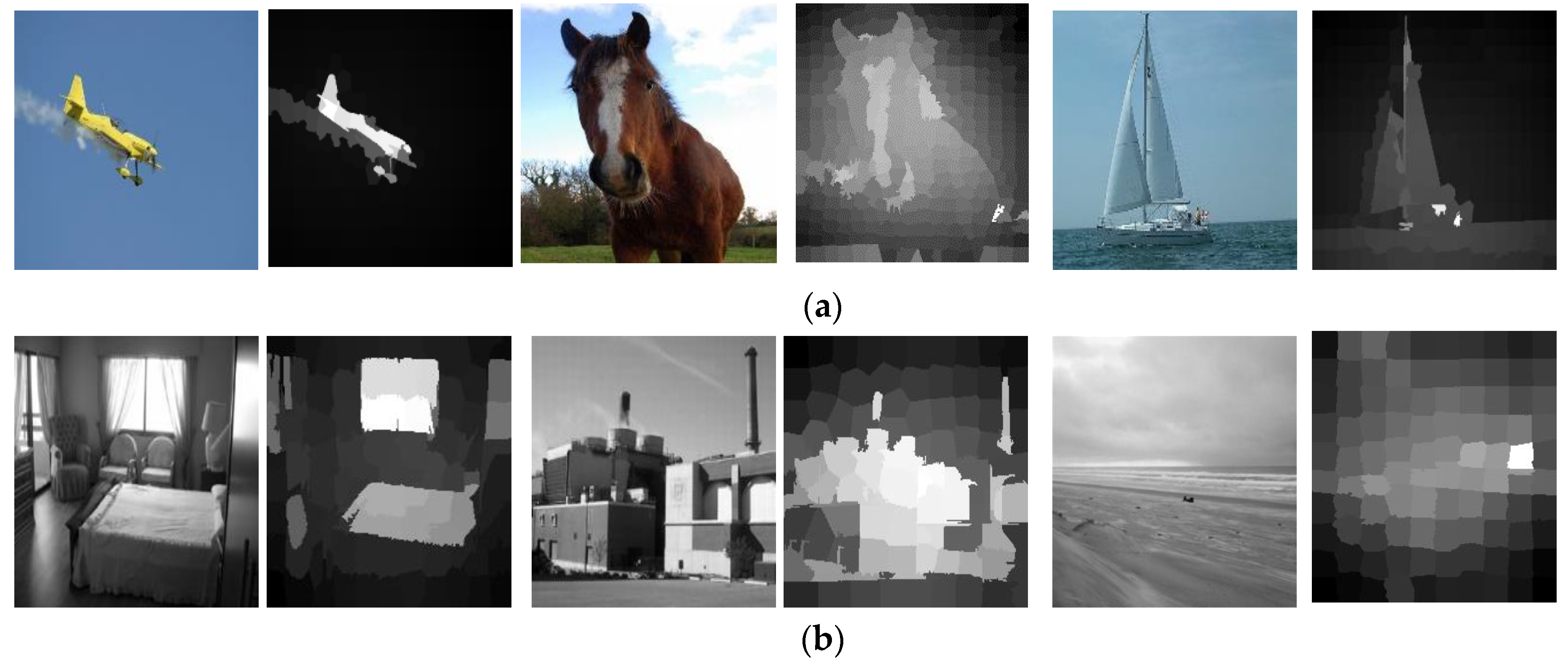
Generally speaking, for an image, the objects often exist in the saliency region and the background corresponds to the non-saliency region. Thus, we propose a novel representation method that roughly divides an image into object and background region first by saliency detection technology and then only choses the saliency regions to represent an image. By this way, the side effect of burstiness and noise information in the background can be alleviated. To this end, a fast saliency detection algorithm based on the Gestalt grouping principle is proposed. Figure 6 presents some saliency maps produced by the proposed saliency detection algorithm on the sample images taken from the Pascal VOC 2007 and 15-Scene datasets.
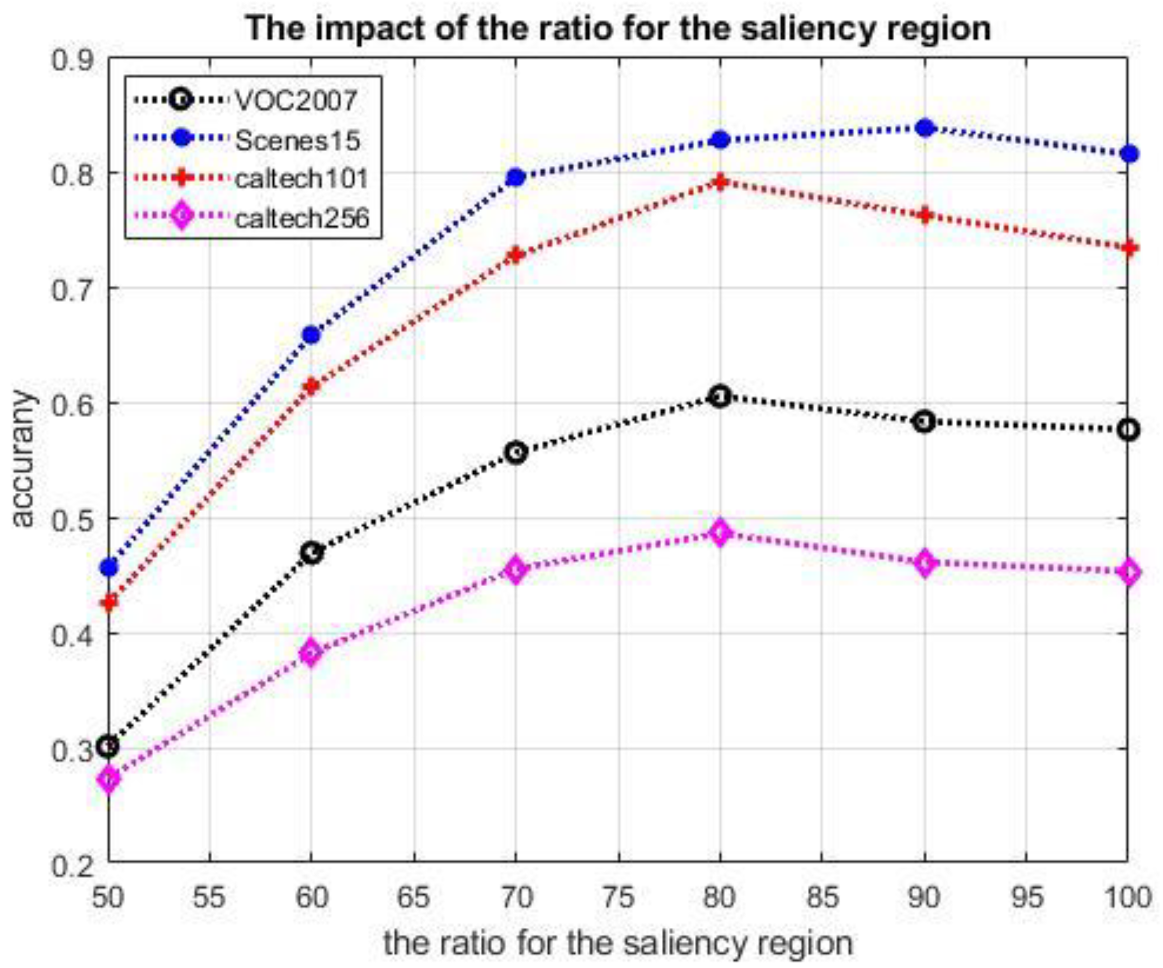
As mentioned in Section 3.3, in the proposed method, only the patches with a top- S large salient value are used to describe an image. The value of the S is a key parameter, which affects the performance of the representation. In Equation (33), we assume that the N u m S u p p i x e l i m g is a constant, and the value of S is in proportion to R a t i o s a l . So, the performance of our method can be considered as a function of R a t i o s a l . Figure 7 shows the curve of the mAP of our approach on the benchmark datasets with the different R a t i o s a l . Here, we take the LLC encoding method [4] as an example and integrate it with the saliency detection scheme to present the images. In the experiments, all the settings for LLC are in accordance with the work [4] except that the SPM technology can only be adopted under the condition of R a t i o s a l = 100 % (note that R a t i o s a l = 100 % denotes the original LLC method, i.e., without introducing the saliency detection scheme). As shown in Figure 7, the LLC encoding method achieves the best result on the VOC2007, Caltech 101, and Caltech 256 datasets when R a t i o s a l = 80 % , and on the 15-Scene dataset when the R a t i o s a l = 85 % . So, it is clear that the saliency strategy is capable of enhancing the discriminative power of image representation. For the other encoding methods, the results follow similar trends. Thus, in the following experiments, we choose the same settings for the saliency detection method.

4.4. Effectiveness Evaluation of Weighted Second-Order Pooling

In order to evaluate the performance of the weighted second-order pooling method, we integrate it with different BoVW baseline methods such as ScSPM [3], LLC [4], FV [22], and VLAD [5], and analyze the classification results.
In the experiments, for the ScSPM [3] and LLC [4], the size of each codebook is set to 1000, and the other settings are accordance with the works [3] and [4], respectively. Here, when ScSPM [3] is aggregated by the weighted second-order pooling method, only Sparse Coding (SC) vector is used and the spatial pyramid matching (SPM) scheme is ignored. For the FV [22] and VLAD [5], the Dense SIFT features are reduced to 64 dimensions first, and the size of codebook is set to 128. The obtained FV and VLAD encoding vectors are reduced to 1000 dimensions. Finally, the two encoding vectors mentioned above are aggregated by the weighted second-order pooling method respectively to build a 100,000 dimension (reducing the dimension from 500,500 to 100,000) representation vectors. The regularization parameters in Equation (25) are set to λ 1 = 10 2 and λ 2 = 10 1 by the cross-validation method. The classification accuracy is summarized in Table 1. In the following subsection, if not especially specified, the accuracy is measured in terms of Mean Average Precison (MAP in %), and the values highlighted in bold signify the best results between the approaches in the table.
Table 1 summarizes the results of the four benchmark datasets. We observe that the weighted second-order pooling scheme is effective for lots of commonly used encoding methods. Different from traditional feature pooling methods, e.g., the max pooling and average pooling, the weighted second-order pooling provides more discriminative ability. Moreover, we find that WSOMP consistently outperforms WSOAP. So, in the following experiments, we only discuss the WSOMP representation.

4.5. Performance Analysis of Mid-Level Representation Based on SSNet

In this section, we assess the validation of the proposed SSNet representation framework. In the experiments, integrating the SSNet framework with the handcrafted and off-the-shelf CNN features respectively, we test their performances on four benchmark datasets.

4.5.1. Comparison with Related BoVW Baselines

We integrate the BoVW baselines, such as ScSPM [3], LLC [4], FV [22], and VLAD [5], with the proposed SSNet framework respectively and compare their classification results. In the experiments, the same settings as in Section 4.4 are adopted.
The results in Table 2 show that the representations based on the SSNet outperform the corresponding baseline methods by a large margin on all datasets. Taking the results of the VOC 2007 as an example, when Sparse Coding (SC) [3] vectors are integrated with SSNet, the classification accuracy is over +14% more than the original one. When the SSNet framework is combined with other baseline representations, such as LLC, FV, and VLAD, their performances have also remarkably improved. FV+SSNet achieves the best performance among them and reaches 76.1% recognition accuracy.

4.5.2. Comparison with the Baselines and State-of-the-Art Methods with the CNN Local Features

We further evaluate the performance of the SSNet framework with the off-the-shelf CNN local features. Recent works [9,38] advocate that the activations of a convolutional layer can be used as the local features, since they are more general and preserve spatial information. In the following experiments, we employ the pretrained VGG-16 model [32] and choose the activations of its last convolutional layer as the CNN local features.
Given an image, the patches with the top- S saliency value are chosen first, and the regions of their circumscribed rectangle are used as the input to extract CNN features. Following the extracting process depicted in [9], i.e., the method introduced in Section 2.2, for a saliency patch, thousands of 9 × 512 dimension CNN features are extracted. While considering running efficiency, we reduce the dimension of the activation achieved from 512 to 32, which is determined by cross-validation from the set { 128 , 64 , 32 } . Thus, in our experiments, each extracted CNN local feature is 9 × 32 dimension. At the same time, due to the outstanding performance of the Fisher Vector encoding methods, we only adopt it to evaluate our method in the following experiments.
With these CNN local features and the Fisher Vector encoding method, image representation based on the SSNet is built. Here, all the preprocess and settings are same as in Section 4.4. Particularly, the parameter height and width of Equation (24) are assigned as the height and width of the feature map for the last convolutional layer, respectively. The regularization parameters in Equation (25) are set to λ 1 = 10 2 and λ 2 = 10 2 by the cross-validation method. We compare our approach with two baselines and state-of-the-art methods [8,32,41,59] respectively, and the results are demonstrated in Table 3. Here, the baseline method FC-CNN [36] uses the feature extracted from the last fully connected layer as image representation. The method CL-FV uses the activations extracted from the last convolutional layer as the local features and encodes them by the Fisher Vector method to build image representation.
As we can see, the recognition results in Table 3 show that our method outperforms the baseline and state-of-the-art methods. The proposed method improves the performance of the baselines above 4% in all the datasets. Additionally, our method performs better than the mentioned state-of-the-art methods [8,32,41,59]. Taking the results on the VOC 2007 as an example, our method improves the performance by 1.6% compared with Multi-scale pyramid pooling (MPP) method [41] and 3.1% compared with Multi-scale Orderless Pooling (MOP) method [8]. Meanwhile, it also achieves better results than Deep Spatial Pyramid (DSP) [32] and Multi-Scale Deep Spatial Pyramid (MS-DSP) [61]. The reason for the improvement is that our method alleviates the disturbance of the burstiness and introduces the high-order information by the weighted second-order pooling strategy.

4.5.3. Performance of the SSNet Mid-Level Image Representation in Practical Applications

In this section, we further evaluate the proposed method on the PFID61 and Food-101 datasets to validate its effectiveness in practical applications. In the experiments, we integrate the SSNet framework with the Dense SIFT and the off-the-shelf CNN features respectively to build image representations and compare them with different representation approaches, such as FV [22], FC-CNN [36], and MOP [8]. The results (measured in terms of MAP) are summarized in Table 4.
First, with the same settings as in the previous experiments, we conduct a series of experiments on the two datasets using the Dense SIFT features. In these experiments, we choose the FV [22] encoding method as the benchmark and integrate it with our proposed SSNet framework to build image presentations. It can be clearly seen that the performance of the proposed method FV+SSNet (57.1% on PFID61 and 52.4% on Food-101) outperforms the original FV (40.2% on PFID61 and 38.9% on Food-101) on the two datasets. We ascribe this improvement to the saliency detection and the weighted second-order pooling successfully leveraged in the proposed SSNet. In the meanwhile, we find that even if the saliency detection intermediate step is not adopted, weighted second-order pooling can also improve the performance (FV+WSOMP, 55.8% on PFID61, and 51.6% on Food-101).
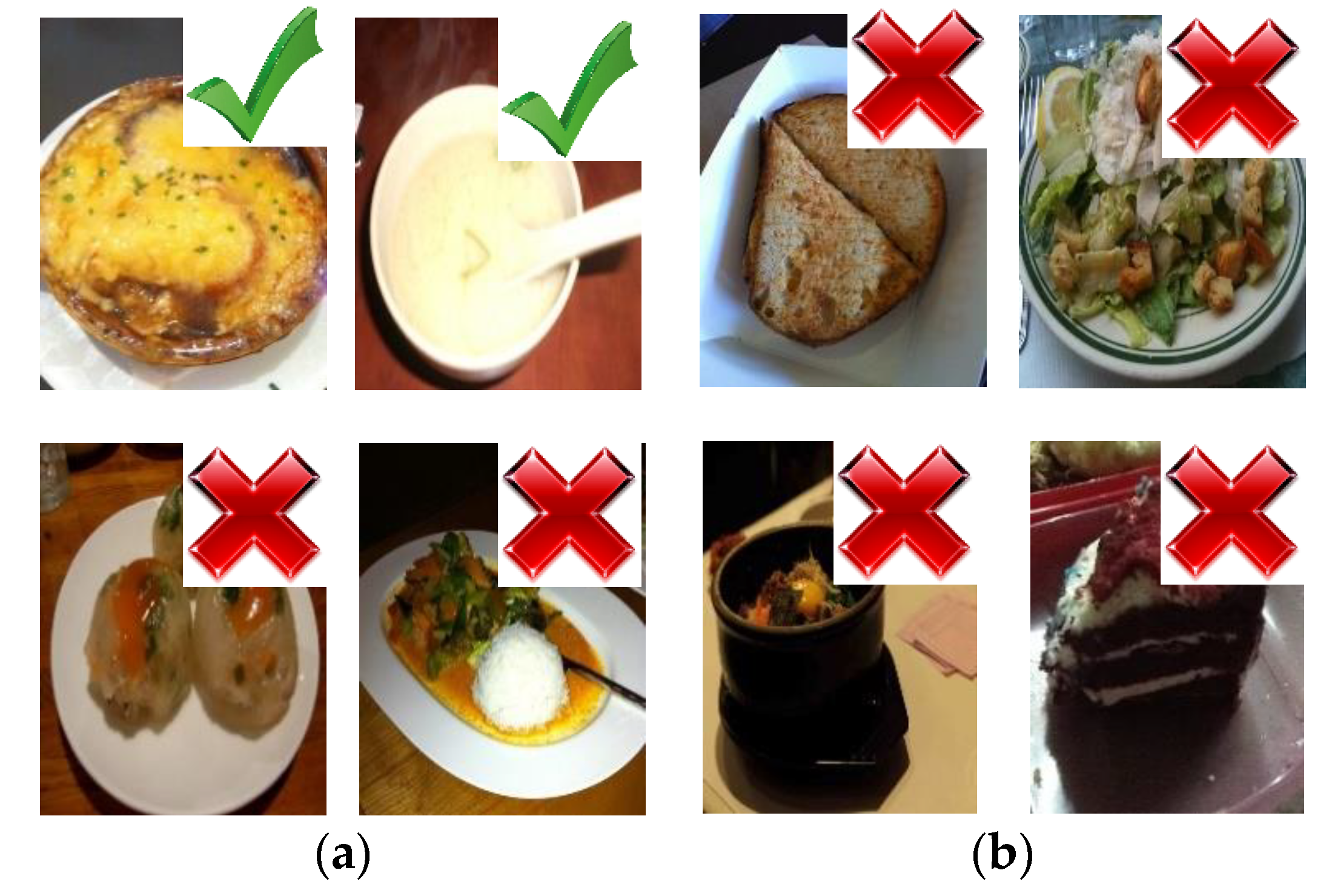
In the second set of experiments, we evaluate the performance of the SSNet framework using the off-the-shelf CNN local features. All the methods adopt the same settings as in the previous experiments. The proposed FV+SSNet yields an accuracy of 65.3% on PFID61 and 60.6% on Food-101, outperforming other two methods, MOP [8] and FC-CNN [36]. These results validate the effectiveness of our proposed method. According to the classification results, Figure 8 lists some sample images from the Food-101 dataset.

4.6. Limitations

In the previous sections, the performance of the SSNet has been discussed. Next, we will analyze its limitations. Compared with the traditional BoVW representation model, the introduction of the saliency detection and the weighted second-order pooling operation enhance the discriminative ability of the SSNet image representation. However, both of the introduced modules have their own limitations. In practical application, the parameter R a t i o s a l in Equation (33) is important, which determines the size of the selected regions of an image for building the image representation. An inappropriate parameter setting may have a negative effect on the classification results. So, if a target in the recognition task exists in the non-saliency regions, we should assign a large value to R a t i o s a l so that the target can be included in the selected region. At present, the setting for the parameter R a t i o s a l only depends on people’s prior experience. In the future, we hope to find a solution that can adjust this parameter adaptively.
In addition, the weighted second-order pooling operation increases the dimension of the final representation, which will consume more memory resources. To solve this problem, people can try the following three approaches: (1) adopting low-dimension local features; (2) adopting small size codebooks; and (3) reducing the dimension of the final representation vector by dimensionality reduction methods.

5. Conclusions

In order to deal with the burstiness problem of features and introduce high-order information for image representation, we have proposed a novel framework, named Salient Superpixel Network (SSNet), to learn the mid-level image representation. It can be regarded as an extension of the BoVW representation model to exploit both the saliency detection and the weighted second-order pooling technologies. Specifically, we first propose a fast saliency detection method to choose the regions with high saliency values for representing the image. As a result, the interference information in the background is alleviated effectively. Secondly, the weighted second-order pooling (WSOP) method is applied to perform the feature aggregation. Different from the existing average and max pooling method, the WSOP is capable of introducing the second-order statistical information and in the meantime, weakening the side effect of burstiness among the features. The experimental results on several benchmarks indicate that the proposed SSNet representation method achieves better or comparable performance with respect to the state-of-the-art method, which can serve as an effective image representation framework for image classification.

Author Contributions

Methodology, Z.J.; Project administration, F.W. and X.H.; Software, X.G. and L.X. All authors have read and agreed to the published version of the manuscript.

Funding

This research was funded by the National Key Research and Development Program of China (No. 2018YFA0704605), and the National Major Scientific and Technological Special Project during the Thirteenth Five-year Plan Period (No.2017ZX05064).

Conflicts of Interest

The authors declare no conflict of interest.

References

  1. Csurka, G.; Dance, C.; Fan, L.; Willamowski, J.; Bray, C. Visual categorization with bags of keypoints. In Proceedings of the Workshop on Statistical Learning in Computer Vision, European Conference on Computer Vision, Prague, Czech Republic, 11–14 May 2004; pp. 1–22. [Google Scholar]
  2. Krizhevsky, A.; Sutskever, I.; Hinton, G.E. ImageNet classification with deep convolutional neural networks. Commun. ACM 2017, 60, 84–90. [Google Scholar] [CrossRef]
  3. Yang, J.C.; Yu, K.; Gong, Y.H.; Huang, T. Linear Spatial Pyramid Matching Using Sparse Coding for Image Classification. In Proceedings of the IEEE Conference on Computer Vision and Pattern Recognition, Miami, FL, USA, 20–25 June 2009; Volumes 1–4, pp. 1794–1801. [Google Scholar]
  4. Wang, J.J.; Yang, J.C.; Yu, K.; Lv, F.J.; Huang, T.; Gong, Y.H. Locality-constrained Linear Coding for Image Classification. In Proceedings of the IEEE Conference on Computer Vision and Pattern Recognition, San Francisco, CA, USA, 13–18 June 2010; pp. 3360–3367. [Google Scholar]
  5. Jegou, H.; Douze, M.; Schmid, C.; Perez, P. Aggregating local descriptors into a compact image representation. In Proceedings of the IEEE Conference on Computer Vision and Pattern Recognition, San Francisco, CA, USA, 13–18 June 2010; pp. 3304–3311. [Google Scholar]
  6. Lowe, D.G. Distinctive image features from scale-invariant keypoints. Int. J. Comput. Vis. 2004, 60, 91–110. [Google Scholar] [CrossRef]
  7. Lazebnik, S.; Schmid, C.; Ponce, J. Beyond bags of features: Spatial pyramid matching for recognizing natural scene categories. In Proceedings of the IEEE Computer Society Conference on Computer Vision and Pattern Recognition, New York, NY, USA, 17–22 June 2006; pp. 2169–2178. [Google Scholar]
  8. Gong, Y.; Wang, L.; Guo, R.; Lazebnik, S. Multi-scale Orderless Pooling of Deep Convolutional Activation Features. In Proceedings of the European Conference on Computer Vision, Zurich, Switzerland, 6–12 September 2014; Volume 8695, pp. 392–407. [Google Scholar]
  9. Liu, L.; Shen, C.; van den Hengel, A. The Treasure beneath Convolutional Layers: Cross-convolutional-Iayer Pooling for Image Classification. In Proceedings of the Conference on Computer Vision and Pattern Recognition, Boston, MA, USA, 7–12 June 2015; pp. 4749–4757. [Google Scholar]
  10. Jegou, H.; Douze, M.; Schmid, C. On the burstiness of visual elements. In Proceedings of the IEEE Conference on Computer Vision and Pattern Recognition, Miami, FL, USA, 20–25 June 2009; Volume 4, pp. 1169–1176. [Google Scholar]
  11. Murray, N.; Jegou, H.; Perronnin, F.; Zisserman, A. Interferences in Match Kernels. IEEE Trans. Pattern Anal. Mach. Intell. 2017, 39, 1797–1810. [Google Scholar] [CrossRef] [PubMed] [Green Version]
  12. Russakovsky, O.; Lin, Y.; Yu, K.; Li, F.F. Object-Centric Spatial Pooling for Image Classification. In Proceedings of the European Conference on Computer Vision, Florence, Italy, 7–13 October 2012; Volume 7573, pp. 1–15. [Google Scholar]
  13. Angelova, A.; Zhu, S. Efficient object detection and segmentation for fine-grained recognition. In Proceedings of the IEEE Conference on Computer Vision and Pattern Recognition, Portland, OR, USA, 23–28 June 2013; pp. 811–818. [Google Scholar]
  14. Ji, Z.; Wang, J.; Su, Y.; Song, Z.; Xing, S. Balance between object and background: Object-enhanced features for scene image classification. Neurocomputing 2013, 120, 15–23. [Google Scholar] [CrossRef]
  15. Sharma, G.; Jurie, F.; Schmid, C. Discriminative Spatial Saliency for Image Classification. In Proceedings of the IEEE Conference on Computer Vision and Pattern Recognition, Providence, RI, USA, 16–21 June 2012; pp. 3506–3513. [Google Scholar]
  16. Murray, N.; Perronnin, F. Generalized Max Pooling. In Proceedings of the IEEE Conference on Computer Vision and Pattern Recognition, Columbus, OH, USA, 23–28 June 2014; pp. 2473–2480. [Google Scholar]
  17. Koniusz, P.; Yan, F.; Mikolajczyk, K. Comparison of mid-level feature coding approaches and pooling strategies in visual concept detection. Comput. Vis. Image Underst. 2013, 117, 479–492. [Google Scholar] [CrossRef]
  18. Carreira, J.; Caseiro, R.; Batista, J.; Sminchisescu, C. Free-Form Region Description with Second-Order Pooling. IEEE Trans. Pattern Anal. Mach. Intell. 2015, 37, 1177–1189. [Google Scholar] [CrossRef]
  19. Koniusz, P.; Yan, F.; Gosselin, P.H.; Mikolajczyk, K. Higher-Order Occurrence Pooling for Bags-of-Words: Visual Concept Detection. IEEE Trans. Pattern Anal. Mach. Intell. 2017, 39, 313–326. [Google Scholar] [CrossRef] [Green Version]
  20. Huang, D.; Zhu, C.; Wang, Y.; Chen, L. HSOG: A Novel Local Image Descriptor Based on Histograms of the Second-Order Gradients. IEEE Trans. Image Process. 2014, 23, 4680–4695. [Google Scholar] [CrossRef] [Green Version]
  21. Han, X.H.; Chen, Y.W.; Xu, G. High-Order Statistics of Weber Local Descriptors for Image Representation. IEEE Trans. Cybern. 2015, 45, 1180–1193. [Google Scholar] [CrossRef]
  22. Sanchez, J.; Perronnin, F.; Mensink, T.; Verbeek, J. Image Classification with the Fisher Vector: Theory and Practice. Int. J. Comput. Vis. 2013, 105, 222–245. [Google Scholar] [CrossRef]
  23. Li, P.; Lu, X.; Wang, Q. From Dictionary of Visual Words to Subspaces: Locality-constrained Affine Subspace Coding. In Proceedings of the IEEE Conference on Computer Vision and Pattern Recognition, Boston, MA, USA, 7–12 June 2015; pp. 2348–2357. [Google Scholar]
  24. Li, P.; Zeng, H.; Wang, Q.; Shiu, S.C.K.; Zhang, L. High-Order Local Pooling and Encoding Gaussians Over a Dictionary of Gaussians. IEEE Trans. Image Process. 2017, 26, 3372–3384. [Google Scholar] [CrossRef] [PubMed]
  25. Dalal, N.; Triggs, B. Histograms of oriented gradients for human detection. In Proceedings of the IEEE Computer Society Conference on Computer Vision and Pattern Recognition, San Diego, CA, USA, 20–26 June 2005; Volume 1, pp. 886–893. [Google Scholar]
  26. Liu, L.; Wang, L.; Liu, X. In Defense of Soft-assignment Coding. In Proceedings of the 2011 International Conference on Computer Vision, Barcelona, Spain, 6–13 November 2011; pp. 2486–2493. [Google Scholar]
  27. van Gemert, J.C.; Veenman, C.J.; Smeulders, A.W.M.; Geusebroek, J.M. Visual Word Ambiguity. IEEE Trans. Pattern Anal. Mach. Intell. 2010, 32, 1271–1283. [Google Scholar] [CrossRef] [PubMed] [Green Version]
  28. Boureau, Y.L.; Bach, F.; LeCun, Y.; Ponce, J. Learning Mid-Level Features For Recognition. In Proceedings of the IEEE Conference on Computer Vision and Pattern Recognition, San Francisco, CA, USA, 13–18 June 2010; pp. 2559–2566. [Google Scholar]
  29. Sicre, R.; Tasli, H.E.; Gevers, T. SuperPixel based Angular Differences as a mid-level Image Descriptor. In Proceedings of the International Conference on Pattern Recognition, Stockholm, Sweden, 24–28 August 2014; pp. 3732–3737. [Google Scholar]
  30. Yuan, J.; Wu, Y.; Yang, M. Discovery of collocation patterns: From visual words to visual phrases. In Proceedings of the IEEE Conference on Computer Vision and Pattern Recognition, Minneapolis, MN, USA, 17–22 June 2007; Volumes 1–8, pp. 1930–1938. [Google Scholar]
  31. Chatfield, K.; Simonyan, K.; Vedaldi, A.; Zisserman, A. Return of the Devil in the Details: Delving Deep into Convolutional Nets. arXiv 2014, arXiv:1405.3531. Available online: https://arxiv.org/abs/1405.3531 (accessed on 5 November 2014).
  32. Simonyan, K.; Zisserman, A. Very Deep Convolutional Networks for Large-Scale Image Recognition. arXiv 2014, arXiv:1409.1556. Available online: https://arxiv.org/abs/1409.1556 (accessed on 10 April 2015).
  33. Lin, T.Y.; Dollar, P.; Girshick, R.; He, K.; Hariharan, B.; Belongie, S. Feature Pyramid Networks for Object Detection. In Proceedings of the IEEE Conference on Computer Vision and Pattern Recognition, Honolulu, HI, USA, 21–26 July 2017; pp. 936–944. [Google Scholar]
  34. Ren, S.; He, K.; Girshick, R.; Zhang, X.; Sun, J. Object Detection Networks on Convolutional Feature Maps. IEEE Trans. Pattern Anal. Mach. Intell. 2017, 39, 1476–1481. [Google Scholar] [CrossRef]
  35. He, K.; Zhang, X.; Ren, S.; Sun, J. Deep Residual Learning for Image Recognition. In Proceedings of the IEEE Conference on Computer Vision and Pattern Recognition, Las Vegas, NV, USA, 27–30 June 2016; pp. 770–778. [Google Scholar]
  36. Razavian, A.S.; Azizpour, H.; Sullivan, J.; Carlsson, S. CNN Features off-the-shelf: An Astounding Baseline for Recognition. In Proceedings of the IEEE Conference on Computer Vision and Pattern Recognition, Columbus, OH, USA, 23–28 June 2014; pp. 512–519. [Google Scholar]
  37. Tang, P.; Wang, X.; Shi, B.; Bai, X.; Liu, W.; Tu, Z. Deep FisherNet for Image Classification. IEEE Trans. Neural Netw. Learn. Syst. 2019, 30, 2244–2250. [Google Scholar] [CrossRef]
  38. Arandjelovic, R.; Gronat, P.; Torii, A.; Pajdla, T.; Sivic, J. NetVLAD: CNN Architecture for Weakly Supervised Place Recognition. IEEE Trans. Pattern Anal. Mach. Intell. 2018, 40, 1437–1451. [Google Scholar] [CrossRef] [Green Version]
  39. Oquab, M.; Bottou, L.; Laptev, I.; Sivic, J. Learning and Transferring Mid-Level Image Representations using Convolutional Neural Networks. In Proceedings of the IEEE Conference on Computer Vision and Pattern Recognition, Columbus, OH, USA, 23–28 June 2014; pp. 1717–1724. [Google Scholar]
  40. Li, Y.; Liu, L.; Shen, C.; van den Hengel, A. Mining Mid-level Visual Patterns with Deep CNN Activations. Int. J. Comput. Vis. 2017, 121, 344–364. [Google Scholar] [CrossRef] [Green Version]
  41. Donggeun, Y.; Sunggyun, P.; Joon-Young, L.; In So, K. Multi-scale pyramid pooling for deep convolutional representation. In Proceedings of the IEEE Conference on Computer Vision and Pattern Recognition Workshops, Boston, MA, USA, 7–12 June 2015; pp. 71–80. [Google Scholar]
  42. Liang, Z.; Yali, Z.; Shengjin, W.; Jingdong, W.; Qi, T. Good Practice in CNN Feature Transfer. arXiv 2016, arXiv:1604.00133. Available online: https://arxiv.org/abs/1604.00133 (accessed on 1 April 2016).
  43. Azizpour, H.; Razavian, A.S.; Sullivan, J.; Maki, A.; Carlsson, S. From generic to specific deep representations for visual recognition. In Proceedings of the IEEE Conference on Computer Vision and Pattern Recognition, Boston, MA, USA, 7–12 June 2015; pp. 36–45. [Google Scholar]
  44. Liu, L.; Shen, C.; Wang, L.; van den Hengel, A.; Wang, C. Encoding High Dimensional Local Features by Sparse Coding Based Fisher Vectors. In Advances in Neural Information Processing Systems; NIPS: Montreal, QC, Canada, 2014; Volume 27, pp. 1143–1151. [Google Scholar]
  45. Zeiler, M.D.; Fergus, R. Visualizing and Understanding Convolutional Networks. In Proceedings of the European Conference on Computer Vision, Zurich, Switzerland, 6–12 September 2014; Volume 8689, pp. 818–833. [Google Scholar]
  46. Agrawal, P.; Girshick, R.; Malik, J. Analyzing the Performance of Multilayer Neural Networks for Object Recognition. In Proceedings of the European Conference on Computer Vision, Zurich, Switzerland, 6–12 September 2014; Volume 8695, pp. 329–344. [Google Scholar]
  47. Zhang, L.; Gao, Y.; Xia, Y.; Dai, Q.; Li, X. A Fine-Grained Image Categorization System by Cellet-Encoded Spatial Pyramid Modeling. IEEE Trans. Ind. Electron. 2015, 62, 564–571. [Google Scholar] [CrossRef]
  48. Celikkale, B.; Erdem, A.; Erdem, E. Visual Attention-driven Spatial Pooling for Image Memorability. In Proceedings of the IEEE Conference on Computer Vision and Pattern Recognition, Portland, OR, USA, 23–28 June 2013; pp. 976–983. [Google Scholar]
  49. Zhang, L.; Hong, R.; Gao, Y.; Ji, R.; Dai, Q.; Li, X. Image Categorization by Learning a Propagated Graphlet Path. IEEE Trans. Neural Netw. Learn. Syst. 2016, 27, 674–685. [Google Scholar] [CrossRef]
  50. Perronnin, F.; Sanchez, J.; Mensink, T. Improving the Fisher Kernel for Large-Scale Image Classification. In Proceedings of the European Conference on Computer Vision, Crete, Greece, 5–11 September 2010; Volume 6314, pp. 143–156. [Google Scholar]
  51. Tuzel, O.; Porikli, F.; Meer, P. Region covariance: A fast descriptor for detection and classification. In Proceedings of the European Conference on Computer Vision, Graz, Austria, 7–13 May 2006; Volume 3952, pp. 589–600. [Google Scholar]
  52. Xu, L.; Ji, Z.; Dempere-Marco, L.; Wang, F.; Hu, X. Gestalt-grouping based on path analysis for saliency detection. Signal Process. Image Commun. 2019, 78, 9–20. [Google Scholar] [CrossRef]
  53. Tu, W.C.; He, S.; Yang, Q.; Chen, S.Y. Real-Time Salient Object Detection with a Minimum Spanning Tree. In Proceedings of the IEEE Conference on Computer Vision and Pattern Recognition, Las Vegas, NV, USA, 27–30 June 2016; pp. 2334–2342. [Google Scholar]
  54. Achanta, R.; Shaji, A.; Smith, K.; Lucchi, A.; Fua, P.; Suesstrunk, S. SLIC Superpixels Compared to State-of-the-Art Superpixel Methods. IEEE Trans. Pattern Anal. Mach. Intell. 2012, 34, 2274–2281. [Google Scholar] [CrossRef] [Green Version]
  55. Dong, Z.; Jia, S.; Zhang, C.; Pei, M.; Wu, Y. Deep Manifold Learning of Symmetric Positive Definite Matrices with Application to Face Recognition. In Proceedings of the Thirty-First AAAI Conference on Artificial Intelligence, San Francisco, CA, USA, 4–9 February 2017; pp. 4009–4015. [Google Scholar]
  56. Arsigny, V.; Fillard, P.; Pennec, X.; Ayache, N. Geometric means in a novel vector space structure on symmetric positive-definite matrices. Siam J. Matrix Anal. Appl. 2007, 29, 328–347. [Google Scholar] [CrossRef] [Green Version]
  57. Vedaldi, A.; Fulkerson, B. VLFeat: An open and portable library of computer vision algorithms. In Proceedings of the 18th ACM international conference on Multimedia, Firenze, Italy, 21–25 October 2010; pp. 1469–1472. [Google Scholar]
  58. Vedaldi, A.; Lenc, K. Matconvnet: Convolutional neural networks for matlab. In Proceedings of the 23rd ACM International Conference on Multimedia; ACM: New York, NY, USA, 2015; pp. 689–692. [Google Scholar]
  59. Chen, M.; Dhingra, K.; Wu, W.; Yang, L.; Sukthankar, R.; Yang, J. PFID: Pittsburgh fast-food image dataset. In Proceedings of the 16th IEEE International Conference on Image Processing, Piscataway, NJ, USA, 7–10 November 2009; pp. 289–292. [Google Scholar]
  60. Bossard, L.; Guillaumin, M.; Van Gool, L. Food-101–mining discriminative components with random forests. In Proceedings of the European Conference on Computer Vision, Zurich, Switzerland, 6–12 September 2014; pp. 446–461. [Google Scholar]
  61. Bin-Bin, G.; Xiu-Shen, W.; Jianxin, W.; Weiyao, L. Deep spatial pyramid: The devil is once again in the details. arXiv 2015, arXiv:1504.05277. Available online: https://arxiv.org/abs/1504.05277 (accessed on 23 April 2015).
Figure 1. Observing the burstiness property of the features in a natural image. (a) An image with the object in a red bounding box; (b) The visualization of the Dense SIFT descriptors sampled from Figure 1a (note that Figure 1b just demonstrates a part of the descriptors in the background and each column corresponds to a descriptor. The features of the object are rearranged and placed in the right red bounding box).
Applsci 10 00140 g001
Figure 2. The overall architecture of the proposed representation model and its key modules. The two red bounding boxes denote the proposed modules. The left one denotes the saliency detection method and the right one indicates the weighted second-order pooling module.
Applsci 10 00140 g002
Figure 3. A depiction of the process of extracting convolutional neural networks (CNN) local features from a convolutional layer. The star denotes the spatial position of the corresponding feature.
Applsci 10 00140 g003
Figure 4. An illustration of the two-stage minimum bottleneck distance transform. In (a), only the distance values of the seed nodes are set to 0. (b) demonstrates the bottom–up updating process from the leaves, and the changed values are labeled in yellow color. (c) shows the top–down traversal process from the root node.
Applsci 10 00140 g004
Figure 5. Illustration of the pipeline for generating the Salient Superpixel Network (SSNet) mid-level image representation.
Applsci 10 00140 g005
Figure 6. Saliency maps for the images from VOC 2007 and 15-Scene. (a) Saliency maps for images taken from Pascal VOC 2007; (b) Saliency maps for images taken from 15-Scene.
Applsci 10 00140 g006
Figure 7. Performance of the improved LLC representation with different saliency region ratios. This figure illustrates the classification accuracy of LLC representation, formed by the LLC encoding method conducting on different numbers of saliency regions, on the benchmark datasets.
Applsci 10 00140 g007
Figure 8. Some sample images from the Food-101 dataset. (a) These four images are selected to build the SSNet representation using the Dense SIFT features. (b) These four images are selected to build the SSNet representation using the CNN local features. The check mark indicates that this image can be recognized correctly by our proposed method, and the cross indicates that our method cannot recognize this image correctly.
Applsci 10 00140 g008
Table 1. Classification accuracy (MAP in %) of the weighted second-order pooling scheme integrating with the bag-of-visual-words (BoVW) baseline encoding methods. FV: Fisher Vector, VLAD: Vector of Locally Aggregated Descriptor, WSOAP: weighted second-order average pooling, WSOMP: weighted second-order pooling.
PASCAL VOC 2007Caltech 101Caltech 25615-Scene
ScSPM [3]51.973.237.580.3
LLC [4]58.775.446.382.0
FV [22]61.877.852.185.3
VLAD [5]55.377.648.983.2
SC + WSOAP63.180.147.385.7
SC + WSOMP64.981.951.886.1
LLC + WSOAP69.882.758.287.4
LLC + WSOMP71.383.160.387.9
FV + WSOAP72.486.166.189.6
FV + WSOMP73.587.569.991.0
VLAD + WSOAP69.684.261.686.7
VLAD + WSOMP72.185.663.288.2
Table 2. Classification accuracy (MAP in percentage) of the SSNet framework integrating with different BoVW baselines.
PASCAL VOC 2007Caltech 101Caltech 25615-Scene
ScSPM [3]51.973.237.580.3
LLC [4]58.775.446.382.0
FV [22]61.877.852.185.3
VLAD [5]55.377.648.983.2
SC + SSNet(max)66.583.353.187.2
LLC + SSNet(max)73.785.061.988.7
FV + SSNet(max)76.189.772.590.6
VLAD + SSNet(max)74.287.365.089.4
Table 3. Comparison with the baselines and state-of-the-art methods based on CNN local features (MAP in percentage).
PASCAL VOC 2007Caltech 101Caltech 25615-Scene
BaselineFC-CNN [36]84.389.781.390.2
CL-FV85.186.179.590.5
SOA MethodsMOP [8]85.591.885.492.7
MPP [41]88.093.787.394.1
DSP [32]88.694.784.291.1
MS-DSP [61]89.395.185.591.8
OursFV + SSNet(max)89.695.387.695.7
Table 4. Comparison of different image encoding methods using Dense SIFT, off-the-shelf CNN features on PFID61 and Food-101 datasets (MAP in percentage).
FeaturesMethodsPFID61Food-101
Dense SIFTFV [22]40.238.9
FV (using MASK)42.9NA
FV + WSOMP55.851.6
FV + SSNet57.152.4
Off-the-shelf CNN featuresFC-CNN [36]48.254.1
MOP [8]61.759.7
FV + SSNet65.360.6