Article

Effect of Track Irregularities on the Response of Two-Way Railway Tracks

Department of Civil and Environmental Engineering, Hanyang University, Seoul 04763, Korea
*
Author to whom correspondence should be addressed.
Appl. Sci. 2020, 10(1), 11; https://doi.org/10.3390/app10010011
Submission received: 15 November 2019 / Revised: 13 December 2019 / Accepted: 15 December 2019 / Published: 18 December 2019
(This article belongs to the Section Civil Engineering)

Abstract

:
In predicting the response of track from a moving train only one track is generally considered. However, the effect of ground vibrations from one track and its effect on the nearby tracks has not been studied completely. Therefore, in the present paper, the effect of track irregularities and speed on the prediction of two-way tracks response is investigated. For this purpose, a three-dimensional dynamic finite element (FE) model capable of simulating interactions between the train and track by using a nonlinear hertz contact method was developed. The model uses tensionless stiffness between the wheel and rail to couple them. The model components including the sleeper, ballast, and soil domain are represented by solid brick elements. The rails are modeled as 3D Euler–Bernoulli beam elements. An iterative numerical algorithm was established for the integrations of the train and track interface. A comparative analysis was performed at various speeds and rail surface irregularity wavelengths. With the increase in speed, the results showed a significant increase in the adjacent tracks response and can induce much larger track vibrations at high frequency.

1. Introduction

Railways are a paramount and economical means for mass transportation and offer a suitable alternative to traffic congestion. However, in populated areas, ground vibrations induced by the moving trains is problematic. To examine this problem, various train–track models have been proposed to study the generation of ground vibrations and their propagation due to moving loads. Most of the early train–track models to study the effect of moving loads were based on analytical and semi-analytical methods [1,2,3,4]. However, these methods are hard to formulate, limited to the specific types of problems, consider many simplified assumptions and difficult to implement to study the wave propagation due to moving loads. Therefore, a better understanding of the ground vibrations and wave propagation during the design and the construction of such facilities is highly desirable [5].
To study the ground vibration due to moving load, Xia et al. [6] developed a theoretical train–track–subsoil interaction model and also considered track irregularities. This interaction model takes account of quasi-static as well as dynamic excitation between the vehicle and track. The results showed that the track unevenness could significantly increase the vibrations in the ground at a given speed.
With the progress of computer technology, more sophisticated methods such as boundary element method (BEM), finite element method (FEM) and combined or hybrid methods have been introduced to solve ground vibration problems. Many researchers considered BEM [7,8,9] or combined methods [10,11,12,13,14] to study the effect of moving train on ground vibration and surrounding structures. Generally, these methods are mostly formulated in the frequency domain because of computational efficiency. However, these methods are limited to linear problems and become inconvenient for solving complex geometries.
The FEM precisely predict the ground vibrations and can give a replica of engineering insight of operational conditions. The FEM can easily solve nonlinear problems with complex geometries. El Kacimi et al. [15] used three-dimensional finite element (FE) coupled train–track model to predict the track vibration at high speed. Their findings revealed that a series of waves radiating from the loading point formed a Mach cone, which caused the loss of symmetry in ground vibration at critical speed. The effect of rail surface irregularities was not considered in this study which is the main source of the increase in ground vibration in the train–track interaction problem. Moreover, to simplify the problem it was assumed that the track has symmetry all along the track. A half finite element domain with a single rail, half of the track and ground along the track was modeled to study the ground vibration due to moving load. This assumption is not useful while considering track irregularities. Furthermore, a lot of FEM based parametric studies have been carried out to investigate the effect of moving load under different track and ground conditions [16,17,18,19,20,21,22].
The impact of train induced vibrations on adjacent structures and attenuation of ground vibration was studied by many researchers (e.g., [23,24,25,26,27,28]). In these studies, only one track or symmetry along the track (only one single rail) is considered to predict the track and ground vibrations due to moving loads. In real-world practice, two-way tracks are mostly constructed; and one track can easily be affected by the ground-borne vibrations induced by a moving train on the nearby track which has been ignored in previous studies. Therefore, for two-way tracks, the excitation on both tracks due to moving trains should be considered. To this end, a better model reflecting the overall responses, due to separate excitation on two tracks and the effect of waves propagating from one track to the other track needs to be studied.
In this study, a model comprising three-dimensional soil domain and two-way track to investigate the effect of radiating waves from one track to the nearby track is developed. This model also considers the nonlinear train–track interaction and the rail–sleeper–ballast–soil interaction. Moreover, Lysmer boundary is considered to avoid the reflection of the wave from the soil domain. Finally, the results of this numerical simulation and the effect of different classes of irregularities on tracks at different speeds are discussed.

2. Train-Track-Soil Interaction Model

A time-domain Train-Track-Soil interaction model was developed to study the effect of different level of track irregularities on the response of two adjacent railway tracks. In this study, three separate models are considered (1) train model, (2) track and soil model and (3) track irregularities. The train was modeled as a quarter train model [15]. A track consisting of two rails was placed on sleepers that were connected by rail-pads. The rails were modeled as 3D-beams and rail pads as distributed spring-dashpot elements, which transmit all the forces caused by the moving train to the track–soil system. The other parts of the track (i.e., sleeper and ballast) and soil domain were modeled as solid elements. Lysmer and Kuhlmeyeer boundary condition was incorporated to prevent the reflection of stress waves from the edges of the domain [29]. Furthermore, Non-linear Hertz contact theory was utilized to couple train and track. The track irregularity was modeled as a stationary Gaussian random process based on power spectral density function. A detailed explanation of each model is given as follows:

2.1. Train Model

A quarter train model was used to simulate the vehicle body. The quarter train model consists of a quarter car body, half bogie, and a wheel. Each of these components is modeled as a rigid mass connected by two suspension systems (i.e., primary and secondary suspension systems). Figure 1 illustrates a schematic layout of the quarter train model, where the masses of quarter of a car body, half of a bogie and a wheel are denoted by m w 1 , m w 2 and m w 3 respectively. The primary suspension system which connects the wheel and bogie has stiffness k w 2 and damping c w 2 the secondary suspension system connects bogie and car body has stiffness k w 1 and damping c w 1 . K H presents the Hertz contact spring. The equations of motion for the given train model are derived as:
M v ¨ w ( t ) + C v ˙ w ( t ) + K v w ( t ) = F ( t ) ,
where M , C and K are the mass, damping and stiffness matrices of the train system, and F is the load vector. Equation (1) can be written in expanded form as:
[ m w 1 0 0 0 m w 2 0 0 0 m w 3 ] { v ¨ w 1 v ¨ w 2 v ¨ w 3 } + [ c w 1 c w 1 0 c w 1 c w 1 + c w 2 c w 2 0 c w 2 c w 2 ] { v ˙ w 1 v ˙ w 2 v ˙ w 3 } + [ k w 1 k w 1 0 k w 1 k w 1 + k w 2 k w 2 0 k w 2 k w 2 ] { v w 1 v w 2 v w 3 }          = { m w 1 g m w 2 g m w 3 g } + { 0 0 F w / r }  
In which:
m w 1 = m ¯ w 1 / 8
m w 2 = m ¯ w 2 / 4 ,
where m ¯ w 1 , m ¯ w 2 and m w 3 are the masses of car body, bogie, and a wheel, respectively and v w 1 , v w 2 and v w 3 are the vertical displacements of the car, bogie, and wheel, respectively.
The coupling of wheel and rail can be obtained through the interaction forces between the wheel and rail and is given [15] as:
F w / r = { K H ( v w 3 v r i r r ) 3 2 ,   if   v w 3 ( v r i r r ) < 0 ,   0 ,           if   v w 3 ( v r i r r ) > 0 ,
where F w / r is the interaction force between wheel and rail, K H is the contact spring constant, v w 3 and v r are the vertical displacements of the respective wheel and rail at the point of contact, and i r r is the surface irregularity of the rail surface.

2.2. Track–Soil Model

To investigate the ground vibration due to a moving train, the parts of the track such as the sleeper and ballast, and soil domain are modeled as a homogeneous material. The rail is modeled as a 3D Euler–Bernoulli beam. Three-dimensional (3D) FEM is adapted to model the track and soil. The geometry, material damping, radiational damping and mesh size of the model are the critical parameters. The track (i.e., sleeper and ballast) and soil are modeled as brick elements. The governing equation of motion for track and soil is given as:
M ˜ v ¨ ( t ) + C ˜ v ˙ ( t ) + K ˜ v ( t ) = F ˜ ( t ) ,
where M ˜ , C ˜ and K ˜ are the total mass, damping and stiffness matrices of complete track and soil model which includes rail, sleepers, ballast and soil domain.
M ˜ = M t s + M r
K ˜ = K t s + K r
C ˜ = C t s + C r + C s , p ,
where   M ts   and   M r are the mass matrices of track–soil and rail, respectively; K ts ,     K r are the stiffness matrices of track–soil and rail, respectively, and C ts ,   C r are the material damping matrices of track/soil and rail respectively. Radiational damping coefficient is presented as C s , p .
M ts = V e   ρ N T N dV
  K ts = V e   B T c B dA ,  
where ρ is the density of respective material and N the shape function field. In the stiffness matrix, c is the matrix of material constant and B is the strain matrix.
The Rayleigh damping is used to calculate the material damping, a linear combination of the mass matrix and stiffness matrix.
C ts = α ts M ts + β ts K ts
  C r = α r M r + β r K r ,  
where α ts ,   β ts   ,   α r   and   β r are the Rayleigh damping coefficients. Material damping calculated by this method is frequency dependent and can be predicted using Equations (12) and (13), for the constant damping ratio, the scalar values of the coefficients in the linear combination can be calculated as given in [30].
The Lysmer and Kuhlmeyeer model [29] for infinite media is used to formulate the artificial boundary. The Lysmer boundary is a way to avoid the full reflection of waves by the domain boundaries. This is critical because reflected waves may cause resonance in the domain that does not actually exist in reality. The implementation of this kind of boundary is very easy and compatible with finite element modeling as it is a simple connection of dampers to all degrees of freedom of soil boundary nodes and the other end is fixed. The radiational damping coefficient of these dampers can be calculated by Equation (14).
C s , p = ρ AV s , p ,
where A is the cross-sectional area of the element, ρ is the mass density and V s , p are the wave velocity depending upon the type of wave (shear wave velocity V s or compressional wave velocity V p ).
A wide range of frequencies are excited in the wave propagation problems. To solve this problem easily is to select a high cutoff frequency to get an accurate solution. Selecting the mesh size of elements is very important for defining the proper time step, correct wave front propagation through space from one point to the other, and stability of the solution. The Courant–Friedrichs–Lewy (CFL) method has been used as in [31].
Δ h λ 4 = V 4 f max
Δ t < Δ h V   ,
where Δ h is maximum nodes spacing; λ is the smallest wavelength; V is the lowest wave velocity of interest; f max highest frequency present in the simulation; and Δ t is the time step.

2.3. Track Irregularities

The main source of ground vibrations is the loads of the wheels acting on the rail. The track irregularities are considered to increase the ground vibrations. In the present study, the track irregularities are numerically generated using the power spectral density function (PSD), developed by the USA Federal Railway Administration [32], and is given as:
S ( ϕ k ) = A ϕ 2 2 ( ϕ 2 k + ϕ 2 1 ) ϕ 4 k ( ϕ 2 k + ϕ 2 2 ) ,
where A, ϕ 1 and ϕ 2 are the constants defined in the actual measurement depending on the type of irregularity and rail quality. According to the practice by the Federal Railway Administration, USA, the level of track irregularities is categorized into six classes ranging from class1 (bad quality) to class6 (good or finest) [33]. The random vertical track irregularities i r r are modeled as a stationary Gaussian random process based on the PSD function and can be written as:
i r r ( y ) = k = 1 N k a k cos ( ϕ k y + θ k )
a k = 2 S ( ϕ k ) Δ ϕ
ϕ k = ϕ min + ( k 0.5 ) Δ ϕ
Δ ϕ = ϕ max ϕ min N k   ,
where a k is the amplitude of the wave, ϕ k is the circular spatial frequency within the range of upper ( ϕ max ) and lower ( ϕ min ) limits of route frequency, θ k is the random phase angle with a uniform distribution between 0 and 2 π , N k represents the number of harmonic functions, and y is the global coordinates along the rail.

3. Numerical Analysis Procedure

The equation of motion for train Equation (1) and the equation of motion of track and soil Equation (6) are coupled by the loads of the train due to its weight and interaction forces { F w / r } . The interaction forces depend on the position of the wheel on the rail, track irregularity, and time-dependent displacement of the rail. To integrate the two sub-systems (i.e., train and track–soil), an iterative scheme has been used which considers the contact force equilibrium as given in [34]. This iterative method also incorporates the Newmark integration method to solve the coupled train–track–soil dynamic system equations. The complete algorithm is given as follows:
Step 1: at first time step and iteration (i = 1), train responses { v w } i t , { v ˙ w } i t   and { v ¨ w } i t and track responses { v } i t , { v ˙ } i t   and { v ¨ } i t are assumed initially as zero.
Step 2: after first time step, the second iteration (i + 1) starts with the computation of the interaction force vector of all wheels { F w / r } i + 1 t + Δ t . The vertical contact forces of k   -th wheel can be evaluated from the last known responses of the wheel and rail at the position of contact by using equation Equation (5).
Step 3: this vertical contact forces with gravity loads of train given in Equation (2) are applied on rail as external loads. The track/soil responses at (i + 1) iteration with the time step (t + Δt) are computed by the following equations.
( [ K ] + a 1 [ M ] + a 2 [ C ] ) { v } t + Δ t = { F ( t ) } t + Δ t + [ M ] ( a 1 { v } t + a 3 { v ˙ } t a 4 { v ¨ } t ) + [ C ] ( a 2 { v } t + a 5 { v ˙ } t + a 6 { v ¨ } t )
{ v ˙ } t + Δ t = a 1 ( { v } t + Δ t { v } t ) a 5 { v ˙ } t a 6 { v ¨ } t
{ v ¨ } t + Δ t = a 1 ( { v } t + Δ t { v } t ) a 3 { v ˙ } t a 4 { v ¨ } t
Step 4: after getting the response of track/soil at a given time step, update the rail responses in Equation (5) at every position of wheels on rails defined as { v } i + 1 t + Δ t . Before moving to the next iteration, the convergence of the solution must be checked by the following equation.
{ v } i + 1 t + Δ t { v } i t + Δ t { v } i + 1 t + Δ t ε ,
where the { v } i + 1 t + Δ t , { v } i t + Δ t are the displacements of track at present and previous iterations and ε is the specified tolerance. If the convergence criterion is satisfied, return to the initial iteration (or Step 2) for the next time step otherwise move to step 5.
Step 5: if the convergence criterion is not satisfied, take the rail displacement at a given time { v r } from { v } i + 1 t + Δ t and calculate { F w / r } i + 1 t + Δ t by using Equation (5). Then, apply it on wheels as external force and obtained { v w } i + 1 t + Δ t , { v ˙ w } i + 1 t + Δ t and { v ¨ w } i + 1 t + Δ t by solving equations Equations (22)–(24). Now take { v w 3 } from { v w } i + 1 t + Δ t and turn to step 2 for the next iteration.

4. Numerical Results and Discussions

4.1. Numerical Validation

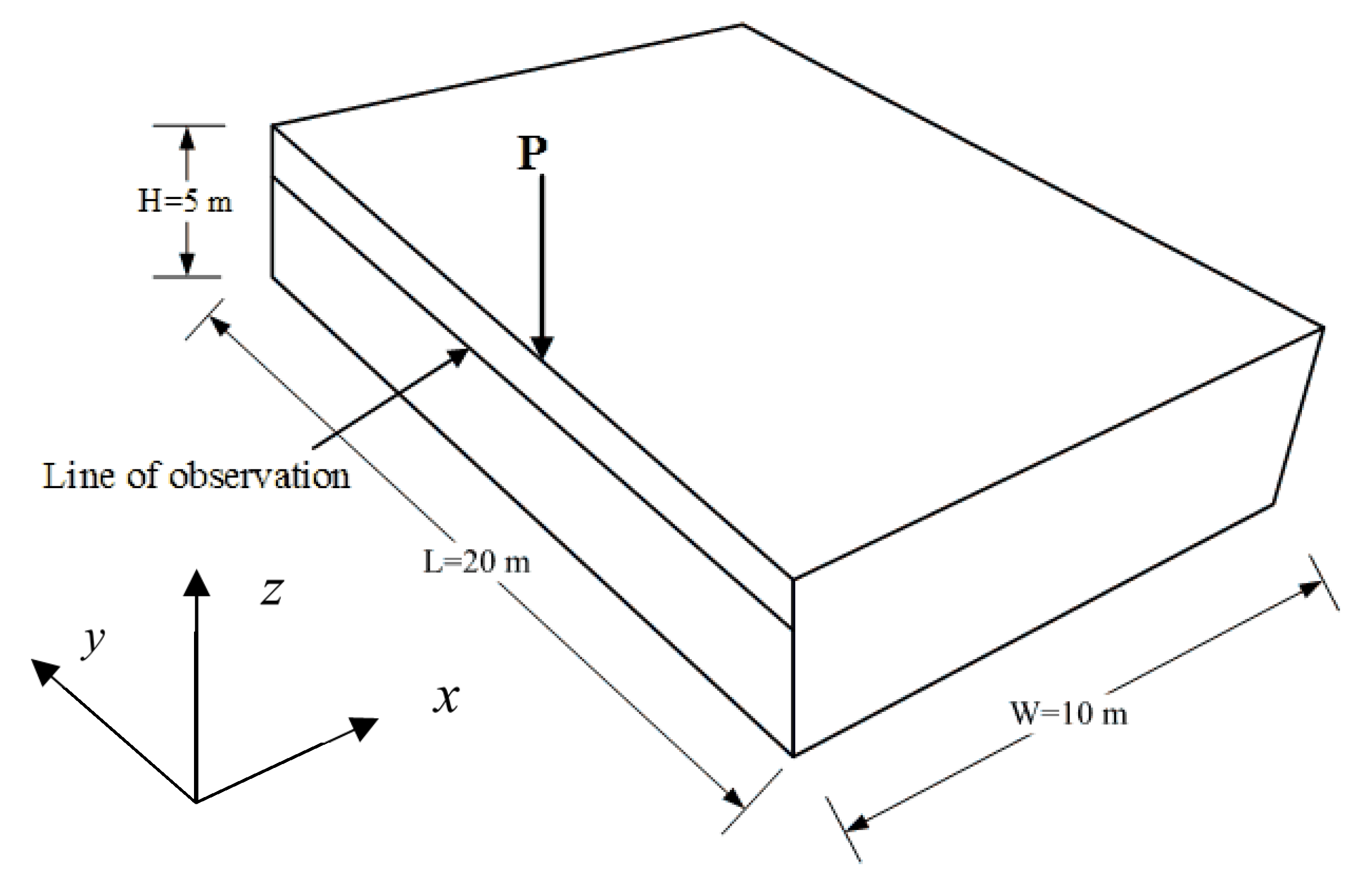
In this section, a three-dimensional finite element model (FEM) is developed for the analysis of the soil domain. The accuracy of the developed FE model is verified against the Boussinesq’s solution [35]. The constant vertical point load is applied to the soil domain with the dimensions 10 × 20 × 5 m. The properties of the domain are: Elastic modulus E = 0.11 GPa and Poisson’s ratio υ = 0.45. The vertical point load P of magnitude 20 kN is applied on the boundary of the soil domain as shown in Figure 2. The boundary along y z -plane is fixed in x direction to present the symmetrical boundary condition to validate the results of the soil domain with Boussinesq’s solution. Figure 3 illustrates the comparison between numerical and analytical displacements at the line of observation. The longitudinal and vertical displacements obtained by analytical and numerical methods are in close agreement, as shown in Figure 3a,b, respectively.

4.2. Effect of Train Speed and Track Irregularities

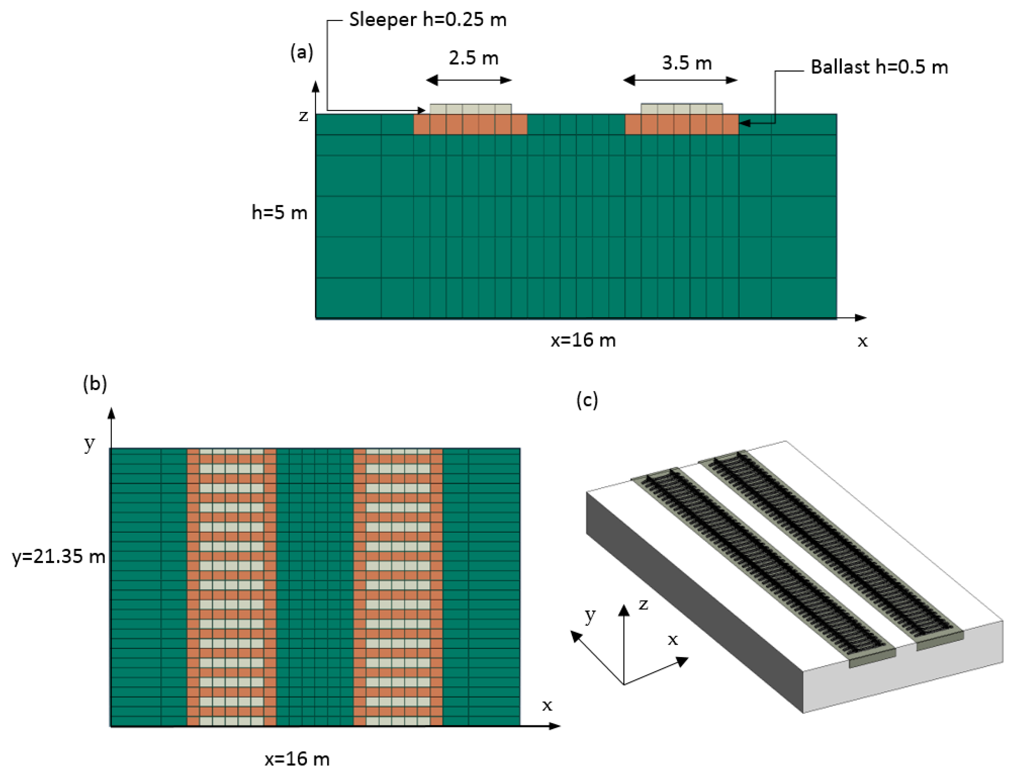
After validating the results of the soil model against Boussinesq’s solution, the train is modeled as a quarter train model. Figure 4 presents the configuration of the train on one rail. Table 1 shows the properties of the quarter train model. Track with sleepers at a spacing of 0.7 m centers with dimensions 2.5 m × 0.35 m × 0.25 m is considered. The rail was modeled using a beam element for which the properties are given in Table 2. The track and soil were modeled as three-dimensional solid elements. The depth of the domain is taken to 5 m and the distance between the two tracks is 6.5 m. Table 3 summarizes the properties of the track and soil. Rail-pads are represented by a combination of a spring-damper system to combine the rails and sleepers. The profile of the analyzing domain is shown in Figure 5.
In this paper, only one train car was considered to generalize the response of ground under loadings due to different levels of track irregularities on two tracks. Various experimental trials were carried out for different speeds at 30 m/s, 40 m/s, 50 m/s and 60 m/s, to study the effect of track quality on ground vibrations. Six (06) classes or levels of track irregularities were selected and calculated using the numerical generation method based on the PSD function. Table 4 shows the six track classes and the values of their parameters A, ϕ 1 and ϕ 2 .

4.3. Track Dynamic Response

A simulation tool for the dynamic analysis of the coupled train–track–soil system is developed in MATLAB. In order to investigate the effect of various levels of track irregularities on two-way train tracks responses, two (02) different analysis cases were considered as follows:
  • Train is considered only on right track (no train on left track)
  • Trains on both tracks, but moving in the opposite direction
Each case is further consisting of sub-cases depend upon the moving train and track condition as given in Table 5.

4.3.1. Case 01

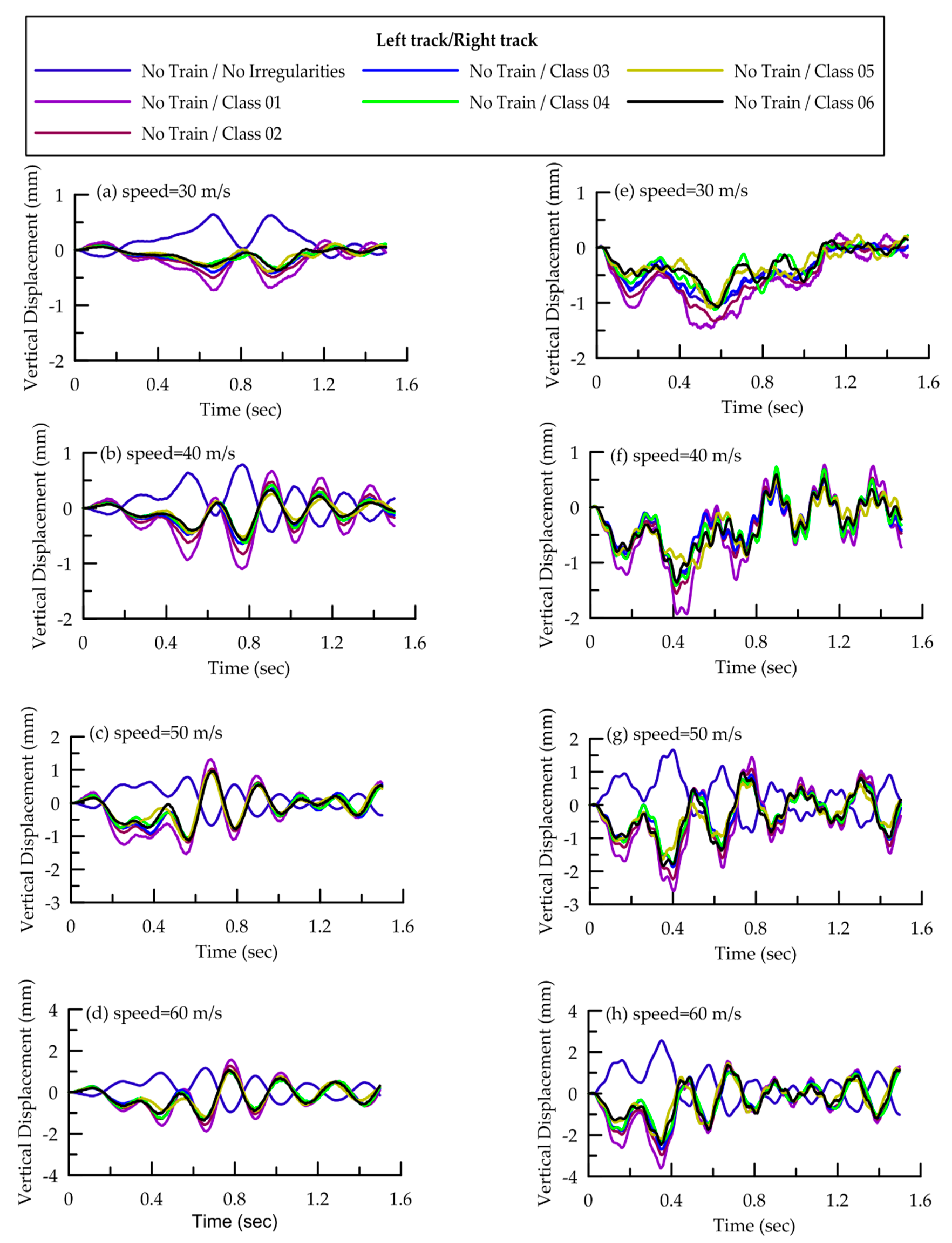
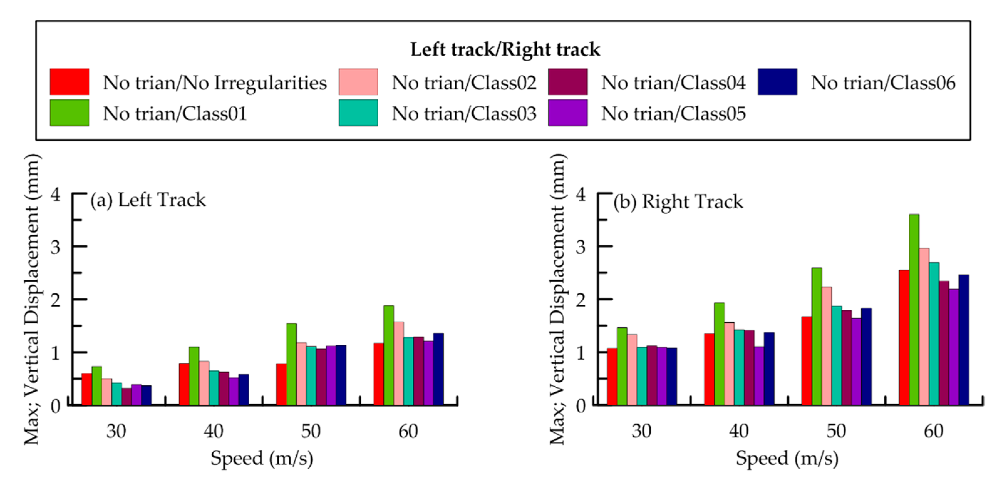
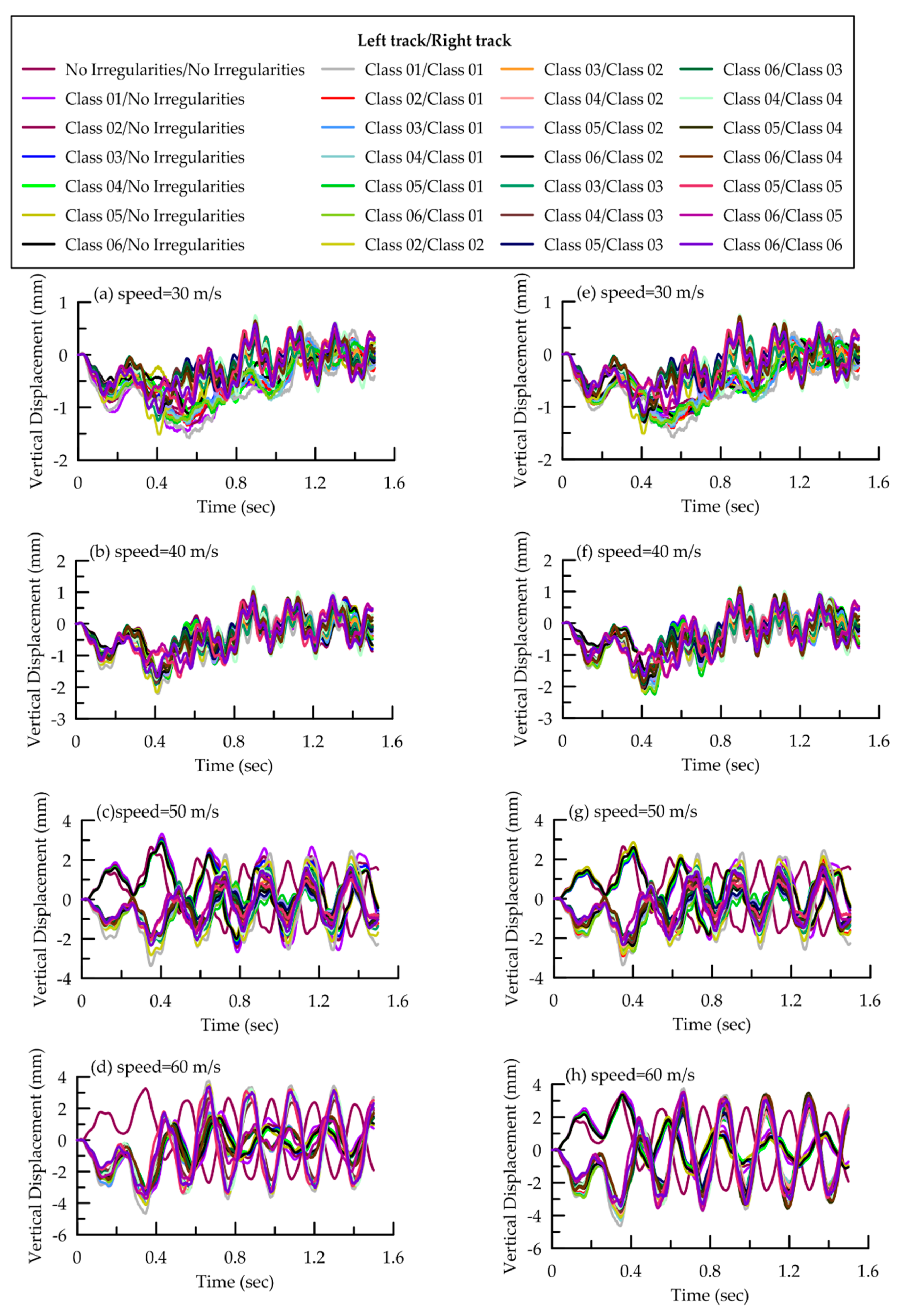
To get the general effect of moving train on one track and its effect on the adjacent track, it was considered that the train is moving only on right track, and there is no train moving on the left track. For analysis at different speeds, seven different conditions for the track were considered (one with no irregularities and six different levels of irregularities). The track irregularities were calculated by using the PSD function which is considered as input for train pass-by simulations that are the source from the track. The numerical method explained in Section 3 was used to investigate the effect of different interface conditions between the train and track due to different levels of track irregularities. Vertical displacements were obtained from the above-mentioned track conditions and at different speeds are plotted in Figure 6. Moreover, Figure 7 presents the maximum displacement at the center of both tracks. The results indicated that a train moving on the right track at low speed has little effect on the left track. The vertical displacement on the left track is increased up to 1.88 mm at high speed and worse track conditions on the left track.

4.3.2. Case 02

The second case considered that the trains were moving on both tracks in the opposite direction. Figure 8 presents the plots of the vertical response at the center of both tracks which is calculated by assuming the different levels of track irregularities on the left and right tracks at different speeds. The maximum displacements at the center of both tracks for case 02 are shown in Figure 9. The maximum displacements in case 01 and case 02 were compared. The maximum displacement at the center of tracks was 8% higher than that of case 01 at low speed. However, the difference increased up to 30% at high trains speed.
The results for the two-way track show that the moving train on one track can influence the response of the adjacent track. However, this influence significantly increases with the speed of the trains and is highly affected by the track’s conditions. The ground vibrations radiating from one track causes an increase in ground response of nearby track. These vibrations in nearby track acts as the increase in the unevenness of the track and vice versa. This increase in track unevenness leads to an increase in the dynamic impact forces due to the interaction between the wheel and track, which causes an increase in the track vertical response when the train is moving on both tracks.

4.4. Frequency Analysis

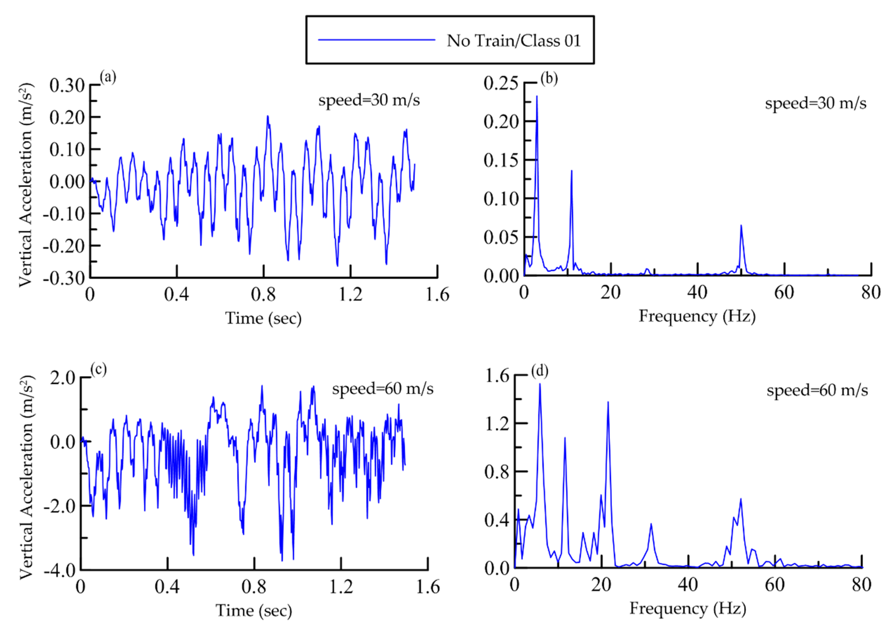
The effect of train speed on the frequency component of ground response is very important to understand. For this reason, time history response and frequency spectrum of the ground acceleration at the center of track for selected cases given in Table 5 are studied. Time history and frequency spectrum of ground acceleration from case 01 (train moving only on the right track) are shown in Figure 10. In case of a train speed of 30 m/s the sharp peaks appear at 2.9 Hz and 11.05 Hz (Figure 10b), which are in close agreement with the results computed using the numerical model proposed by Kouroussis, G., et al. [36]. The given numerical model shows that the peaks at certain frequencies in the ground response spectrum are the function of train geometry (distance between loads or position of wheels) and speed of the train. Similarly, at the train speed of 60 m/s dominant peaks of ground acceleration appear at 5.7 Hz and 22 Hz, as shown in Figure 10d.
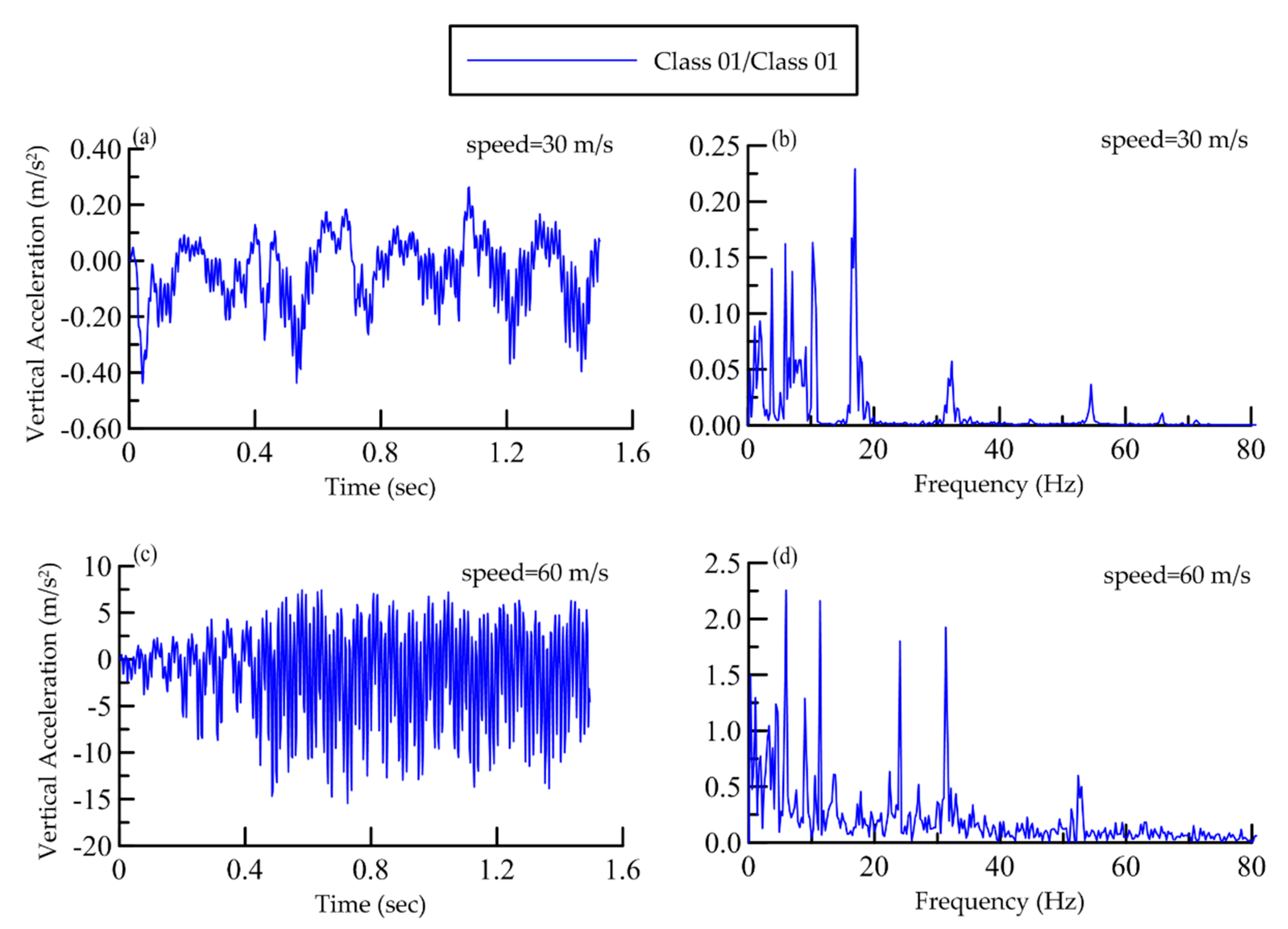
Time history and frequency spectrum of ground acceleration at the center of track from case 02 (trains on both tracks moving in the opposite direction) is shown in Figure 11. It is interesting to note that for the ground response at the train speed of 30 m/s a group of peaks appear near the frequencies that are deemed to be induced from the geometry of train against the train speed. Moreover, at the train speed of 60 m/s not only various peaks at low frequencies but also significant peaks at high frequencies are clearly visible in the frequency spectrum (Figure 11d). A significant increase in the number of peaks at different frequencies in frequency spectrum when trains are traveling on both tracks can be attributed greatly to the fact that vibration radiating from one track due to moving train significantly affect the nearby track.

5. Conclusions

A 3D finite element coupled train–track–soil model is used to predict ground vibration. This study focuses on vibrations radiating from one track and its effect on the nearby track response. At first, the sub-modeling technique is adopted to model the coupled train–track–soil model. The ground, ballasts and sleepers are represented by 3D solid elements and rails on both tracks are modeled by Euler’s beam. The train model and tracks are coupled through dynamic interaction forces between wheels and rails. Finally, a stepwise numerical procedure is used to solve the train–track–soil system. A detailed parametric study is conducted to investigate the influence of track irregularities on the two-way tracks responses at different speeds of the trains. The following conclusions are drawn from the present work.
(1)
When the train is moving on one track, the vibration increase as the train speed increases and the track conditions change from good to worse due to track irregularities.
(2)
The speed of the train has a significant effect on ground vibration. For a given track condition, an increase in speed (when train is moving on one track) causes an increase in ground response as well as shift the response spectra towards high-frequencies e.g., for train speed of 30 m/s the peak appears at 2.9 Hz, whereas it is around 5.7 Hz for 60 m/s.
(3)
The waves propagating due to moving trains on one track have a great influence on a nearby track. When trains are moving on two adjacent tracks the ground vibration induced by each track causes deformation in the tracks. These deformations in the tracks increase the level of track irregularities which consequently cause an increase in impact forces due to the interaction of moving train and track. Based on the results, it is concluded that the response of a track can increase up to 30% when trains are moving on both tracks.
(4)
The tracks have shown significantly different responses when trains are moving on two adjacent tracks. At the speed of 30 m/s a series of low-frequency peaks appear in response spectrum, whereas at speed of 60 m/s the track response spectrum not only exhibits peaks at low frequency but also at high frequency (up to 33 Hz). This significant change in track response is due to the wave propagation from one track to the other track.
(5)
Further studies are needed on the mitigation of track vibration so that a track does not get affected by ground vibration induced by the nearby track.

Author Contributions

D.-H.C. supervised the research and helped in review & editing the manuscript. O.J. conceptualized the idea, performed the numerical simulation and wrote the manuscript. All authors have read and agreed to the published version of the manuscript.

Funding

This research received no external funding.

Conflicts of Interest

The authors declare no conflict of interest.

References

  1. Lefeuve-Mesgouez, G.; Le Houédec, D.; Peplow, A. Ground vibration in the vicinity of a high-speed moving harmonic strip load. J. Sound Vib. 2000, 231, 1289–1309. [Google Scholar] [CrossRef]
  2. Krylov, V.V. Generation of ground vibrations by superfast trains. Appl. Acoust. 1995, 44, 149–164. [Google Scholar] [CrossRef]
  3. Krylov, V.; Ferguson, C. Calculation of low-frequency ground vibrations from railway trains. Appl. Acoust. 1994, 42, 199–213. [Google Scholar] [CrossRef]
  4. Takemiya, H.; Bian, X. Substructure simulation of inhomogeneous track and layered ground dynamic interaction under train passage. J. Eng. Mech. 2005, 131, 699–711. [Google Scholar] [CrossRef]
  5. Kouroussis, G.; Connolly, D.P.; Verlinden, O. Railway-induced ground vibrations—A review of vehicle effects. Int. J. Rail Transp. 2014, 2, 69–110. [Google Scholar] [CrossRef] [Green Version]
  6. Xia, H.; Cao, Y.; De Roeck, G. Theoretical modeling and characteristic analysis of moving-train induced ground vibrations. J. Sound Vib. 2010, 329, 819–832. [Google Scholar] [CrossRef]
  7. Hussein, M.F.M.; Hunt, H.E.M. A numerical model for calculating vibration due to a harmonic moving load on a floating-slab track with discontinuous slabs in an underground railway tunnel. J. Sound Vib. 2009, 321, 363–374. [Google Scholar] [CrossRef]
  8. Ntotsios, E.; Thompson, D.; Hussein, M. The effect of track load correlation on ground-borne vibration from railways. J. Sound Vib. 2017, 402, 142–163. [Google Scholar] [CrossRef]
  9. Yang, W.; Hussein, M.F.M.; Marshall, A.M. Centrifuge and numerical modelling of ground-borne vibration from an underground tunnel. Soil Dyn. Earthq. Eng. 2013, 51, 23–34. [Google Scholar] [CrossRef]
  10. Celebi, E.; Schmid, G. Investigation of ground vibrations induced by moving loads. Eng. Struct. 2005, 27, 1981–1998. [Google Scholar] [CrossRef]
  11. Andersen, L.; Nielsen, S.R.K.; Krenk, S. Numerical methods for analysis of structure and ground vibration from moving loads. Comput. Struct. 2007, 85, 43–58. [Google Scholar] [CrossRef]
  12. Galvín, P.; François, S.; Schevenels, M.; Bongini, E.; Degrande, G.; Lombaert, G. A 2.5D coupled FE-BE model for the prediction of railway induced vibrations. Soil Dyn. Earthq. Eng. 2010, 30, 1500–1512. [Google Scholar] [CrossRef] [Green Version]
  13. Galvín, P.; Romero, A.; Domínguez, J. Fully three-dimensional analysis of high-speed train–track–soil-structure dynamic interaction. J. Sound Vib. 2010, 329, 5147–5163. [Google Scholar] [CrossRef]
  14. Hamarat, M.; Kaewunruen, S.; Papaelias, M.; Silvast, M. New insights from multibody dynamic analyses of a turnout system under impact loads. Appl. Sci. 2019, 9, 4080. [Google Scholar] [CrossRef] [Green Version]
  15. El Kacimi, A.; Woodward, P.K.; Laghrouche, O.; Medero, G. Time domain 3D finite element modelling of train-induced vibration at high speed. Comput. Struct. 2013, 118, 66–73. [Google Scholar] [CrossRef]
  16. Gao, G.; Yao, S.; Yang, J.; Chen, J. Investigating ground vibration induced by moving train loads on unsaturated ground using 2.5D FEM. Soil Dyn. Earthq. Eng. 2019, 124, 72–85. [Google Scholar] [CrossRef]
  17. Gao, G.; Xu, C.; Chen, J.; Song, J. Investigation of ground vibrations induced by trains moving on saturated transversely isotropic ground. Soil Dyn. Earthq. Eng. 2018, 104, 40–44. [Google Scholar] [CrossRef]
  18. Connolly, D.; Giannopoulos, A.; Fan, W.; Woodward, P.K.; Forde, M.C. Optimising low acoustic impedance back-fill material wave barrier dimensions to shield structures from ground borne high speed rail vibrations. Constr. Build. Mater. 2013, 44, 557–564. [Google Scholar] [CrossRef] [Green Version]
  19. Thompson, D.J.; Kouroussis, G.; Ntotsios, E. Modelling, simulation and evaluation of ground vibration caused by rail vehicles. Veh. Syst. Dyn. 2019, 57, 936–983. [Google Scholar] [CrossRef]
  20. Li, T.; Su, Q.; Kaewunruen, S. Saturated ground vibration analysis based on a three-dimensional coupled train-track-soil interaction model. Appl. Sci. 2019, 9, 4991. [Google Scholar] [CrossRef] [Green Version]
  21. Zhou, J.; Chen, X.; Fu, Q.; Xu, G.; Cai, D. Dynamic responses of asphalt concrete waterproofing layer in ballastless track. Appl. Sci. 2019, 9, 375. [Google Scholar] [CrossRef] [Green Version]
  22. Wang, H.; Silvast, M.; Markine, V.; Wiljanen, B. Analysis of the dynamic wheel loads in railway transition zones considering the moisture condition of the ballast and subballast. Appl. Sci. 2017, 7, 1208. [Google Scholar] [CrossRef] [Green Version]
  23. Ribes-Llario, F.; Marzal, S.; Zamorano, C.; Real, J. Numerical modelling of building vibrations due to railway traffic: Analysis of the mitigation capacity of a wave barrier. Shock Vib. 2017, 2017, 11. [Google Scholar] [CrossRef]
  24. Connolly, D.P.; Kouroussis, G.; Laghrouche, O.; Ho, C.L.; Forde, M.C. Benchmarking railway vibrations—Track, vehicle, ground and building effects. Constr. Build. Mater. 2015, 92, 64–81. [Google Scholar] [CrossRef] [Green Version]
  25. Khan, B.L.; Farooq, H.; Usman, M.; Butt, F.; Khan, A.Q.; Hanif, A. Effect of soil–structure interaction on a masonry structure under train-induced vibrations. Proc. Inst. Civil. Eng. Struct. Build. 2019, 172, 922–934. [Google Scholar] [CrossRef]
  26. Zhao, Y.; Shi, Y.; Yang, J. Study of the influence of train vibration loading on adjacent damaged tunnel. Shock Vib. 2019, 2019, 8. [Google Scholar] [CrossRef] [Green Version]
  27. Che, A.; Tang, Z.; Feng, S. An elastic-wave-based full-wavefield imaging method for investigating defects in a high-speed railway under-track structure. Soil Dyn. Earthq. Eng. 2015, 77, 299–308. [Google Scholar] [CrossRef]
  28. Feng, S.J.; Zhang, X.L.; Zheng, Q.T.; Wang, L. Simulation and mitigation analysis of ground vibrations induced by high-speed train with three dimensional FEM. Soil Dyn. Earthq. Eng. 2017, 94, 204–214. [Google Scholar] [CrossRef]
  29. Lysmer, J.; Kuhlemeyer, R.L. Finite dynamic model for infinite media. J. Eng. Mech. Div. 1969, 95, 859–878. [Google Scholar]
  30. Phillips, C.; Hashash, Y.M. Damping formulation for nonlinear 1D site response analyses. Soil Dyn. Earthq. Eng. 2009, 29, 1143–1158. [Google Scholar] [CrossRef]
  31. Bathe, K.-J. Finite Element Procedures; Prentice Hall Inc.: Upper Saddle River, NJ, USA, 1996. [Google Scholar]
  32. Corbin, J. Statistical Representations of Track Geometry: Volume I, Text. 1980; FRA/ORD·Bl/22·2; Federal Railroad Administration: Washington, DC, USA, 1980. [Google Scholar]
  33. Kouroussis, G.; Verlinden, O.; Conti, C. A two-step time simulation of ground vibrations induced by the railway traffic. Proc. Inst. Mech. Eng. Part. C J. Mech. Eng. Sci. 2012, 226, 454–472. [Google Scholar] [CrossRef]
  34. Lei, X.; Noda, N.-A. Analyses of dynamic response of vehicle and track coupling system with random irregularity of track vertical profile. J. Sound Vib. 2002, 258, 147–165. [Google Scholar] [CrossRef]
  35. Ranjan, G.; Rao, A. Basic and Applied Soil Mechanics; New Age International: New Delhi, India, 2007. [Google Scholar]
  36. Kouroussis, G.; Verlinden, O.; Conti, C. Free field vibrations caused by high-speed lines: Measurement and time domain simulation. Soil Dyn. Earthq. Eng. 2011, 31, 692–707. [Google Scholar] [CrossRef]
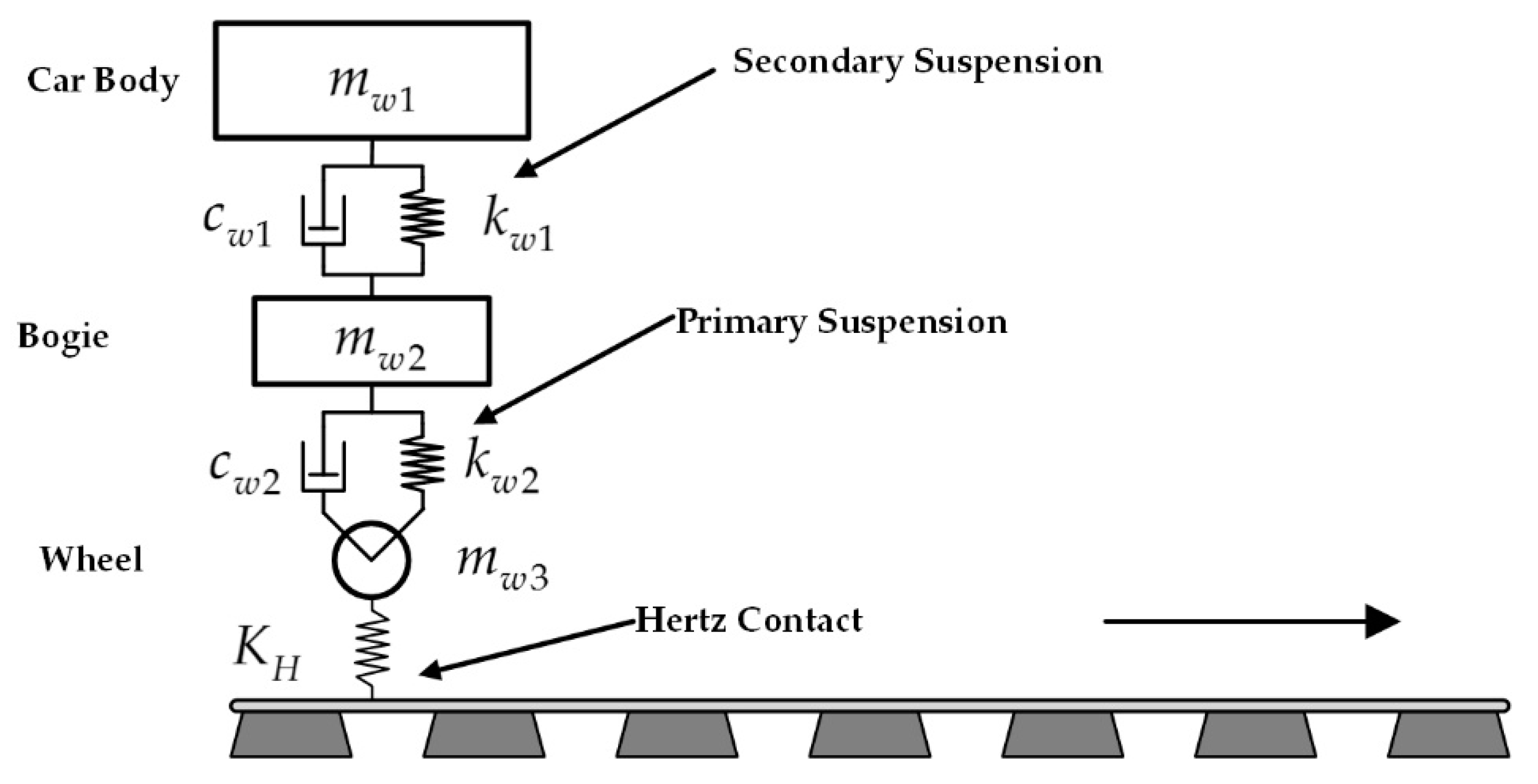
Figure 1. Pictorial representation of the quarter train model.
Applsci 10 00011 g001
Figure 2. Half-space subjected to the point load.
Applsci 10 00011 g002
Figure 3. Comparison of the numerical and analytical solution at the line of observation (0.5 m from surface) (a) longitudinal displacement (b) vertical displacement.
Applsci 10 00011 g003
Figure 4. Configuration of train wheels.
Applsci 10 00011 g004
Figure 5. Profile of the track and ground system: (a) side view, (b) top view, (c) isometric view.
Applsci 10 00011 g005
Figure 6. Vertical track response at the center of tracks at different speeds (Train moving only on right track): (ad) left track, (eh) right track.
Applsci 10 00011 g006
Figure 7. Maximum vertical track response at the center of the track at different speeds (train moving only on right track): (a) left track, (b) right track.
Applsci 10 00011 g007
Figure 8. Vertical track response at the center of the track at different speeds (trains on both tracks moving in the opposite direction): (ad) left track, (eh) right track.
Applsci 10 00011 g008
Figure 9. Maximum Vertical track response at the center of the track at different speeds (trains on both tracks moving in the opposite direction): (a) left track, (b) right track.
Applsci 10 00011 g009
Figure 10. (Left) Time history of ground acceleration at the center of the right track at different speeds (train moving only on right track) (a) speed = 30 m/s (c) speed = 60 m/s, (Right) Frequency spectra of ground acceleration at the center of the right track at different speeds (train moving only on right track) (b) speed = 30 m/s (d) speed = 60 m/s.
Applsci 10 00011 g010
Figure 11. (left) Time history of ground acceleration at the center of right track at different speeds (trains on both tracks moving in opposite direction) (a) speed = 30 m/s (c) speed = 60 m/s, (right) Frequency spectra of ground acceleration at the center of right track at different speeds (trains on both tracks moving in opposite direction) (b) speed = 30 m/s (d) speed = 60 m/s.
Applsci 10 00011 g011
Table 1. Train properties [15].
ParametersValue
Axle load, P (kg)17,679.22
Car mass, m ¯ w 1     (kg)55,963.86
Bogie mass, m ¯ w 2 (kg)3312.313
Wheel mass, m w 3     (kg)1016.047
Hertz contact Stiffness, K H   ( G N / m 1.5 )   93.7
Secondary suspension stiffness,   k w 1     (N/m)1.31 × 10 3  
Primary suspension stiffness, k w 2 (N/m)3.28 × 10 3  
Secondary suspension damping, c w 1 (Ns/m)90
Primary suspension damping, c w 2 (Ns/m)30
Table 2. Rail properties [15].
ParametersValue
Eastic Modulus, E (GPa)210
Density, ρ ( kg / m 3   )7897
Bending stiffness around x, I x ( m 4 )   1.245 × 10⁻⁵
Bending stiffness around z, I z ( m 4 )   4.526 × 10⁻⁶
Torsional stiffness around y, J y ( m 4 )   6.554 × 10⁻³
Table 3. Material properties of sleeper, ballast, and soil [15].
ParametersValue
Sleeper (Concrete)
Elastic Modulus, E (GPa)10
Poisson ratio,0.2
Density, ρ ( kg / m 3   )2400
Primary wave velocity, V p   ( m / s )   2151.6
Secondary wave velocity,   V s   ( m / s )   1317.6
Rayleigh wave velocity,   V r   ( m / s )   1201.2
Ballast
Elastic Modulus, E (GPa)0.13
Poisson ratio,0.4
Density, ρ ( kg / m 3   )1600
Primary wave velocity, V p   ( m / s )   417.3
Secondary wave velocity,   V s   ( m / s )   170.3
Rayleigh wave velocity,   V r   ( m / s )   160.3
Soil
Elastic Modulus, E (GPa)0.025
Poisson ratio,0.45
Density, ρ ( kg / m 3   )1800
Primary wave velocity, V p   ( m / s )   229.5
Secondary wave velocity,   V s   ( m / s )   69.2
Rayleigh wave velocity,   V r   ( m / s )   65.6
Table 4. Track classes and parameters [33].
ParametersTrack Classes
654321
A ( × 10 6   m )     0.09540.16750.29680.53000.95401.6748
  ϕ 1 ( × 10 3   m 1 )   23.9423.9423.9423.9423.9423.94
  ϕ 2 ( × 10 2 m 1   )13.12313.12313.12313.12313.12313.123
Table 5. Train and tracks condition on the left and right track.
Case 01 (Left Track/Right Track)
Train Moving Only on Right Track
Case 02 (Left Track/Right Track)
Trains Moving on Both Tracks But Opposite in Direction
no train/no irregularitiesno irregularities/no irregularities
no train/class 01class 01/no irregularities
no train/class 02class 02/no irregularities
no train/class 03class 03/no irregularities
no train/class 04class 04/no irregularities
no train/class 05class 05/no irregularities
no train/class 06class 06/no irregularities
\class 01/class 01
\class 02/class 01
\class 03/class 01
\class 04/class 01
\class 05/class 01
\class 06/class 01
\class 02/class 02
\class 03/class 02
\class 04/class 02
\class 05/class 02
\class 06/class 02
\class 03/class 03
\class 04/class 03
\class 05/class 03
\class 06/class 03
\class 04/class 04
\class 05/class 04
\class 06/class 04
\class 05/class 05
\class 06/class 05
\class 06/class 06