Abstract
Simulating shallow water flows in large scale river-lake systems is important but challenging because huge computer resources and time are needed. This paper aimed to propose a simple and efficient 1D–2D coupled model for simulating these flows. The newly developed lattice Boltzmann (LB) method was adopted to simulate 1D and 2D flows, because of its easy implementation, intrinsic parallelism, and high accuracy. The coupling strategy of the 1D–2D interfaces was implemented at the mesoscopic level, in which the unknown distribution functions at the coupling interfaces were calculated by the known distribution functions and the primitive variables from the adjacent 1D and 2D lattice nodes. To verify the numerical accuracy and stability, numerical tests, including dam-break flow and surge waves in the tailrace canal of a hydropower station, were simulated by the proposed model. The results agreed well with both analytical solutions and commercial software results, and second-order convergence was verified. The application of the proposed model in simulating the surge wave propagation and reflection phenomena in a reservoir of a run-of-river hydropower station indicated that it had a huge advantage in simulating flows in large-scale river-lake systems.
1. Introduction
One-dimensional (1D) and two-dimensional (2D) shallow water equations are widely used to simulate flows in rivers, lakes, reservoirs, and estuaries. The dimensionally different models are suitable for different scenarios. The cross-sectional integrated 1D models are extremely suitable for hydrodynamic simulations in large scale river networks, with their lumped boundary representations for hydraulic structures, such as weirs, dams, culverts, and pumps. On the other hand, 2D models, with their ability to accurately resolve flows in both longitudinal and transversal directions, are the primary choice for hydrodynamic simulations for lakes, reservoirs, and estuaries. Because 1D river networks and 2D lakes are often linked together, it is natural to choose the 1D-2D coupled model for accurately investigating their interactions.
The numerical solvers for the shallow water equations are mainly based on traditional methods, such as an implicit finite-difference scheme for the 1D model and finite-volume method for the 2D model [1,2,3]. Even if being accepted widely, these traditional methods are relatively difficult to implement, and the calculations are usually time-consuming. Recently, the lattice Boltzmann (LB) method is developed for simulating complicated fluid flow problems, such as multi-dimensional hydrodynamic flows [4,5], multiphase flows [6,7], porous media flows, and fluid-structure interaction problems [8]. Its easy implementation, intrinsic parallelism, and high accuracy have been demonstrated by many works [5,8,9]. Because of these advantages, introducing the LB method into simulations of the shallow water flows seems to be very attractive. Cheng [10,11] first introduced a 1D LB model for the 1D shallow-water equations, and Frandsen [12] had further verified the model. Later, Thang [13] used it to simulate flows in complex irrigation channels, and Chopard [14] used it to simulate flows in rapids canals. On the other hand, Zhou [15] first developed a 2D LB model for the shallow water equations, in which the terrain and riverbed friction were represented by source terms in the original LB equation. Cheng and Zhang [4,9,16] used a similar 2D LB model to simulate the surge propagations caused by the transient processes of hydropower stations. Liu [17,18,19] adopted the 2D models to simulate flows in open channels and shallow lakes.
This paper aimed to propose a 1D–2D coupled model for simulating shallow water flows in river-lake systems. Thus, it is necessary to discuss the 1D–2D coupling strategies. According to the specific problems, the strategies are mainly divided into three categories: the lateral coupling, the superposition coupling, and the boundary connected coupling [20]. The first category is mainly adopted to simulate flows in floodplain systems [2,21,22]. The second category is mainly used to simulate flows in systems with obvious 2D flow effects of local flow patterns, in which the high-dimensional model is superimposed on the low-dimensional global model [23,24]. The third category is mainly applied to rivers, lakes, reservoirs, and estuarine systems, which connect different dimensional models directly through the coupling boundaries. There are a variety of coupling strategies available for the third category. The simplest one is to run each submodel in sequence, with its boundary conditions provided by the previous solution of each other [25,26]. However, the mutually provided boundary conditions are lagged, causing the non-conservation of mass or momentum. To reduce the errors, overlapped areas are set at the coupling boundaries [27,28,29], but it still cannot avoid the errors caused by the lagged boundary conditions. Another strategy is to use iterative methods to solve the coupling boundaries, which can fully meet the conservation of mass and momentum [20,30]. However, each iteration must go through an overall calculation, and one time step may need several iterations, resulting in a great calculation amount and a low computational efficiency.
The coupling strategies listed above are tailored for traditional numerical methods. But for the LB method, the coupling strategy can be implemented at the mesoscopic level since it solves hyperbolic equations at the mesoscopic level. Currently, the works addressing the coupling procedure of interconnected subdomains for the LB-based shallow water simulations are rare. We found only one similar work that tried to couple a 2D shallow water submodel with 2D free-surface submodel [29], but the coupling strategy was still implemented at the macroscopic level, and the numerical stability was affected by both relaxation time and the size of the overlapping region.
Here, we presented a rather simple and efficient 1D–2D coupled shallow water model, with the coupling strategy at the mesoscopic level. The coupling interface was regarded as an interior lattice node of the 1D domain with only three unknown distribution functions to be solved, and the numerical stability was only affected by the relaxation time. Moreover, the proposed model retained all the merits of the LB method [31,32], especially its intrinsic parallelism, convenient processing complex boundaries, and easy programming, making it quite suitable for hydrodynamic simulations on a large scale river-lake systems.
The paper is organized as follows. The 1D–2D coupled model is described in Section 2. Numerical tests are carried out to verify the accuracy and stability of the proposed model in Section 3. An application to simulating the surge wave propagation and reflection processes in a practical run-of-river hydropower station is presented in Section 4. Finally, a brief conclusion is made to end the article.
2. 1D and 2D Shallow Water Submodels and Their Coupling Strategy
2.1. 1D Shallow Water Submodel
The 1D shallow-water equations can be expressed as
where h is the water depth, u is the velocity, x is the spatial coordinate, t is the temporal coordinate, g is the gravitational acceleration, z is the water surface elevation. is the frictional loss, in which n is the Manning roughness coefficient, and R is the hydraulic radius.
The LB method has been used to numerically solve the 1D flows governed by the Equations (1) and (2). The D1Q3 model geometry has been chosen, in which , and . The common LB equation [10] with Bhatnagar–Gross–Krook (BGK) collision operator can be written as
where the left side terms of Equation (3) denote the propagation process, and the right side terms of Equation (3) denote the collision process. x is the lattice node coordinate, is the discrete particle velocity, is the discrete distribution function along the particle velocity direction, is its corresponding equilibrium, is the relaxation time, and is the external forcing term.
The equilibrium distribution functions can be expressed as
Water depth and velocity of the fluid are defined as
The Chapman–Enskog expansion [10] can be adopted to recover the physics of the 1D shallow-water Equations (1) and (2). The viscosity and relaxation time must satisfy the following relation.
The treatment of external forcing term proposed by Cheng [10] has been adopted, and can be written as
As for boundary treatment, the unknown distribution functions at the inlet and outlet boundary can be defined as
2.2. 2D Shallow Water Submodel
The 2D shallow-water equations can be expressed as
where ui and uj are the depth-averaged velocities; , with as the hydraulic gradient caused by the bed gradient, is the bed elevation; is the hydraulic gradient caused by bed shear stresses, in which n is Manning roughness coefficient.
The LB method has been used to numerically solve the 2D flows governed by the Equations (10) and (11). The lattice Boltzmann equation [31] can be expressed as
where is the collision operator; the definition of other variables are the same as Equation (3).
The D2Q9 model has been applied, and the discrete particle velocities are
The equilibrium distribution functions are expressed as
where the weight factor .
Water depth and velocity of the fluid are given by Equation (5).
The multi-relaxation time (MRT) collision operator has been adopted [33]. The particle distribution functions are transformed into moment spaces before the relaxation step: , where M denotes the transformation matrix from the distribution functions to the moments, and the diagonal collision matrix contains the relaxation parameters. The relaxation parameters except are within the range [0, 2], and the optimal values for these parameters depend on the specific geometry, the initial conditions, and boundary conditions of the system. In this study, , is related to the kinematic viscosity , which is defined as
With the above setups, the 2D LB submodel can recover 2D shallow-water Equations (10) and (11) by the Chapman–Enskog expansion in the incompressible flow [34].
Second-order treatment of the external forcing term proposed by Cheng [35] has been adopted. Assuming the A is the source term in the continuity Equation (10) and is the external forcing term in the momentum Equation (11), the can be written as
in which , , with g regarded as a vector in .
2.3. The Coupling Strategy of 1D and 2D Submodels
The coupling strategy of the 1D–2D interfaces is implemented at the mesoscopic level, in which the distribution functions are used to couple 1D and 2D submodels. The coupling interface is in the form of a node in the 1D computational domain, and in the form of a line in the 2D computational domain. In this study, the coupling interface was treated as an interior lattice node of the 1D domain, with three unknown distribution functions to be calculated. These unknown distribution functions at the coupling interface were calculated by the distribution functions and macroscopic variables from the adjacent 1D and 2D lattice nodes. The reformulation of the unknown distribution function is depicted in Figure 1, in which denote distribution functions of the 1D domain, denote distribution functions of the 2D domain, k refers to the position of the coupling node at the 1D domain, j refers to time, and m denotes the position of the coupling node at the 2D domain.
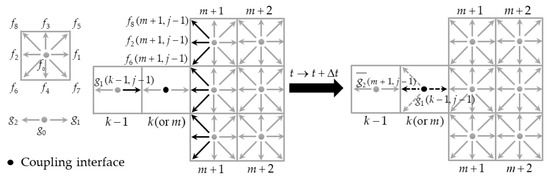
Figure 1.
Sketch of the 1D–2D coupling boundary.
The processing steps for dealing coupling interface can be expressed as follows:
- (1)
- Calculate the three unknown distribution functions of the coupling interface;
- (2)
- Calculate the macroscopic parameters (water depth and velocity) of the coupling interface by the distribution functions solved in the first step;
- (3)
- Calculate the unknown distribution functions at the coupling boundaries of the 2D domain by the above calculated macroscopic parameters.
To be specific, the unknown distribution functions , , of the coupling interface are calculated at first. can be expressed as
can be calculated by the distribution functions at the adjacent 2D nodes and expressed as
where , with , , and as the averaged values of distribution functions at position m + 1.
can be calculated by
Then, the water depth and velocity at the coupling interface can be obtained by
Finally, the unknown distribution functions of lattice nodes at the inlet boundary of the 2D domain can be disposed of as following [36]: given , , , assuming that . The unknown distribution functions , , and at the inlet boundary of the 2D domain can be calculated by Equation (23).
Similarly, the unknown distribution functions , , and at the outlet boundary of the 2D domain can be solved by Equation (24). Other boundaries of the 2D domain are regarded as no-slip wall boundary conditions and treated by a non-equilibrium extrapolation scheme [37].
The above coupling strategy is aimed at the condition that the 1D domain is at the upstream, and the 2D domain is at the downstream, with the coupling interface at the inlet boundary of the 2D domain. In the reverse condition, the coupling interface is at the outlet boundary of the 2D domain. The unknown distribution functions and macroscopic parameters of the interface are solved in the same way as the above condition.
2.4. Stability Requirements
The LB method for shallow water flows must satisfy the stability requirements, which can be expressed as
where Cn is Courant number, and Fr is Froude number.
3. Numerical Experiments
To evaluate the accuracy and stability of the 1D–2D coupled model, the dam break flow and the surge wave flow in the tailrace canal of a hydropower station were simulated. The 1D–2D coupled model could be implemented on the graphic processing unit (GPU) or central processing unit (CPU) platform. In this study, all cases were executed on a GPU platform, and the specific GPU implementation could be found in [16].
3.1. The Dam Break Flow
The dam break flow in a frictionless and flat rectangular channel was simulated, and its analytic solutions are given by Stoker [38]. As shown in Figure 2, the dam was placed across the channel at the middle plane of the domain, and the initial water depths at the upstream and downstream sides were set to 8 m and 2 m, respectively. In simulations, the channel was divided into three domains, with the middle domain simulated by the 2D submodel, and the two outer domains simulated by the 1D submodel. The upstream and downstream boundaries were set to constant water depths. The lateral boundaries of the 2D domain were treated as no-slip wall boundary conditions. x1 and x2 were the coupling interfaces, which were located at the inlet and outlet boundaries of the 2D domain, respectively. The initial velocity was zero. When the dam collapsed completely in a sudden, two bores propagating in the upstream and downstream directions, respectively, were generated.
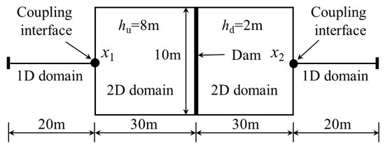
Figure 2.
Computational domain of the dam break case.
In simulations, unless mentioned otherwise, the values of the relaxation parameters for the 1D and 2D submodels were taken to be and , respectively. We verified the accuracy and stability of the 1D–2D coupled model by analyzing its grid convergence, errors, and convergence rate.
Firstly, the grid convergence of the 1D–2D coupled model was analyzed, and the lattice spacing ranged from 0.05 m to 0.4 m, with each one doubled from the former. As shown in Figure 3, the numerical results approached the analytic solution as the mesh became finer. But as the mesh became very fine, such as lattice spacing 0.05 m and 0.1 m, the result differences between them were very small. To get an accurate solution and to improve the computational efficiency, the lattice spacing of 0.1 m was reasonable, which was adopted in the following simulation.
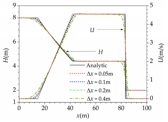
Figure 3.
Water depth and velocity profiles of the 1D–2D coupled model at t = 4 s under different lattice spacing.
Then, the accuracy of the proposed model was analyzed by comparing its results with those of the 1D model, 2D model, and analytic solution. Note that the results of the 2D part were the average values in the y-direction. In Figure 4, water depth and velocity profiles of the three numerical models almost coincided with each other and agreed well with the analytic solutions.
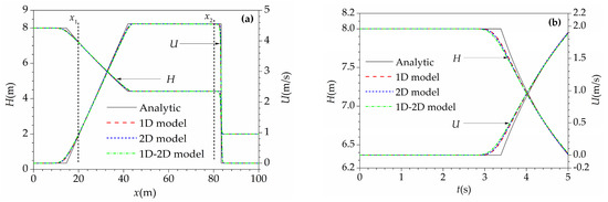
Figure 4.
Water depth and velocity profiles of different models for the dam break flow (, , , Fr 0.691): (a) water depth and velocity profiles at t = 4 s, and (b) water depth and velocity histories at coupling interface x1.
Table 1 shows the errors of three numerical models at x1 and x2, respectively. The errors of the proposed model were closed to those of the 2D model and slightly larger than those of the 1D model, but still quite small. The absolute errors for water depth were within 0.04 m, and the relative errors were within 0.5%. The errors for velocity was a little larger, with a maximum absolute error of 0.045 m/s, and the corresponding relative error of 4.97%, which is acceptable in practical engineering.

Table 1.
At coupling interfaces of the three models at t = 4 s (absolute error (AE), relative error (RE)).
Finally, the accuracy of the 1D–2D coupled model was studied by measuring the convergence rate of the relative global error as the lattice spacing changes, where the relative global error is defined as
where u is the numerical solution, ua is the analytic solution.
The relaxation parameters of 1D and 2D submodels calculated by Equations (6) and (15), respectively, were divided into three cases: (1) and , (2) and , and (3) and . For each case, four lattice spacing 0.05 m, 0.1 m, 0.2 m, and 0.4 m were tested. In Figure 5, the relative global errors were plotted natural logarithmically as functions of the lattice spacing. The slopes of the least-squares fits were 1.92, 1.916, and 1.901 for the above three cases, respectively, indicating the second-order accuracy of the 1D–2D coupled model for the dam break flow.
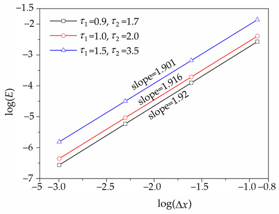
Figure 5.
Convergence rate of the 1D–2D coupled model for the dam break flow.
3.2. The Surge Waves in Tailrace Canal of a Hydropower Station
The surge waves in the tailrace canal of a hydropower station caused by load rejection were simulated by the 1D–2D coupled model. The tailrace canal had a constant rectangular cross-section with a length of 100 m, a width of 10 m, a flat bottom, and a Manning roughness coefficient of 0.015. The upstream boundary was a given discharge, which decreased linearly from 600 m3/s to 0 m3/s within 8 s. The downstream boundary was a constant water depth of 15 m. The lateral boundaries of the 2D domain were treated as no-slip wall boundary conditions. As depicted in Figure 6, the 2D submodel and 1D submodel were used to simulate the upstream half part and downstream half part of the domain, respectively. The interface was at x = 50 m, which was also at the outer boundary of the 2D domain. The lattice spacing was 0.2 m, the time step was 0.01 s, and the relaxation parameters were and .
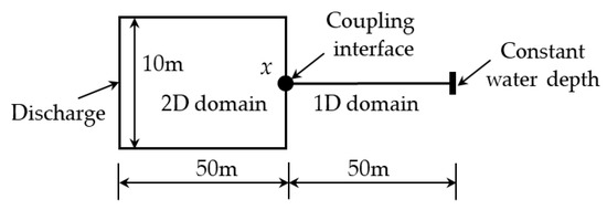
Figure 6.
Computational domain for the surge waves in the tailrace canal of a hydropower station.
The discharge and water depth histories of the 1D–2D coupled model and commercial software Delft3D were compared in Figure 7. The results agreed well with each other, and the proposed method had a better ability to capture the steep inflection point of the surge, indicating a smaller numerical diffusivity.
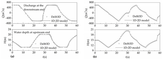
Figure 7.
Surge wave histories in the tailrace canal for load rejection: (a) water depth at the upstream end and discharge at the downstream end; (b) water depth and discharge histories at the coupling interface (x = 50 m).
4. Simulation of Surge Waves in the Reservoir of a Run-of-River Hydropower Station
4.1. Computational Setup
The surge wave propagation and reflection phenomena caused by a load rejection in a run-of-river hydropower station were simulated to further demonstrate the capability of the proposed 1D–2D coupled model. The hydropower station, the reservoir, and the computational domain are depicted in Figure 8. The reservoir was divided into three parts (Channel 1 (C1), Channel 2 (C2), and channel 3 (C3)) by two dikes (Dike 1 (D1) and Dike 2 (D2)). Two powerhouses—Powerhouse 1 (PH1) and Powerhouse 2 (PH2)—were located at the end of Channel 2. Powerhouse 1 included 14 turbines, with a total discharge of 11550 m3/s, and Powerhouse 2 included seven turbines, with a total discharge of 6385 m3/s. Channel 1 and Channel 3 were used for sand washing and shipping. There were two side branches: Branch 1 was 7.7 km, and Branch 2 was 2.2 km. Several monitoring points were set to record the flow parameters. Point A was located at the inlet of Powerhouse 1, Point B was located at the inlet of Powerhouse 2, Point C was located at the head of Dike 1, Point D was located at the head of Dike 2, Point E was located at the estuary of Branch 1, Point F was located at the estuary of Branch 2, and Point G was located at the coupling interface.
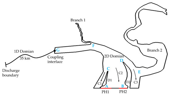
Figure 8.
Schematic of the reservoir region of the computational domain.
The simulation scope of this example was about 40 km, in which the 2D part of the reservoir (about 5 km starting from the dam to Point G) was treated by the 2D submodel, and the upstream 35 km river was handled by the 1D submodel. The upstream boundary of the 1D domain was set to constant discharge. The downstream boundary of the 2D domain was the dam, at which the discharge values of each powerhouse were given. Other boundaries of the 2D domain were set to no-slip wall boundary conditions. The Manning roughness coefficient of the river bed was 0.025. The time steps of 1D and 2D submodels were both set to 0.0864 s, and the corresponding uniform lattice length was 4.32 m. The mesh nodes were 8102 for the 1D domain and 1600 1200 for the 2D domain.
4.2. Simulation Results
The steady flow simulation was conducted at first, and its results were used as the initial conditions for the transient simulation. The transient process simulation was caused by the load rejection of all units in two powerhouses simultaneously, and the discharge decreased linearly to zero within 40 s. The water depth and velocity at six typical moments are shown in Figure 9.
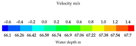
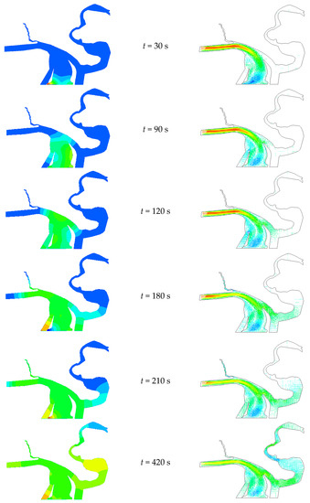
Figure 9.
Surge wave propagation and reflection in the reservoir after load rejection: water depth (left column) and velocity (right column).
After the load rejection, a pair of surge waves generated from two powerhouses and propagated upstream (t = 30 s). Then, the surge wave propagated back and forth between Dike 1 and Dike 2, causing the water depths near two dikes to fluctuate alternately. This phenomenon was particularly obvious in the preliminary stages of the transient simulation (t = 90 s and t = 120 s). At about t = 120 s, the surge waves reached the estuary of Branch 1 and Branch 2 for the first time, respectively. Meanwhile, it also reached the front of Channel 1, which caused an obvious increase in water depth (t = 120 s and t = 180 s). The surge wave kept propagating; at about t = 210 s, it reached the coupling interface. At about t = 420 s, it arrived at the end of Branch 1.
To analyze the fluctuation of water depth at each important building of the hydraulic project, Figure 10 shows the histories of water depth at some monitoring points. Many information could be extracted from the monitoring data, such as the first moment affected by the surge waves, the maximum and the minimum water depths, and the attenuation duration of the surge waves. Take point A, for example, the maximum and the minimum water depths were 68.77 m and 67.49 m, which occurred around 0.85 and 2 h, respectively. The time for the surge wave to attenuate completely was about 5 h.
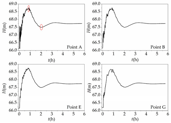
Figure 10.
Water depth histories of some monitoring points.
To study the propagation and reflection rules of the surge waves, we enlarged the histories of water depth at the inlet of the two powerhouses. As shown in Figure 11, the surge waves were composed of the low-frequency fundamental wave and high-frequency wave. The former was caused by the propagation and reflection of surge waves between two powerhouses and upstream boundaries, and the latter was caused by the propagation and reflection of surge waves between dikes and banks. The riverbed resistance attenuated these fluctuations gradually during the propagation process, which took about 1 h and 5 h to calm down the high-frequency wave and the low-frequency fundamental wave, respectively.
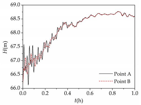
Figure 11.
Comparison of water depth at the inlets of Powerhouse 1 and Powerhouse 2.
4.3. Computational Efficiency Analysis
The GPU card equipped with a large number of computing units and massive thread parallelism has shown powerful capability in non-graphical computations. The LB method has explicit and local features, which match the multi-thread parallel characteristics of GPU quite well. Thus, the 1D–2D coupled model could fully take advantage of the GPU to solve the computational intensive problem. The 1D–2D coupled model was implemented on a GPU platform, and the specific GPU implementation of the LB method could be found in [17]. All computations were carried out using double precision floating on an NVIDIA Geforce GTX TITAN X graphics card, which could deliver a peak performance of approximately 7 × 10¹² single-precision floating-point operations per second and a peak memory bandwidth of approximately 336.5 GB/s.
To verify the strong ability of the 1D–2D coupled model in computational intensive problem, we compared the computational efficiencies of the proposed model in different mesh sizes. Four different lattice spacing 2.16 m, 4.32 m, 8.64 m, and 17.28 m were selected. As shown in Table 2, the consumed time referred to the computational time, given in hours, and the performance denoted the updated number of nodes per second, given in Millions of Node Updates Per Second (MNUPS). The speedup ratio represented the ratio of the computational performance of other mesh sizes to that of the coarsest mesh ( = 17.28). As we could see that as the mesh became finer, the consumed time increased, but the performance and the speedup ratio increased, indicating that the proposed model could achieve better performances on finer meshes. Therefore, the 1D–2D coupled model had an outstanding advantage in simulating flows in large-scale river-lake systems.
Table 2.
Performance of the 1D–2D coupled model under different mesh sizes.
5. Conclusions
In this work, a 1D–2D coupled model was developed for shallow water simulations in large scale river-lake systems, in which both 1D and 2D submodels were numerically solved by the LB method. Unlike any other existing coupling approaches, the coupling strategy of the proposed model was carried out at the mesoscopic level. The distribution functions of the LB equation replaced the role of water depth and discharged to bridge the 1D and 2D submodels. The coupling interface was treated as an interior lattice node of the 1D domain, and its unknown distribution functions were calculated by the macroscopic variables and the distribution functions from the adjacent 1D and 2D lattice nodes. The proposed approach was rather simple and of high efficiency because there was no iterative process.
Numerical tests on two benchmark cases showed that the numerical solutions using the proposed model were in excellent agreement with the analytical solutions and commercial software results, and second-order convergence was observed, indicating the proposed model had good accuracy. The application in simulating the surge wave propagation and reflection phenomena in the reservoir of a run-of-river hydropower station had shown that the proposed model could achieve better performances on finer meshes, indicating its high computational efficiency in the computational intensive problem. Therefore, the 1D–2D coupled model had a huge potential to simulate flows in large-scale river-lake systems.
The proposed model retained all the merits of the LB method, which were simple, high accuracy, convenient processing complex boundaries, suitable for parallel computing, and wide application range. Thus, it has great value for applications. Further studies of the 1D–2D coupled model would focus on its applications on simulations of water temperature, water quality, and sediment transport in large scale river-lake systems.
Author Contributions
Conceptualization, W.M. and Y.C.; methodology, W.M. and J.W.; software, W.M. and J.W.; validation, W.M.; writing—original draft, W.M. and C.Z.; writing—review and editing, W.M., Y.C., C.Z. and L.X. All authors have read and agreed to the published version of the manuscript.
Funding
This research was funded by the National Natural Science Foundation of China (NSFC) (Grant No. 51839008 and 51579187), and Natural Science Foundation Project of CQ CSTC (Grant No. KJQN201800712).
Acknowledgments
Our grateful thanks to Zhiyan Yang for his valuable advice for revising the manuscript.
Conflicts of Interest
The authors declare no conflict of interest.
References
- Adeogun, A.G.; Daramola, M.O.; Pathirana, A. Coupled 1D-2D hydrodynamic inundation model for sewer overflow: Influence of modeling parameters. Water Sci. 2015, 29, 146–155. [Google Scholar] [CrossRef]
- Liu, Q.; Qin, Y.; Zhang, Y.; Li, Z. A coupled 1D-2D hydrodynamic model for flood simulation in flood detention basin. Nat. Hazards 2015, 75, 1303–1325. [Google Scholar] [CrossRef]
- Morales-Hernández, M.; García-Navarro, P.; Burguete, J.; Brufau, P. A conservative strategy to couple 1D and 2D models for shallow water flow simulation. Comput. Fluids 2013, 81, 26–44. [Google Scholar] [CrossRef]
- Zhang, C.; Cheng, Y.; Wu, J.; Diao, W. Lattice Boltzmann simulation of the open channel flow connecting two cascaded hydropower stations. J. Hydrodyn. 2016, 28, 400–410. [Google Scholar] [CrossRef]
- Peng, Y.; Diao, W.; Zhang, X.; Zhang, C.; Yang, S. Three-Dimensional Numerical Method for Simulating Large-Scale Free Water Surface by Massive Parallel Computing on a GPU. Water 2019, 11, 2121. [Google Scholar] [CrossRef]
- Fakhari, A.; Geier, M.; Lee, T. A mass-conserving lattice Boltzmann method with dynamic grid refinement for immiscible two-phase flows. J. Comput. Phys. 2016, 315, 434–457. [Google Scholar] [CrossRef]
- Cai, L.; Xu, W.; Luo, X. A Double-Distribution-Function Lattice Boltzmann Method for Bed-Load Sediment Transport. Int. J. Appl. Mech. 2017, 9, 1750013. [Google Scholar] [CrossRef]
- Wu, J.; Cheng, Y.; Zhou, W.; Zhang, C.; Diao, W. GPU acceleration of FSI simulations by the immersed boundary-lattice Boltzmann coupling scheme. Comput. Math. Appl. 2016, 78, 1194–1205. [Google Scholar] [CrossRef]
- Zhang, C.; Cheng, Y.; Li, Y. Lattice Boltzmann model for two-dimensional shallow water flows realizing parallel computing on GPU. J. Hydrodyn. 2011, 26, 194–200. [Google Scholar]
- Cheng, Y. Application of the lattice boltzmann method-one dimensional dam breaker simulation. Mech. Eng. 2000, 22, 47–48. [Google Scholar]
- Cheng, Y.; Suo, L. A lattice BGK lodel for simulating one-Dimensional unsteady open channel flows. Adv. Water Sci. 2000, 11, 362–367. [Google Scholar]
- Frandsen, J.B. A simple LBE wave runup model. Prog. Comput. Fluid Dyn. Int. J. 2008, 8, 222. [Google Scholar] [CrossRef]
- Van Thang, P.; Chopard, B.; Lefèvre, L.; Ondo, D.A.; Mendes, E. Study of the 1D lattice Boltzmann shallow water equation and its coupling to build a canal network. J. Comput. Phys. 2010, 229, 7373–7400. [Google Scholar] [CrossRef]
- Chopard, B.; Pham, V.T.; Lefèvre, L. Asymmetric lattice Boltzmann model for shallow water flows. Comput. Fluids 2013, 88, 225–231. [Google Scholar] [CrossRef]
- Zhou, J.G. A lattice Boltzmann model for the shallow water equations. Comput. Methods Appl. Mech. Engrg. 2002, 191, 3527–3539. [Google Scholar] [CrossRef]
- Cheng, Y.; Suo, L. 2D open channel flow simulations by the lattice Boltzmann model. Adv. Water Sci. 2003, 14, 9–14. [Google Scholar]
- Liu, H.; Zhou, G.J.; Burrows, R. Lattice Boltzmann model for shallow water flows in curved and meandering channels. Int. J. Comut. Fluid Dyn. 2009, 23, 209–220. [Google Scholar] [CrossRef]
- Liu, H.; Zhu, Z.; Liu, J.; Liu, Q. Numerical analysis of the impact factors on the flow fields in a large shallow lake. Water 2019, 11, 155. [Google Scholar] [CrossRef]
- Liu, H.; Ding, Y.; Wang, H.; Zhang, J. Lattice Boltzmann method for the age concentration equation in shallow water. J. Comput. Phys. 2015, 299, 613–629. [Google Scholar] [CrossRef]
- Chen, Y.; Wang, Z.; Liu, Z.; Zhu, D. 1D–2D Coupled Numerical Model for Shallow-Water Flows. J. Hydraul. Eng. 2011, 138, 122–132. [Google Scholar] [CrossRef]
- Kuiry, S.; Sen, D.; Bates, P.D.; Yan, D. Application of the 1D-quasi 2D model tinflood for floodplain inundation prediction of the river thames. ISH J. Hydraul. Eng. 2011, 17, 98–110. [Google Scholar] [CrossRef]
- Prestininzi, P.; Di Baldassarre, G.; Schumann, G.; Bates, P.D. Selecting the appropriate hydraulic model structure using low-resolution satellite imagery. Adv. Water Resour. 2011, 34, 38–46. [Google Scholar] [CrossRef]
- Marin, J.; Monnier, J. Superposition of local zoom models and simultaneous calibration for 1D-2D shallow water flows. Math. Comput. Simul. 2009, 80, 547–560. [Google Scholar] [CrossRef]
- Fernández-Nieto, E.D.; Marin, J.; Monnier, J. Coupling superposed 1D and 2D shallow-water models: Source terms in finite volume schemes. Comput. Fluids 2010, 39, 1070–1082. [Google Scholar] [CrossRef]
- Steinebach, G.; Rademacher, S.; Rentrop, P.; Schulz, M. Mechanisms of coupling in river flow simulation systems. J. Comput. Appl. Math. 2004, 168, 459–470. [Google Scholar] [CrossRef][Green Version]
- Twigt, D.J.; De-Goede, E.D.; Zijl, F.; Schwanenberg, D.; Chiu, A.Y.W. Coupled 1D-3D hydrodynamic modelling, with application to the Pearl River Delta. Ocean. Dyn. 2009, 59, 1077–1093. [Google Scholar] [CrossRef]
- Zhang, X.X.; Cheng, Y.G.; Yang, J.D.; Xia, L.S.; Lai, X. Simulation of the load rejection transient process of a francis turbine by using a 1D-3D coupling approach. J. Hydrodyn. 2014, 26, 715–724. [Google Scholar] [CrossRef]
- Bladé, E.; Gómez-Valentín, M.; Dolz, J.; Aragón-Hernández, J.L.; Corestein, G.; Sánchez-Juny, M. Integration of 1D and 2D finite volume schemes for computations of water flow in natural channels. Adv. Water Resour. 2012, 42, 17–29. [Google Scholar] [CrossRef]
- Thorimbert, Y.; Lätt, J.; Chopard, B. Coupling of lattice Boltzmann shallow water model with lattice Boltzmann free-surface model. J. Comput. Sci. 2019, 33, 1–10. [Google Scholar] [CrossRef]
- Yu, K.; Chen, Y.; Zhu, D.; Variano, E.A.; Lin, J. Development and performance of a 1D–2D coupled shallow water model for large river and lake networks. J. Hydraul. Res. 2018, 57, 1–14. [Google Scholar] [CrossRef]
- Guo, Z.; Zheng, C. Theory and Applications of Lattice Boltzmann Method; Science Press: Beijing, China, 2009; ISBN 9787030235893. [Google Scholar]
- He, Y.; Wang, Y.; Li, Q. lattice Boltzmann Method: Theory and Application; Science Press: Beijing, China, 2009; ISBN 9787030232724. [Google Scholar]
- Ginzburg, I. Multiple-relaxation-time lattice Boltzmann. R. Soc. 2002, 360, 437–451. [Google Scholar]
- Chen, H.; Chen, S.; Matthaeus, W.H. Recovery of the Navier-Stokes equations using a lattice-gas Boltzmann method. Phys. Rev. A 1992, 45, 5339–5342. [Google Scholar] [CrossRef] [PubMed]
- Cheng, Y.; Li, J. Introducing unsteady non-uniform source terms into the lattice Boltzmann model. Int. J. Numer. Methods Fluids 2008, 56, 629–641. [Google Scholar] [CrossRef]
- Zou, Q.; He, X. On pressure and velocity flow boundary conditions and bounceback for the lattice Boltzmann BGK model. Phys. Fluids 1997, 9, 1591–1598. [Google Scholar] [CrossRef]
- Guo, Z.; Zheng, C.; Shi, B. Non-equilibrium extrapolation method for velocity and pressure boundary conditions in the lattice boltzmann method. Chin. Phys. 2002, 11, 366–374. [Google Scholar]
- Stoker, J.J. Water Waves; Pure and Applied Mathematics; Interscience Publisher: Geneva, Switzerland, 1957. [Google Scholar]
© 2019 by the authors. Licensee MDPI, Basel, Switzerland. This article is an open access article distributed under the terms and conditions of the Creative Commons Attribution (CC BY) license (http://creativecommons.org/licenses/by/4.0/).