Estimating Conditional Value at Risk in the Tehran Stock Exchange Based on the Extreme Value Theory Using GARCH Models

Abstract

This paper attempted to calculate the market risk in the Tehran Stock Exchange by estimating the Conditional Value at Risk. Since the Conditional Value at Risk is a tail-related measure, Extreme Value Theory has been utilized to estimate the risk more accurately. Generalized Autoregressive Conditional Heteroscedasticity (GARCH) models were used to model the volatility-clustering feature, and to estimate the parameters of the model, the Maximum Likelihood method was applied. The results of the study showed that in the estimation of model parameters, assuming T-student distribution function gave better results than the Normal distribution function. The Monte Carlo simulation method was used for backtesting the Conditional Value at Risk model, and in the end, the performance of different models, in the estimation of this measure, was compared.

1. Introduction

Many studies have been conducted on the proper and correct estimation of financial risk, especially after the financial crisis of 2008 (Jorion 2009; Carr 2014; Kiesel et al. 2016). Each situation in life bring together many types of risks. This condition is valid for all risky objects (Chatterjee et al. 2018), environments, types, and levels, generally. Many researchers have analysed risks, including these conditions (Tamošaitienė et al. 2008, 2013; Zavadskas et al. 2010; Iqbal et al. 2015). Focus goals for the estimation of financial risks are presented in Figure 1.

As a result of these studies, different risk calculation tools have been developed, most of which estimate a particular type of risk. Recently, a general measure for financial risk calculation, called Conditional Value at Risk (CVaR) or Expected Shortfall (ES), has been introduced. CVaR has special features that have made it a standard measure for calculation of different types of risks. On May 2012, the Basel Committee on Banking Supervision (BCBS), which develops comprehensive and supervisory guidelines for banks, mentioned that, “a number of weaknesses have been identified with using Value at Risk (VaR) for determining regulatory capital requirements, including its inability to capture ‘tail risk’” (BCBS 2012). Therefore, since then, the BCBS has recommended banks to use CVaR instead of VaR for calculating market, credit, and operational risks (BCBS 2016). Additionally, some stock markets, such as NYSE, have required their accepted companies to estimate their risk using Expected Shortfall.

The deficiency of the Value at Risk is that although it is the most used risk measure (Corbetta and Peri 2018), it is not coherent and, in some cases, it fails to satisfy the sub-additive property (Artzner et al. 1999; Guegan and Hassani 2018). Artzner et al. (1999) not only showed the incoherence of VaR but also introduced the Conditional Value at Risk and called it a perfect risk measure, in his paper “Coherent Measures of Risk”. In 2000, Pflug (2000) proved that CVaR is a coherent risk measure, based on the coherent risk measure theory (Artzner et al. 1999; Thim et al. 2012). Furthermore, Du and Escanciano (2016) showed that the advantages of Conditional Value at Risk over VaR are not only theoretical but also have empirical manifestations. Yousefi et al. (2018) investigated the impact made by the selection of various risk measures on portfolio optimization. In their research, Value at Risk and Expected Shortfall were applied to make a better estimate of the tail risks, different risk measures were used and the effects of choosing each of these measures were examined.

The aim of this study was to use the VaR and CVaR to estimate the market risk in the Tehran Stock Exchange on the basis of the Extreme Value Theory (EVT). The Generalized Autoregressive Conditional Heteroscedasticity (GARCH) model was applied to estimate the volatilities and the Maximum Likelihood method was used for estimating the model parameters. Later in the study, the background of the research was mentioned and then the research models were discussed. Finally, the results derived from the backtesting of the models were presented and interpreted.

2. Research Background

To this day, many researchers have investigated the estimation of VaR and CVaR, with the help of Extreme Value Theory (Bee and Trapin 2018). A look at past studies in finance literature shows that, as opposed to other models, Value at Risk can be calculated much more accurately, using the EVT (Gencay and Selcuk 2004; Omari et al. 2017). However, VaR is not only incoherent but also fails to precisely estimate the risk of loss when the loss distributions show “fat tails” (Rockafellar and Uryasev 2002), and this significantly hurts the accuracy of this risk measure (Chen 2018). Kourouma et al. (2010) investigated the VaR and the Expected Shortfall during the 2008 financial crisis, and showed that VaR, as opposed to CVaR, underestimated the risk of loss, while the conditional EVT model performed more accurately. Moreover, in some other studies, the Conditional Value at Risk has been used as the risk measure, and researchers have shown that, theoretically and empirically, utilizing EVT could contribute to a more precise estimation of the Expected Shortfall (Yu et al. 2018).

McNeil and Frey (2000) took an approach that combined the EVT and the GARCH models (GARCH–EVT) and presented the Conditional Extreme Value Theory (CEVT), which addressed the fat tail phenomenon and stochastic volatility (Hussain and Li 2018). They showed that this combination could lead to a more accurate estimation of Value at Risk, in comparison with simple EVT methods, especially as the GARCH models have a clustering (conditional heteroscedasticity) feature. Ghorbel and Trabelsi (2008) realized that the Conditional Extreme Value Theory works better with the Peak Over Threshold method, than with the Block Maxima method. Kilai et al. (2018) used the two-stage GARCH–EVT approach and the asymmetry GARCH models, to estimate the VaR in Kenya’s currency exchange rate market. Bob (2013) combined GARCH, EVT, and Copula functions to estimate portfolio VaR and checked this approach using backtesting methods. He applied his approach to a portfolio consisting of stock indices from different countries and concluded that the GARCH–EVT–Copula approach performed well. Omari et al. (2018) applied the GARCH–EVT–Copula model to estimate the VaR of currency exchange rates and evaluated their results based on Monte Carlo simulations. Soltane et al. (2012) used the GARCH–EVT methodology to estimate both the Expected Shortfall and the VaR in the Tunisian Stock Market. They showed that this method was less violated than the static EVT and the dynamic method with residual normal distribution, since they did not consider the leptokurtosis of the residuals. Stoyanov et al. (2017) studied the tail thickness of 41 equity market indices and investigated their out-of-sample data behavior of the GARCH–EVT model. They found out that this model performed well in estimating the Expected Shortfall and the Value at Risk at 1% tail probability.

Researchers have also compared the Extreme Value Theory with other known methods, including the GARCH models and historical simulation, in the estimation of Value at Risk, and have realized that the EVT performed better. Brooks et al. (2005) have also reached similar results in their paper and have showed that the estimation of VaR can be improved by combining the bootstrapping method, with the EVT. Abad et al. (2014), who have presented a review of the new approaches for forecasting VaR, mentioned Extreme Value Theory as one of the two best methods for VaR estimation. Paul and Sharma (2017) also found out that when it comes to out-of-sample data, the two-stage conditional EVT approach considerably outperformed any type of standalone GARCH model.

The Extreme Value Theory had also proved to be significantly beneficial in computing the margin level. Longin (1999) developed a method based on EVT, to calculate the margin level in future markets and used the data of silver future contracts in COMEX, to evaluate this method. He reached the conclusion that a method based on normality, in comparison with the extreme value method, considerably underestimated the margin levels. Using the Extended Extreme Value Theory, Cotter (2001) also calculated the unconditional margin levels of the European stock index futures and concluded that the calculated margins, with the assumption of normality, were not sufficient, and he offered the utilization of Extreme Value in order to improve this. Later, Kao and Lin (2010) used the Extreme Value Theory and assumed a T-student distribution for the residual values. They showed that the unconditional margin levels using this method had a better accuracy than the method used by Cotter (2001). Using the Conditional Extreme Value Theory with the peak over threshold method, Bhattacharyya and Ritolia (2008) calculated the margin and showed that this method gave better results than the Extreme Value Theory and historical simulation. Chen et al. (2017) used the EVT to estimate the optimal margin level and concluded that their estimations, in comparison with those obtained by the method of Longin (1999), were higher.

3. Research Hypothesis

The goal of this study was to use the Extreme Value Theory in the estimation of the Value at Risk and Expected Shortfall, and its effect on improving the results. Moreover, whether the Normal distribution assumption of residual values was appropriate for the said measures was also investigated.

4. Research Data and the Software Used

The data used in this study were considered from 2009, as due to the change in the calculation of the overall index in 2008, the similarity of the index data might lead to results that would not be supported. Regarding the data and the method for estimation of parameters, the data were categorized into two groups of in- and out-of-sample. In-sample data were used for the estimation of parameters and the out-of-sample data were used for backtesting the research models. Since, in this study, VaR and ES were calculated at the 1% and 0.5% Alpha, increasing the amount of out-of-sample data would improve the backtesting of the models at the mentioned alpha levels; however, an increase in the number of out-of-sample data would lead to a decrease in in-sample data. Since there was a need for a considerable amount of data in the estimation of the Pareto distribution parameters and u, when using the Peak Over Threshold approach, we could not use a small sample for the in-sample data.

Table 1. Choosing initial parameters.

The Number of In-Sample Data (n)	472
Degree of Freedom for the T-student distribution	4
Number of Bootstrap Samples (Nr)	10,000

contains the assumptions used in the model estimation and the back-tested models:

10,000 times of the simulations for the Expected Shortfall models statistics have been considered. Using the Bootstrap method, this study calculated the p-value for the models of backtesting Expected Shortfall, with a time horizon of one day. The R and MATLAB software were used to estimate the data and draw the graphs.

Citation of the Software Used

The major packages that were used in this study were: TimeSeries (Wuertz and Chalabi 2010), fGarch (Wuertz et al. 2009) and rugarch for time-series modeling; the package ismev (Stephenson and Heffernan 2012) for the EVT parts and ggplot2 (Wickham 2009) for plotting.

5. Research Methodology

The main purpose of this study was to derive an estimation of Expected Shortfall in the Tehran Stock Exchange. To answer this, the Methodology section has been divided into four parts. In the first part, the Expected Shortfall and Value at Risk models were briefly discussed. In the second part, the return and volatility prediction models were evaluated. In the third part, the α percentile was discussed in the estimation of the Expected Shortfall and the Value at Risk and, in the end, backtesting models were investigated.

5.1. Estimating the Expected Shortfall

With the assumption that the studied series is $X_t$, then the Value at Risk and the Expected Shortfall are calculated as follows:

$$Va{R}_q^t(X_{t+1})={\mu }_{t+1}+{\sigma }_{t+1}.Va{R}_q^t(Z)$$

(1)

$$E{S}_q^t(X_{t+1})={\mu }_{t+1}+{\sigma }_{t+1}.E{S}_q^t(Z)$$

(2)

where μ is derived from the average prediction models and σ is estimated from the volatility prediction models. $Va{R}_q^t(Z)$ and $E{S}_q^t(Z)$ are the α percentile and Conditional Value at Risk of the standardized residuals, respectively, which could be calculated on the basis of the assumed distribution (Normal, T-student, and Extended Pareto distribution). Expected Shortfall and Value at Risk confidence levels are shown by q ($q=1-\alpha$ and $\alpha$ are the levels of the considered error).

5.2. Models for Predicting Mean and Volatility

As mentioned above, we needed a prediction of the mean and standard deviation of the first series under consideration, for estimation of the Expected Shortfall and Value at Risk. To estimate the mean, First Order Autoregressive Model, AR(1), was used. The GARCH model was used to estimate the volatilities, which was formulated as follows:

$${\sigma }_t^2=\omega +{\displaystyle \sum _{i=1}^p{\alpha }_i\hspace{0.17em}{\epsilon }_{t-i}^2}+{\displaystyle \sum _{j=1}^q{\beta }_j\hspace{0.17em}{\sigma }_{t-j}^2}$$

(3)

Other GARCH models, used in this study were GJR–GARCH and the component GARCH model, where, in the former, the leverage effect and, in the latter, the short- and long-term movements were modeled.

$$GJR-GARCH:{\sigma }_t^2=\omega +{\displaystyle \sum _{i=1}^p({\alpha }_i+{\gamma }_i{I}_{t-i})\hspace{0.17em}{\epsilon }_{t-i}^2}+{\displaystyle \sum _{j=1}^q{\beta }_j\hspace{0.17em}{\sigma }_{t-j}^2}$$

(4)

$$\begin{array}{l}ComponentGARCH:{\sigma }_t^2=q_t+{\displaystyle \sum _{i=1}^p{\alpha }_i(\hspace{0.17em}{\epsilon }_{t-i}^2-q_{t-i})}+{\displaystyle \sum _{j=1}^q{\beta }_j\hspace{0.17em}({\sigma }_{t-j}^2-q_{t-j})}\\ q_t=w+\rho q_{t-1}+\varphi ({\epsilon }_{t-1}^2-{\sigma }_{t-1}^2)\end{array}$$

(5)

In this model, to predict the variance of the future period, the residual series of p periods in the past, and q periods of the estimated variances in the past were used, which have been shown with GARCH (p, q). In the present study the GARCH (1,1) model was used.

It must be noted that, in most research work that has been done on the concept of predicting stock return and volatilities, higher orders in analyzing data were estimated before the evaluation. However, in this research, due to the focus on modeling risk and estimating Value at Risk and Expected Shortfall measures, lower orders of the models have been utilized. Moreover, all parameters of the models were estimated through the Maximum Likelihood method. Using this method, for the residual values, a distribution function was assumed, and based on that distribution function, the parameters of the model were estimated. Normal and T-student distributions were the distribution functions used for the estimation of the parameters of mean and volatility prediction models.

5.3. Estimating the α Percentile

After the estimation of mean and standard deviation, the α percentile must be estimated for the residual values of the conditional model, for the estimation of VaR and ES. Extreme Value Theory was regressed on the residuals of mean and volatility models. Therefore, in addition to the original models, assuming Normal and T-student distributions, Peak Over Threshold model was also regressed on the residuals of the original models, for a better estimation of α. Therefore, the Peak Over Threshold models were investigated in the same number of original models.

Using the Extreme Value Theory was after the estimation of sequence distribution function and considered the sequence to have a distribution by itself. It was shown in the Peak Over Threshold model that, by choosing a big enough threshold, u, the Over Threshold data distribution followed a generalized Pareto Distribution. Through a theorem, Balkema and De Haan (1974) and Pickands (1975) illustrated that for a u_s that is big enough, the Peak Over Threshold function can be approximated by the generalized Pareto Distribution. Generalized Pareto Distribution is stated as follows:

$$F(x)=\{\begin{array}{l}1-{\left[1+\xi \left(\frac{x-u}{{\sigma }_{\max }}\right)\right]}^{-1/{\xi }_{\max }}\hspace{0.17em}\hspace{0.17em}\hspace{0.17em}\hspace{0.17em}\hspace{0.17em}if\hspace{0.17em}\xi \ne 0\\ 1-\exp \left[-\left(\frac{x-u}{{\sigma }_{\max }}\right)\right]\hspace{0.17em}\hspace{0.17em}\hspace{0.17em}\hspace{0.17em}\hspace{0.17em}\hspace{0.17em}\hspace{0.17em}\hspace{0.17em}\hspace{0.17em}\hspace{0.17em}if\hspace{0.17em}\xi =0\end{array}$$

(6)

where, ${\xi }_{\max }$ is the index parameter of the sequence, u is the amount of threshold, and ${\sigma }_{\max }$ is the standard parameter. The parameters of the Pareto Distribution could be estimated using the Maximum Likelihood method, Regression method or other appropriate methods. The Maximum Likelihood method is more reliable than other methods and, therefore, it was used in this study.

To estimate the parameters in the Peak Over Threshold method, a reasonable amount for the threshold, u, must be picked. This threshold would determine the number of the observations of threshold, n_u. The methods of estimating the threshold include evaluating the Quantile–Quantile plot, the Mean Excess Function (MEF), and the Hill-plot. Based on the McNeil and Frey’s (2000) suggestion, it was best to choose the threshold in a manner that gave about a 100 observations for the regression of the Pareto Distribution. In this study, for the estimation of the threshold, the method proposed by Danielsson and De Vries (2000) was used. This method was based on the Monte Carlo Simulation of the Hill method and it could determine the amount of threshold for each of the models. In the present study, the available codes in the R software were used. It must be noted that when the data in the model were extensive, due to the market conditions and admission of new data, the threshold value needs to be revised from time to time, which makes research more difficult. In this research, re-estimation of the threshold, due to the admission of new data, was not done.

5.4. Assessment of the Methodology Used

Based on the research literature presented above and the financial characteristics described below, we believe that using GARCH and EVT as described above, could be a better measure of risk in the tail. As the data were non-normal and had a heteroscedasticity feature, as suggested by a number of research work, using EVT and GARCH to capture these features, might have been helpful.

6. Data Analyses

Data analyses included estimating the parameters of the Expected Shortfall models and backtesting the models. In this section, we review the data analyses of the Tehran Stock Exchange Indices. The results of this analysis included the estimation of parameters and presents the predictions of the overall index volatilities, in terms of the Expected Shortfall and Value at Risk. In the next step, the validity of the Expected Shortfall models, in predicting the volatilities of the index, was checked through the backtesting models. To achieve this, three steps were taken:

Step 1:

Pre-Estimation Analyses

Step 2:

Estimation of Parameters

Step 3:

Post-Estimation Analyses

Pre-Estimation Analyses

In this step, with the initial review of the data, some of their features were exposed. This analysis was divided into two sub-categories:

• Analysis of the autocorrelation of the structure of returns and their squares.
• Analysis of the distribution of returns.

Generally, it could be stated that the results of the pre-estimation tests, would give more knowledge regarding the data and model choice. However, the final validity of the model was known through backtesting the Expected Shortfall and the Value at Risk models.

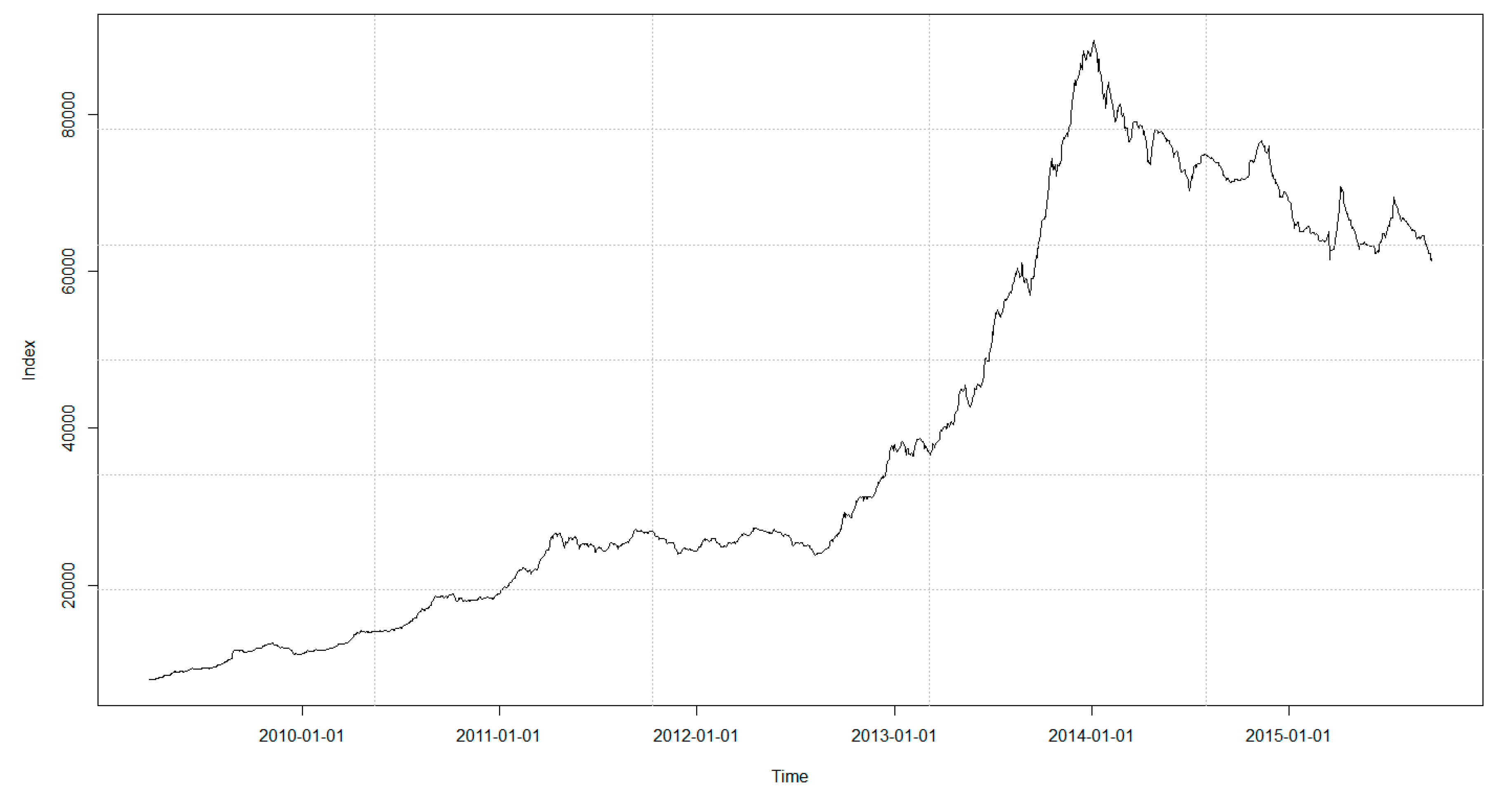
To review the correlation and the fat-tail feature of the data, the plot for the overall index of the Tehran Stock Exchange, for the whole period under consideration, is illustrated in Figure 2.

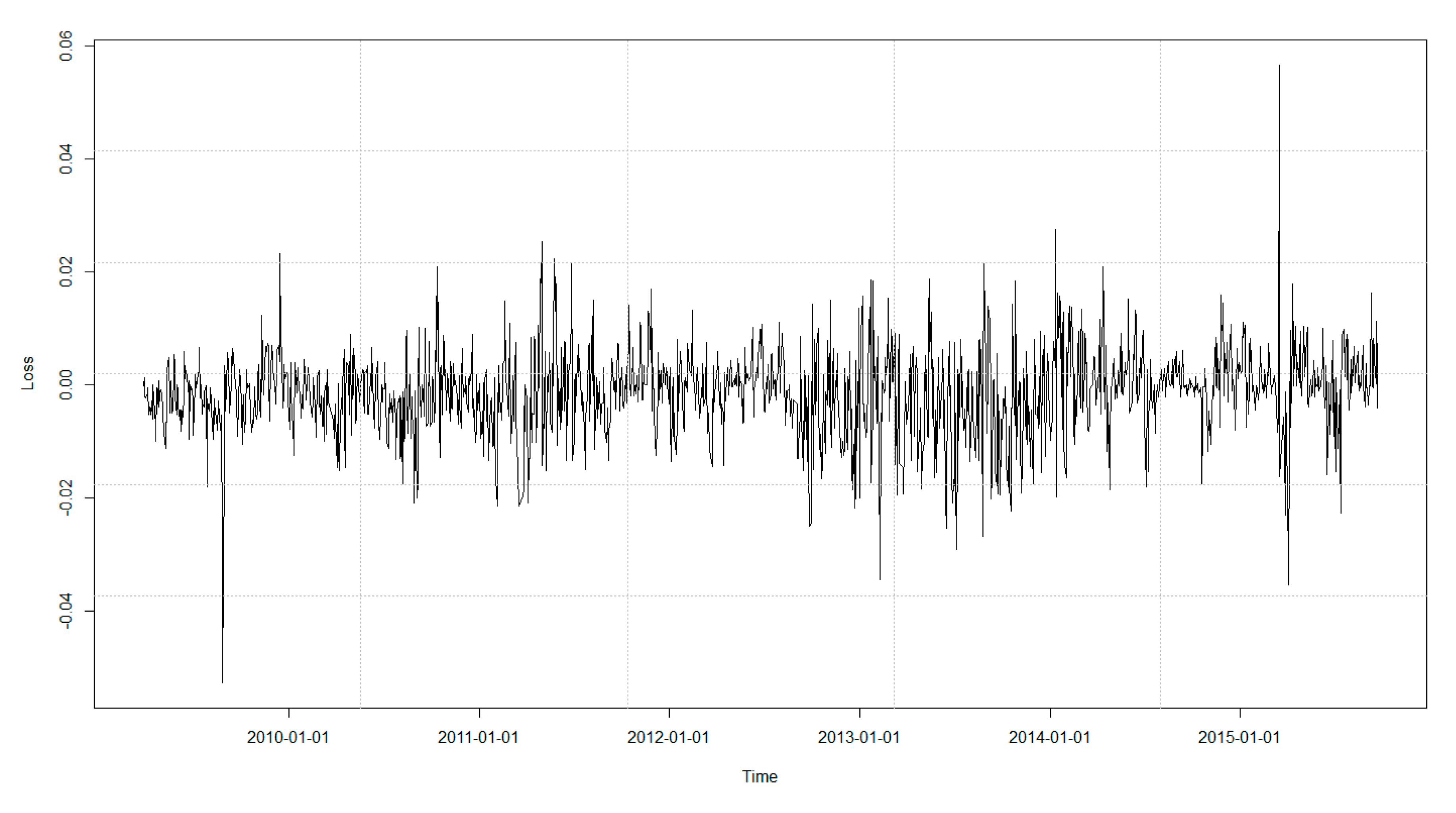
Capital depression period of the Tehran Stock Exchange started in beginning of 2014. For a better understanding of the features of the data in use, the plot for the index return was also investigated, which is illustrated in Figure 3.

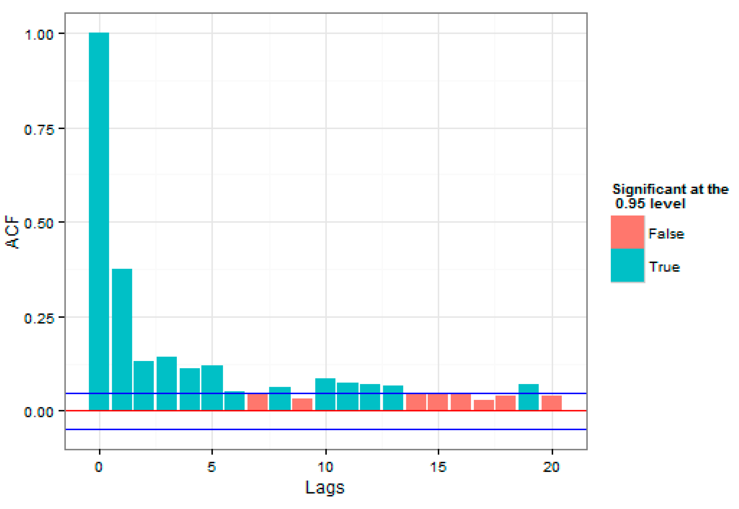
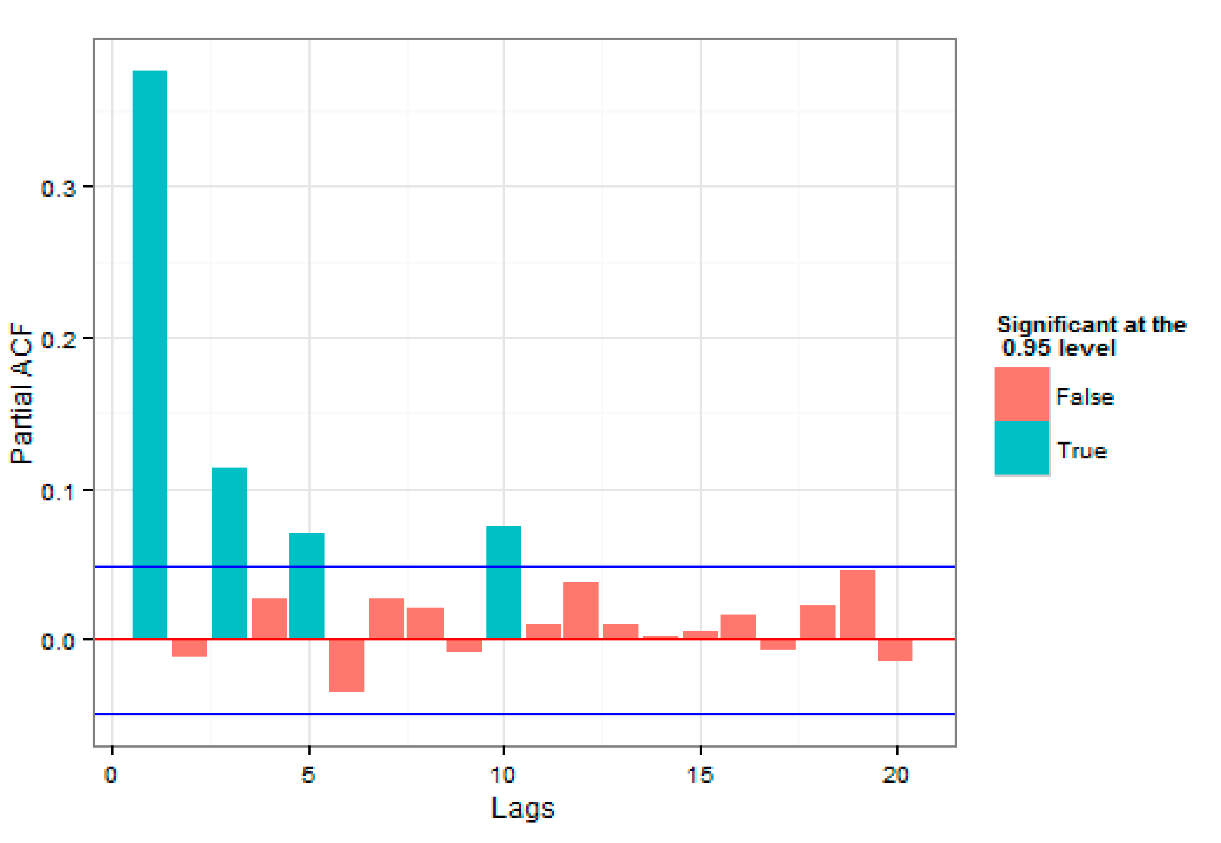
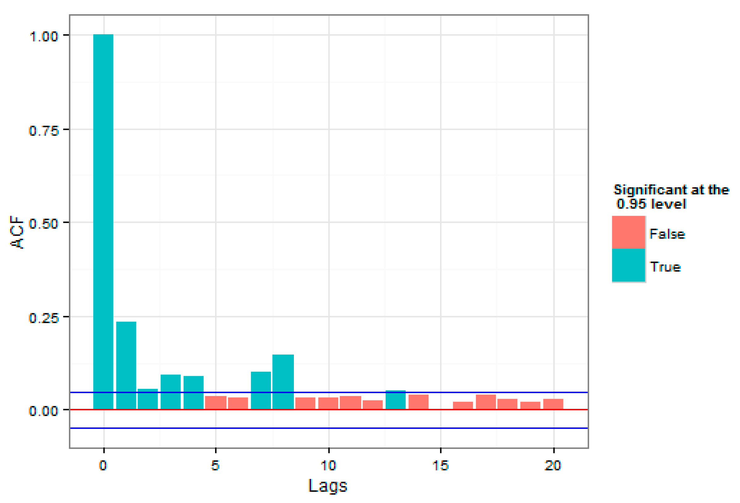
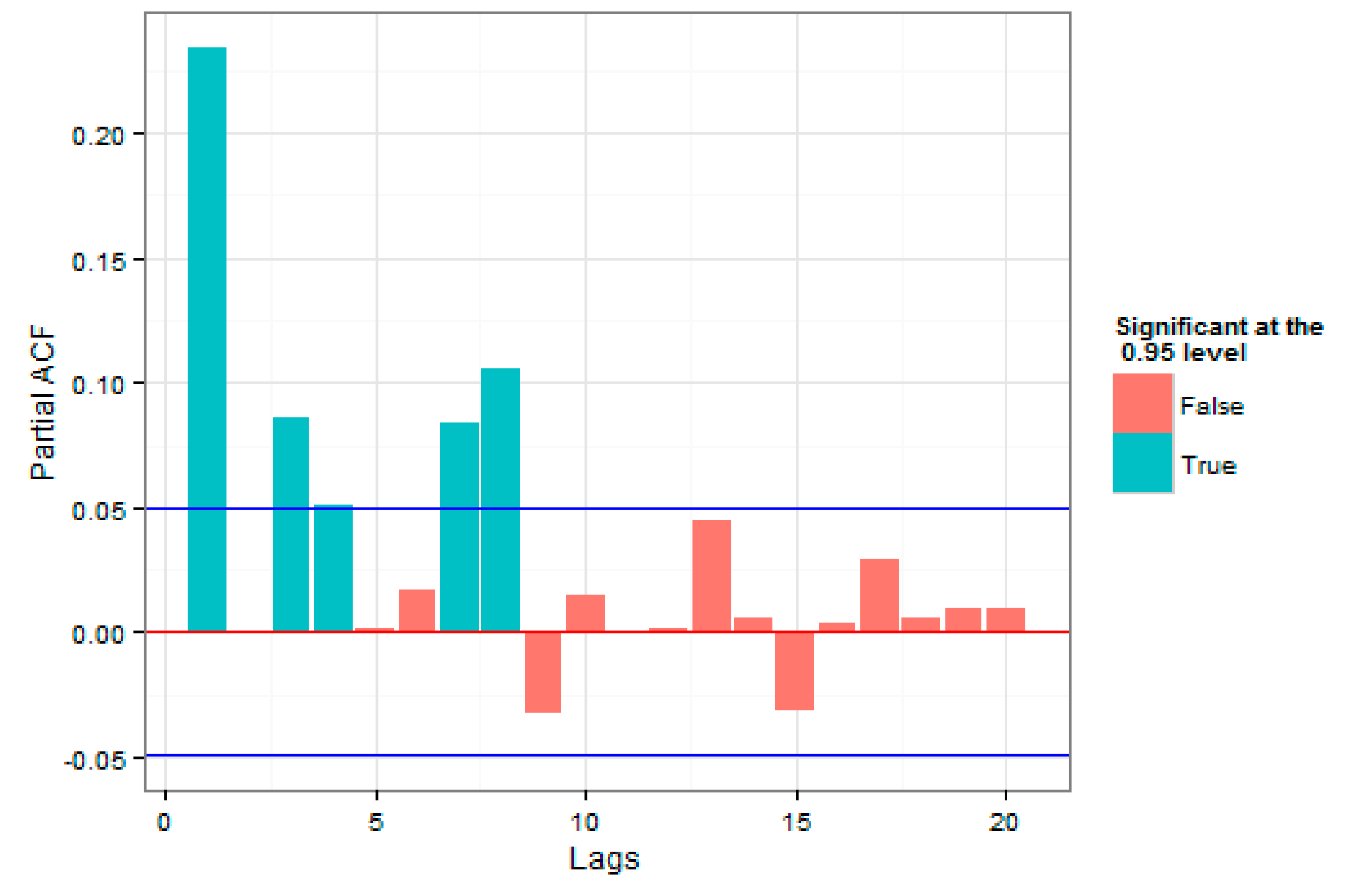
As is evident in Figure 1 and Figure 2, high and low volatilities could be observed for a significant period of time, which was an evidence of correlation with the past data. In addition to correlation in the series under consideration, high volatilities and low volatilities in the loss series were close to each other, which indicated volatility clustering that could justify the use of the GARCH model. To investigate the presence of correlation in the index return series, the autocorrelation and partial autocorrelation plots in Figure 4 and Figure 5 were studied.

In Figure 4 and Figure 5, the number of autocorrelations were studied for different delays, up to 20 period delays. The straight lines at the top and the bottom indicate 2 standard deviations for the standard error of estimation, which approximately showed a 95% confidence level. Both plots were indicative of the presence of autocorrelation in the raw series of returns.

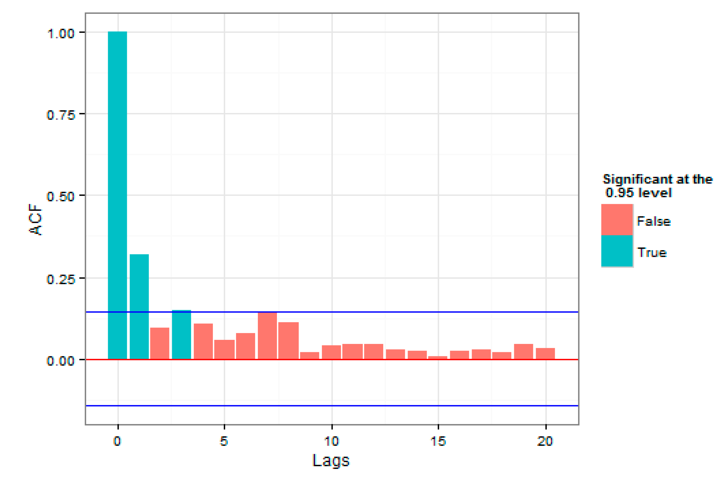
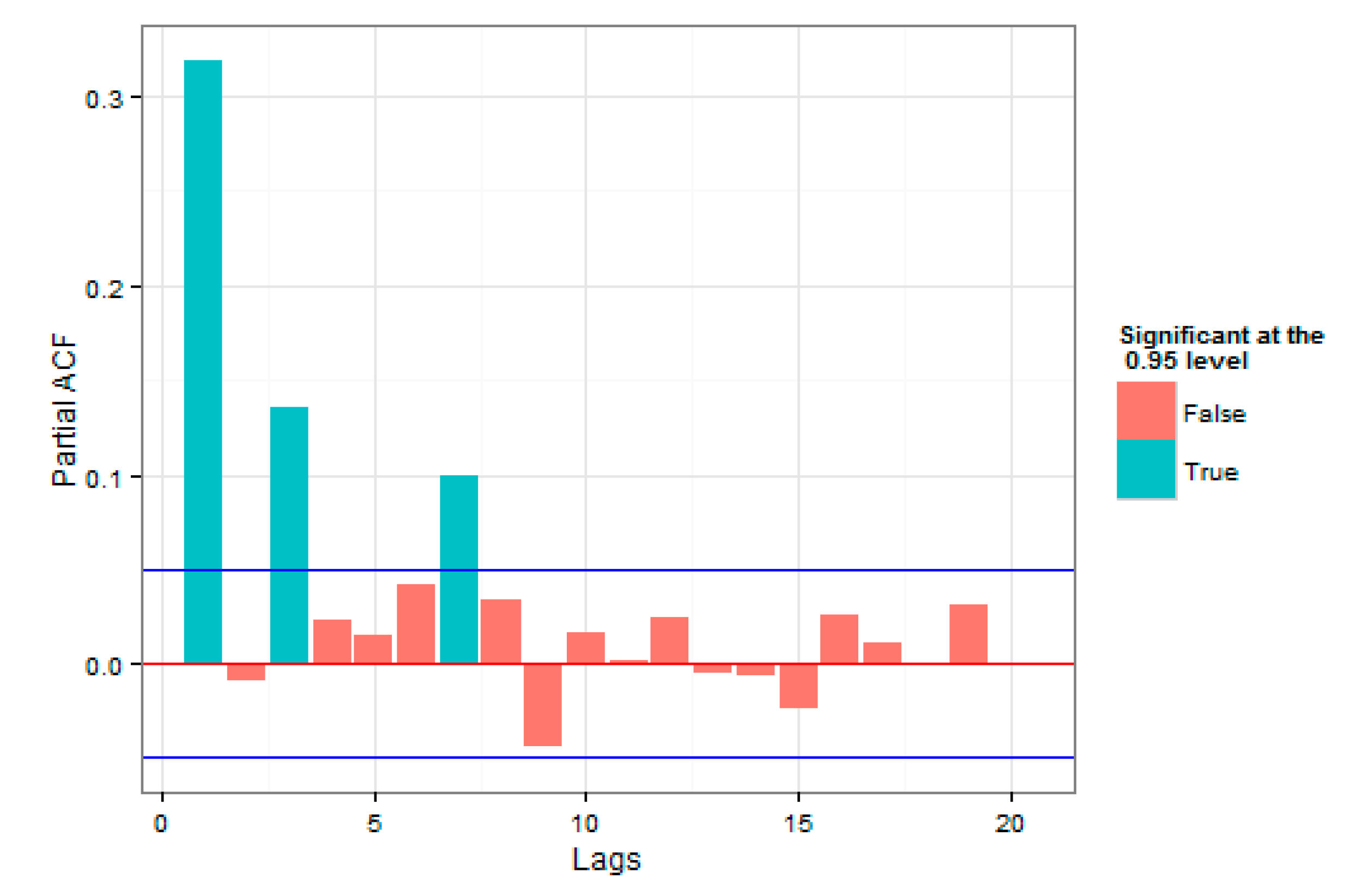
The autocorrelation and partial autocorrelation plots were also been studied for the square of returns in Figure 6 and Figure 7. A review on autocorrelation and partial autocorrelation plots for the square of returns was important, since if the square of returns were considered as an approximation of series volatilities, using the models that utilized volatility correlation was more appropriate.

As was evident, time autocorrelations were also observed in the index returns and this approved the practical studies, regarding the presence of volatility time autocorrelations in the return series.

A review on the plots of autocorrelation and partial autocorrelation of the residual values series, shown in Figure 8, and squares of the residual values series, presented in Figure 9, were also a good guide in using return correlation and volatility correlation models. Since, based on the two figures, return correlation belonged to lower orders; here only one plot, regarding the squares of residual values series of one of the models, was presented.

As was evident, compared to the loss squares plot, it could be stated that the correlations were sufficiently considered by the GARCH model; therefore, after regressing the said mean-variance models, the Extreme Value Theory could be used for the estimation of the Expected Shortfall and the Value at Risk.

The autocorrelation and partial autocorrelation plots have been shown for the square of returns in Figure 6 and Figure 7, suggesting the use of GARCH models, as it was evident, compared to the loss of the squares plot, it could be stated that the correlations were sufficiently considered by the GARCH model. We think volatility clustering existed in the Tehran Stock exchange because of the traders’ behavior and the strong presence of more retail traders than intuitional investors, and the tendency of having a short-term view due to political news and changing regulations. We think the trend was visible and will be repeated in the future. For Iran’s economy, it means that, as volatility clustering is present, it might be difficult for companies to raise capital, as investors are short-term traders, due to many different reasons. There is also no capital gain tax in Iran, which encourages investors to hold the assets for a very short term and react to the news instead of looking to make a fundamental change in the company.

The existence of the volatility clustering feature is expected in the Tehran stock exchange as the number of retail investors (‘chartist’) is significantly high, relative to the number of institutional investors (‘fundamentalist’). One could argue that as the Tehran Stock Exchange is highly isolated and Iran’s economy has experienced very different regimes and cycles, particularly in the periods when sanctions were imposed (first during Barak Obama’s US presidency and later during Donald Trump’s US presidency) and when sanctions were lifted (last two years of Obama’s presidency). We believe that these different economic regimes with a combination of a huge number of retail investors who switched their behavior very quickly, led to large aggregate fluctuations in the context of the Iranian financial markets, and as a result, volatility clustering was seen in the Tehran Stock market.

As described above, we have used the Maximum Likelihood method to estimate the parameters of the Generalized Pareto Distribution (GPD). The maximum likelihood estimates of the left tail of innovation distribution index $\widehat{\xi }$ and the scale parameter $\widehat{\sigma }$, with the corresponding standard errors are presented in

Table 2. Maximum Likelihood Estimates (MLE) of the parameters of Generalized Pareto Distribution (GPD).

Tail	$\widehat{\mathit{\xi }}$	$\mathit{S}\mathit{e}(\mathit{\xi })$	$\widehat{\mathit{\sigma }}$	$\mathit{s}\mathit{e}(\mathit{\sigma })$
Tehran Stock Exchange	0.22	0.108	1.5	0.371

. The estimated tail index $\xi$ of GPD was positive, indicating that the market experienced severe crashes and the probability of occurrence of extreme losses was higher than what the normal distribution predicted. In the case of $\xi$, including the confidence bounds, it was clearly found to be less than 1; there was strong evidence that the usage of a GPD-based expected shortfall was sound.

We have conducted an augmented Dickey–Fuller test on the residuals of the fitted GPD model, over time. As shown in the table below (

Table 3. Dickey–Fuller test on the residuals of the fitted GPD model.

Lag	ADF	p Value
No Drift, no trend
0	−3.76	0.0100
1	−2.65	0.0100
2	−2.61	0.0100
3	−2.55	0.0115
4	−2.39	0.0182
5	−2.47	0.0147
With Drift, no trend
0	−4.81	0.0100
1	−3.43	0.0108
2	−3.45	0.0101
3	−3.36	0.0141
4	−3.26	0.0191
5	−3.33	0.0159
With drift and trend
0	−6.09	0.0100
1	−4.37	0.0100
2	−4.37	0.0100
3	−4.39	0.0100
4	−4.18	0.0100
5	−4.48	0.0100

), estimating these parameters over sub-stretches of time, the parameters were found to be constant over time.

7. Conditional Extreme Value Theory

The procedures mentioned above for the Extreme Value Theory were all non-conditional. That is, they were utilized directly, without any adjustments relative to the considered random variable X. The function of Non-Conditional Extreme Value Theory for the prediction of Value at Risk and Expected Shortfall, could be beneficial in the long-term. However, sometimes due to the phenomena observed in the considered variable, we were interested in the Conditional EVT function for some structures. For example, if the random variable could be modeled with a GARCH procedure, there would be a good opportunity to use the Conditional EVT. In this case, we wanted to use the GARCH procedure to describe the random variable’s volatilities, and then use the Extreme Value Theory, to model the residuals. To this end, McNeil and Frey (2000) have introduced the following two-stage procedure:

First, a volatility predicting model must be used for predicting the volatilities, and after an estimation of the model parameters, the residuals must be extracted. It was expected that these errors had the same distributions and were independent of one another. At the end of this stage, there would be estimations of future volatility and expected return available, i.e., ${\sigma }_{t+1}$ and ${\mu }_{t+1}$. Then, the Extreme Value Theory would be used for the standardized errors and, therefore, using the EVT for residuals, some estimates of the Expected Shortfall and Value at Risk (α percentile) would be achieved.

As was mentioned earlier, with the same number as the original models, with an assumption of normal and T-student distribution for the residual values, the correspondent Peak Over Threshold models were also estimated. With the assumption of normal and T-student distribution, α percentile could be extracted from the relative tables. If the Extreme Value Theory was used for the estimation of $Va{R}_q^t(Z)$ and $E{S}_q^t(Z)$, then:

$$Va{R}_q^t(Z)=u+\frac{{\widehat{\sigma }}_{\max }}{{\widehat{\xi }}_{\max }}\left({\left(\frac{1-q}{{\zeta }_u}\right)}^{-{\widehat{\xi }}_{\max }}-1\right)$$

(7)

$$E{S}_q^t(Z)=\frac{Va{R}_q^t(Z)}{1-{\widehat{\xi }}_{\max }}+\frac{{\widehat{\sigma }}_{\max }-{\widehat{\xi }}_{\max }u}{1-{\widehat{\xi }}_{\max }}$$

(8)

where, ${\zeta }_u$ is equal to the probability of the Z variable, being greater than the threshold, u, or in other words ${\zeta }_u=\frac{n_u}{n}$, ${\widehat{\sigma }}_{\max }$ and ${\widehat{\xi }}_{\max }$ are the parameters of the extended Pareto distribution, which were achieved through the Maximum Likelihood method, after the estimation of u in the Peak Over Threshold method.

8. Backtesting Models

After estimation of the Value at Risk and the Expected Shortfall, the validity of these estimations needed to be investigated. This could be achieved through the backtesting models. Considering the nature of the utilized measures, it could be stated that the Value at Risk backtesting models were more in number and were much more famous than the Expected Shortfall backtesting models.

8.1. Value at Risk Models Backtesting

In this study, unconditional coverage test, independent test, and the conditional coverage test were used. The unconditional coverage test is based on the principle that, if the amount of Value at Risk is appropriately estimated, the number of VaR Breaks are equal to the expected VaR Breaks of a Bernoulli variable, with a success probability of α. For the Null Hypothesis test, the Likelihood ratio test would be used, which was calculated as follows:

$$\begin{array}{l}L(\alpha )={\displaystyle \prod _{t=1}^T{p}^{I_t}{(1-p)}^{1-I_t}=p^{T_1}}{(1-p)}^{T_0}={(1-\alpha )}^{T_0}{\alpha }^{T_1}\\ L(\widehat{\alpha })={(\frac{T_0}{T})}^{T_0}.{(\frac{T_1}{T})}^{T_1}\\ L{R}_{UC}=-2[L(\alpha )/L(\widehat{\alpha })]\end{array}$$

(9)

where, T₁ is one of the VaR Breaks and the ratio is compared to distribution percentile, ${\chi }^2(1)$.

For the confidence levels over the Value at Risk, which would entail few observations (in-sample data), instead of using the statistic above, Christoffersen (2012) recommends the calculation of p-value by the Monte Carlo simulation method.

$$p-value=\frac{1}{1000}[1+{\displaystyle \sum _{i=1}^{999}1}\left\{{\widetilde{LR}}_{uc}(i)>L{R}_{uc}\right\}]$$

(10)

8.2. Expected Shortfall Models Backtesting

For backtesting of the Expected Shortfall models, the model presented by McNeil and Frey (2000), titled Standardized exceedance residuals was used, which is stated as follows:

$$r_{t+1}=\frac{x_{t+1}-{\widehat{ES}}_q^t(X_{t+1})}{{\widehat{\sigma }}_{t+1}},if\hspace{0.17em}{x}_{t+1}>{\widehat{VaR}}_q^t$$

(11)

Based on McNeil and Frey’s model, if the calculated Conditional Value at Risk is an unbiased daily loss estimator, the average of the surplus will be zero and, therefore, in the Hypothesis test, the average of standard surplus is assumed to be zero. In their paper, McNeil and Frey introduced the backtesting model statistic. In this study, the non-parametric bootstrap method, introduced by Kjellson (2013) has been recommended for the calculation of amounts of p-value models. This method is based on McNeil and Frey’s model; however, in McNeil and Frey’s model only the statistic of the model was introduced, but in this method, with simulation, the p-value has been calculated. The introduced model by McNeil and Frey, just like the model above, investigates the validity of the Expected Shortfall models. Embrechts et al. (2005) introduced another model, called V, for comparing the function of the Expected Shortfall models, which has been used for rating in this study.

A detailed report of the fitted models have not been presented as we were only interested in backtesting the models.

9. Research Findings

In this section of the study, data analyses and the results of backtesting the Expected Shortfall models have been discussed. This section includes three subsections—first, analyses of the data before estimation, which aimed at an initial review of the research models; second, analyses of the parameters and estimation of the measures; and third, backtesting of the models, which gave us an interpretation of the results.

It must be noted that the validity of the Expected Shortfall models is dependent on a correct estimation of Value at Risk models. In

Table 4. Bootstrap Test for Expected Shortfall Models.

Data	CtP	Ct	CnP	Cn	GtP	Gt	GnP	Gn	StP	St	SnP	Sn
q = 0.95
Overall	0.053	1.000	0.109	0.043	0.050	1.000	0.062	0.051	0.102	1.000	0.047	0.045
Free Float	0.086	0.766	0.015	0.086	0.213	0.848	0.049	0.077	0.192	0.771	0.047	0.078
Industry	0.218	0.834	0.153	0.087	0.225	0.877	0.171	0.055	0.241	0.870	0.072	0.068
Top 50	0.592	0.772	0.185	0.033	0.619	0.764	0.132	0.040	0.537	0.827	0.065	0.035
q = 0.975
Overall	0.184	1.000	0.250	0.001	0.229	1.000	0.160	0.001	0.312	1.000	0.110	0.001
Free Float	0.213	0.797	0.125	0.001	0.217	0.678	0.178	0.002	0.226	0.796	0.046	0.001
Industry	0.326	0.937	0.267	0.007	0.304	0.877	0.206	0.009	0.360	0.861	0.202	0.003
Top 50	0.546	0.637	0.248	0.010	0.483	0.774	0.208	0.008	0.499	0.718	0.262	0.011
q = 0.99
Overall	0.165	1.000	0.049	0.001	0.059	1.000	0.056	0.001	0.053	1.000	0.051	0.001
Free Float	0.065	0.654	0.011	0.001	0.029	0.423	0.025	0.001	0.033	0.424	0.047	0.001
Industry	0.061	0.719	0.024	0.001	0.081	0.757	0.047	0.002	0.046	0.738	0.041	0.001
Top 50	0.034	0.245	0.033	0.001	0.142	0.398	0.072	0.001	0.083	0.352	0.061	0.001
q = 0.995
Overall	0.043	0.300	0.045	0.001	0.073	0.635	0.066	0.001	0.093	0.536	0.086	0.001
Free Float	0.035	0.121	0.030	0.001	0.014	0.190	0.006	0.001	0.004	0.094	0.006	0.001
Industry	0.068	0.684	0.057	0.001	0.061	0.815	0.044	0.001	0.049	0.777	0.039	0.001
Top 50	0.055	1.000	0.036	0.001	0.112	1.000	0.011	0.001	0.071	1.000	0.009	0.001

, the results of McNeil and Frey’s Bootstrap backtesting is presented. If the p-value was higher than the chosen confidence level, the null hypothesis was not rejected and it approved the validity of the model. The level of error of backtesting was considered to be 0.05. It must be noted, here, that the lack of rejection of the null hypothesis meant the validity of the model was approved. To investigate the validity of the model more critically, the level of error must be raised.

Where, S refers to the simple GARCH models, G refers to the GRJ GARCH models, and C refers to the component GARCH model. Letters n and t show the assumption of a normal and a T-student distribution for the residual values of the model, respectively, and P is the correspondent Peak Over Threshold model of the models above.

As is evident from Table 4, the null hypothesis has been rejected in all of the Expected Shortfall models, with the assumption of a normal distribution. The results of this study were analogous to that of McNeil and Frey (2000), where the authors pointed out that the normal distribution assumption for the residual values in the estimation of Expected Shortfall, was not appropriate. Using EVT in the Expected Shortfall models, with the assumption of a normal distribution for the residual values led to an improvement in the p-value; however, in most cases, the null hypothesis was been rejected at the 5% level.

10. Conclusions

As described in the research literature and data analyzing section, in this study, we have worked on the tail of a non-normal distribution, asymmetric with observed heteroscedasticity characteristics. These characteristics convinced us to use both the GARCH and the EVT models, in order to have a more accurate estimation of the tail of the distribution. We have applied different GARCH models, in combination with the POT (Peak Over Threshold) model, assuming normal or t-distributions for the residual values.

The results of backtesting the Expected Shortfall models at a 5% error level, for all of the levels of Expected Shortfall, are presented in

Table 5. The Results of Backtesting the Models.

Rating	Description	Value at Risk	Expected Shortfall
2	Peak Over Threshold GARCH with a T-student distribution for residual values	Green	Green
4	GARCH with a T-student distribution for residual values	Green	Green
6	Peak Over Threshold GARCH with a normal distribution for residual values	Green	White
8	GARCH with a normal distribution for residual values	Red	Red

, based on their ratings.

To interpret the table above, we must consider the color green as acceptable performance by the model, the color white as nearly acceptable performance (using a conservative model), and color red as an unacceptable performance by the model in the backtesting of the Expected Shortfall models. This categorization is based on the plurality of rejection of null hypothesis at different confidence levels of different indices; meaning that models with more than 70% of no rejection of null hypothesis have been highlighted in green, models with 50% to 70% of no rejection of null hypothesis are in white, and the models with less than 50% of no rejection of null hypothesis are in red. The achieved results can be summarized as follows. Using the normal distribution function for the residual values to estimate Expected Shortfall was not successful and led to an underestimation of risk. Using the T-student distribution in the estimation of the mentioned risk measures, had an acceptable performance, even though in some cases it led to an overestimation of the risk. Consideration of the Extreme Value Theory in the said models, in most cases, led to an improved performance of the model. That is, it had adjusted over- and underestimations, in most cases. Among the GARCH models, the number of successful GJR GARCH models, which model asymmetry in the ARCH process, have been more than that of the other models.

As the data showed the existence of volatility clustering and the essential use of the GARCH model in measuring the market risk by regulators, as per practitioners and academics in research, we suggest that market regulators avoid changing the trading regulations, such as a change in the margin levels (in future contracts) or regulations in the stock lending margin by brokers, which might have exacerbated the uncertainty in the market. We also suggest the use of EVT, based on expected shortfall, in order to measure and manage the market risk in certain instruments, such as future contracts.

Utilizing the POT model had a positive impact on the models and on the estimation of risk, in the financial market. One application of this result could be applying POT to have a more accurate estimation of the initial margin of future contracts, on shares in the Tehran Stock Exchange. For future studies, we suggest the use of other alternative models such as different GARCH models and Neural Network models, assuming an asymmetric distribution for the residual values and modeling, other than financial data characteristics, such as multi-fractality.

References

- Abad, Pilar, Sonia Benito, and Carmen López. 2014. A comprehensive review of Value at Risk methodologies. The Spanish Review of Financial Economics 12: 15–32. [Google Scholar] [CrossRef]
- Artzner, Philippe, Freddy Delbaen, Jean-Marc Eber, and David Heath. 1999. Coherent Measures of Risk. Mathematical Finance 9: 203–28. [Google Scholar] [CrossRef]
- Balkema, August A., and Laurens De Haan. 1974. Residual life time at great age. The Annals of Probability 2: 792–804. [Google Scholar] [CrossRef]
- BCBS. 2012. Fundamental Review of the Trading Book. Basel Committee on Banking Supervision. Consultative Document, May 3. [Google Scholar]
- BCBS. 2016. Minimum Capital Requirements for Market Risk. Basel Committee on Banking Supervision. Standards, January 3. [Google Scholar]
- Bee, Marco, and Luca Trapin. 2018. Estimating and Forecasting Conditional Risk Measures with Extreme Value Theory: A Review. Risks 6: 45. [Google Scholar] [CrossRef]
- Bhattacharyya, Malay, and Gopal Ritolia. 2008. Conditional VaR using EVT–Towards a planned margin scheme. International Review of Financial Analysis 17: 382–95. [Google Scholar] [CrossRef]
- Bob, Ngoga Kirabo. 2013. Value-Atrisk Estimation: A GARCH-EVT-Copula Approach. Master’s thesis, Stockholm University, Stockholm, Sweden. [Google Scholar]
- Brooks, Chris, A.D. Clare, John W. Dalle Molle, and Gita Persand. 2005. A comparison of extreme value theory approaches for determining value at risk. Journal of Empirical Finance 12: 339–52. [Google Scholar] [CrossRef]
- Carr, Nicholas. 2014. Reassessing the Assessment: Exploring the Factors That Contribute to Comprehensive Financial Risk Evaluation. Ph.D. thesis, Department of Personal Financial Planning, Kansas State University, Manhattan, KS, USA. [Google Scholar]
- Chatterjee, Kajal, Edmundas Zavadskas, Jolanta Tamošaitienė, Krishnendu Adhikary, and Samarjit Kar. 2018. A Hybrid MCDM Technique for Risk Management in Construction Projects. Symmetry 10: 46. [Google Scholar] [CrossRef]
- Chen, James Ming. 2018. On Exactitude in Financial Regulation: Value-at-Risk, Expected Shortfall, and Expectiles. Risks 6: 61. [Google Scholar] [CrossRef]
- Chen, Chen-Yu, Jian-Hsin Chou, Hung-Gay Fung, and Yiuman Tse. 2017. Setting the futures margin with price limits: the case for single-stock futures. Review of Quantitative Finance and Accounting 48: 219–37. [Google Scholar] [CrossRef]
- Christoffersen, Peter F. 2012. Elements of Financial Risk Management. Cambridge: Academic Press. [Google Scholar]
- Corbetta, Jacopo, and Ilaria Peri. 2018. Backtesting lambda value at risk. The European Journal of Finance 24: 1075–87. [Google Scholar] [CrossRef]
- Cotter, John. 2001. Margin exceedences for European stock index futures using extreme value theory. Journal of Banking & Finance 25: 1475–502. [Google Scholar]
- Danielsson, Jon, and Casper G. De Vries. 2000. Value-at-risk and extreme returns. Annales d’Economie et de Statistique 60: 239–70. [Google Scholar] [CrossRef]
- Du, Zaichao, and Juan Carlos Escanciano. 2016. Backtesting expected shortfall: accounting for tail risk. Management Science 63: 940–58. [Google Scholar] [CrossRef]
- Embrechts, Paul, Roger Kaufmann, and Pierre Patie. 2005. Strategic long-term financial risks: Single risk factors. Computational Optimization and Applications 32: 61–90. [Google Scholar] [CrossRef]
- Gencay, Ramazan, and Faruk Selcuk. 2004. Extreme value theory and Value-at-Risk: Relative performance in emerging markets. International Journal of Forecasting 20: 287–303. [Google Scholar] [CrossRef]
- Ghorbel, Ahmed, and Abdelwahed Trabelsi. 2008. Predictive performance of conditional extreme value theory in value-at-risk estimation. International Journal of Monetary Economics and Finance 1: 121–48. [Google Scholar] [CrossRef]
- Guegan, Dominique, and Bertrand K. Hassani. 2018. More accurate measurement for enhanced controls: VaR vs. ES? Journal of International Financial Markets, Institutions and Money 54: 152–65. [Google Scholar] [CrossRef]
- Hussain, Saiful Izzuan, and Steven Li. 2018. The dependence structure between Chinese and other major stock markets using extreme values and copulas. International Review of Economics & Finance 56: 421–37. [Google Scholar]
- Iqbal, Shahid, Rafiq M. Choudhry, Klaus Holschemacher, Ahsan Ali, and Jolanta Tamošaitienė. 2015. Risk management in construction projects. Technological and Economic Development of Economy 21: 65–78. [Google Scholar] [CrossRef]
- Jorion, Philippe. 2009. Risk management lessons from the credit crisis. European Financial Management 15: 923–33. [Google Scholar] [CrossRef]
- Kao, Tzu-chuan, and Chu-hsiung Lin. 2010. Setting margin levels in futures markets: An extreme value method. Nonlinear Analysis: Real World Applications 11: 1704–13. [Google Scholar] [CrossRef]
- Kiesel, Rüdiger, Robin Rühlicke, Gerhard Stahl, and Jinsong Zheng. 2016. The Wasserstein metric and robustness in risk management. Risks 4: 32. [Google Scholar] [CrossRef]
- Kilai, Mutua, Anthony Gichuhi Waititu, and Anthony Wanjoya. 2018. Modelling Kenyan Foreign Exchange Risk Using Asymmetry Garch Models and Extreme Value Theory Approaches. International Journal of Data Science and Analysis 4: 38. [Google Scholar] [CrossRef][Green Version]
- Kjellson, Benjamin. 2013. Forecasting Expected Shortfall: An Extreme Value Approach. Bachelor’s thesis, Faculty of Science, Mathematical Statistics Lund University, Lund, Sweden. [Google Scholar]
- Kourouma, Lancine, Denis Dupre, Gilles Sanfilippo, and Ollivier Taramasco. 2010. Extreme Value at Risk and Expected Shortfall During Financial Crisis. Available online: https://papers.ssrn.com/sol3/papers.cfm?abstract_id=1744091 (accessed on 24 May 2019).
- Longin, Francois M. 1999. Optimal margin level in futures markets: Extreme price movements. Journal of Futures Markets: Futures, Options, and Other Derivative Products 19: 127–52. [Google Scholar] [CrossRef]
- McNeil, Alexander J., and Rüdiger Frey. 2000. Estimation of tail-related risk measures for heteroscedastic financial time series: An extreme value approach. Journal of Empirical Finance 7: 271–300. [Google Scholar] [CrossRef]
- Omari, Cyprian O., Peter N. Mwita, and Antony G. Waititu. 2017. Using Conditional Extreme Value Theory to Estimate Value-at-Risk for Daily Currency Exchange Rates. Journal of Mathematical Finance 7: 846–70. [Google Scholar] [CrossRef][Green Version]
- Omari, Cyprian O., Peter N. Mwita, and Antony W. Gichuhi. 2018. Currency Portfolio Risk Measurement with Generalized Autoregressive Conditional Heteroscedastic-Extreme Value Theory-Copula Model. Journal of Mathematical Finance 8: 457–77. [Google Scholar] [CrossRef][Green Version]
- Paul, Samit, and Prateek Sharma. 2017. Improved VaR forecasts using extreme value theory with the Realized GARCH model. Studies in Economics and Finance 34: 238–59. [Google Scholar] [CrossRef]
- Pflug, Georg Ch. 2000. Some remarks on the value-at-risk and the conditional value-at-risk. In Probabilistic Constrained Optimization. Boston: Springer, pp. 272–81. [Google Scholar]
- Pickands, James, III. 1975. Statistical inference using extreme order statistics. The Annals of Statistics 3: 119–31. [Google Scholar]
- Rockafellar, R. Tyrrell, and Stanislav Uryasev. 2002. Conditional value-at-risk for general loss distributions. Journal of Banking & Finance 26: 1443–71. [Google Scholar]
- Soltane, Héla Ben, Adel Karaa, and Makram Bellalah. 2012. Conditional VaR Using GARCH-EVT Approach: Forecasting Volatility in Tunisian Financial Market. Journal of Computations & Modelling 2: 95–115. [Google Scholar]
- Stephenson, Alec G., and Janet E. Heffernan. 2012. ismev: An Introduction to Statistical Modeling of Extreme Values. R Package Version 1. Available online: https://cran.r-project.org/web/packages/ismev/ismev.pdf (accessed on 24 May 2019).
- Stoyanov, Stoyan, Lixia Loh, and Frank J. Fabozzi. 2017. How fat are the tails of equity market indices? International Journal of Finance & Economics 22: 181–200. [Google Scholar]
- Tamošaitienė, Jolanta, Zenonas Turskis, and Edmundas Kazimieras Zavadskas. 2008. Modeling of contractor selection taking into account different risk level. Paper presented at the 25th International Symposium on Automation and Robotics in Construction (ISARC 2008): Selected Papers, Vilnius, Lithuania, June 26–29; Vilnius: Technika, pp. 676–81. [Google Scholar]
- Tamošaitienė, Jolanta, Edmundas Kazimieras Zavadskas, and Zenonas Turskis. 2013. Multi-criteria risk assessment of a construction project. Procedia Computer Science 17: 129–33. [Google Scholar] [CrossRef]
- Thim, Chan Kok, Mohammad Nourani, and Yap Voon Choong. 2012. Value-at-risk and conditional Value-at-risk estimation: A comparative study of risk performance for selected Malaysian sectoral indices. Paper presented at the 2012 International Conference on Statistics in Science, Business and Engineering (ICSSBE), Langkawi, Malaysia, September 10–12. [Google Scholar]
- Wickham, Hadley. 2009. Ggplot2: Elegant Graphics for Data Analysis. New York: Springer. [Google Scholar]
- Wuertz, Diethelm, and Yohan Chalabi. 2010. timeSeries: Rmetrics—Financial Time Series Objects. R Package Version 2110.87. Available online: https://cran.r-project.org/web/packages/timeSeries/index.html (accessed on 24 May 2019).
- Wuertz, Diethelm, Yohan Chalabi, and M. Miklovic. 2009. fGarch: Rmetrics-Autoregressive Conditional Heteroskedastic Modelling. R Package Version 2110. Available online: https://cran.r-project.org/web/packages/fGarch/fGarch.pdf (accessed on 24 May 2019).
- Yousefi, Vahidreza, Siamak Haji Yakhchali, Jonas Šaparauskas, and Sarmad Kiani. 2018. The Impact Made on Project Portfolio Optimisation by the Selection of Various Risk Measures. Engineering Economics 29: 168–75. [Google Scholar] [CrossRef]
- Yu, Wenhua, Kun Yang, Yu Wei, and Likun Lei. 2018. Measuring Value-at-Risk and Expected Shortfall of crude oil portfolio using extreme value theory and vine copula. Physica A: Statistical Mechanics and Its Applications 490: 1423–33. [Google Scholar] [CrossRef]
- Zavadskas, Edmundas Kazimieras, Zenonas Turskis, and Jolanta Tamošaitiene. 2010. Risk assessment of construction projects. Journal of Civil Engineering and Management 16: 33–46. [Google Scholar] [CrossRef]
© 2019 by the authors. Licensee MDPI, Basel, Switzerland. This article is an open access article distributed under the terms and conditions of the Creative Commons Attribution (CC BY) license (http://creativecommons.org/licenses/by/4.0/).