Marketplace Location Decision Making and Tourism Route Planning

Abstract

This research addresses the problem of planning tourism routes and finding appropriate shopping (market place) locations for agricultural product transportation. Generally, tourists visit popular tourism attractions; and generally, unpopular tourism attractions do not stimulate the economy, trade, or local income. Popular tourism attractions that are located far away from each other require the transportation of local products, and tourists must make decisions as to which locations to visit when planning their vacation. Planning a tourism route while balancing tourism attractions and shopping markets is important for the economic stimulation of tourism. This work presents a problem-solving method for tourism route-planning for a particular case study in Chiang Rai province, Thailand, using the Adaptive Large Neighborhood Search (ALNS) method. Six main destruction and five repair cycles in the ALNS method were applied to solve the tourism route design problem and to find the best solution so that tourists can visit all of the main attractions. We found that 13 tourism routes provide the shortest travel distance for each travel route. The total distance traveled was 2538.02 km for all routes. To balance the tourism on all routes, the popular and less popular tourism attractions were combined. For all routes, the shopping market location is the best place for tourism products to be sold and where tourist relaxation occurs. The results from ALNS were compared with the results from those obtained by the exact Lingo program V11. The ALNS algorithm results were not significantly different from the Lingo results. For the computational results for all examined cases, the ALNS algorithm was shown to be competitive, with short processing times given the sizes of the problems. For the traveling distance, the ALNS result significantly differs from the exact method by approximately 1.12%, and had a better effect than the exact method by approximately 99% in terms of processing time. Therefore, the proposed methodology provides an effective and high-quality solution for tourism route planning.

1. Introduction

Tourism management planning is an important challenge in sustainable tourism development. Tourism promotion is a strategy of tourism development that encourages economic development and income for the host country. In many countries, tourism organization involves designed tourism travel routes for popular destinations, but less popular destinations are often not included. Many tourists seek out new tourism attractions to improve their experience. Therefore, the popularity of a tourism attraction is an important consideration when planning travel (Ram et al. 2016). Many popular tourism attractions are crowded with tourists due to these attractions being promoted by tourism organizations. The popularity of the promoted attractions influences various aspects of the community, such as trade and income. However, this development only occurs in the popular tourism areas and less so, or not at all, in the less popular tourism attraction areas, the latter of which are often supported by the government. Less popular tourism attractions have become underdeveloped and are often in disrepair, causing a lack both of income and economic development for the locals. Tourism route management involves important tourism planning decisions that benefit the local economy. In tourism route planning, trades and services are generated by increasing the number of tourists. Tourism route planning has been studied in terms of visitors to popular tourism attractions or to a chosen destination (Yan et al. 2017; Andrades and Dimanche 2017; Souffriau and Vansteenwegen 2010; Kang et al. 2006; Lim et al. 2018). This tourism attraction imbalance means less popular tourism features are not included in the tourism route, resulting in the less popular attractions and less-developed areas to be in rarely-visited areas or difficult-to-reach destinations, respectively. Consequently, tourism must strike a balance between the less popular attractions and more popular attractions in tour route for tourism economic encouragement and development. Tourism promotion improves the popularity of the less popular tourism attractions in terms of development and job creation.

An important responsibility of the tourism department is tourism pattern design, which includes tourism route design, facilities design, and rest locations for tourist support, as tourism experience and satisfaction during a trip are derived from the tourism route that is planned by tourists before they travel to unfamiliar destinations. The design of the tourism route and selection of suitable shopping market locations is important in the development of local trade and tourism attractions. These two aspects are planning problems that require information from tourism organizations and tourists (Nagy and Salhi 2007). This information is employed in the creation of tourism travel plans. Examining travel arrangements is an essential process in tourism planning that includes aspects such as traveling costs, the locations of facilities, time required for travel, the tourist attractions, and the travel route (Flognfeldt 2005). In some cities, the travel problem arises from the lack of travel planning guidance, restaurant/dining information, and tourism route data for each tourism attraction (Gavalas et al. 2014).

Northern Thailand, and the Chiang Rai Province in particular, is a major attraction and has many tourism attractions, including temples, culture, agricultural features, and beautiful natural scenery. Approximately one million tourists visit Chiang Rai each year. Formerly, tourists could not visit all the tourism attractions in Chiang Rai, because Chiang Rai has no route management or facilitated travel. Many tourism attractions are far from each other, limiting the ability to visit many during one holiday. Accordingly, the tourism route should be planned before the visit. The popularity of the tourism attractions was reported by tourists as the main reason for sightseeing. The popular tourism attractions are income generators, creating several forms of employment, such as service, hire, and trading for people, or agriculture, around the popular tourism attractions. The people or farmers who live far from the popular tourism areas are not able to transport their products for sale to the area due to the lack of a market place. Similarly, people or farmers around the less popular tourism attractions have lower income, due to low tourist interest or tourist numbers. Achieving a tourism attraction balance provides economic motivation in Chiang Rai, which can be addressed by solving the tourism design problem caused by the imbalance between popular and less popular tourism activities and sites. In addition, the tourism organization, Chiang Rai Tourism Office, and the local administration consider season, facility, tourism attraction, local identity, and local product sale as key tourism development factors. Marketplace allocation is necessary for tourism trip design for stimulating local economic development and determining tourism routes. The shortage of both tourism planning and locations that facilitate tourism has resulted in tourists being unable to visit all the tourism attractions within their time limit, which may negatively influence the satisfaction of tourists (Lumsdon and Stephen 2004; Zheng et al. 2017). Tourist satisfaction is a problem in tourism trip design (Lu et al. 2016). The tourism trip design problem has only been studied in terms of the Vehicle Routing Problem (VRP) (Gavalas et al. 2014) and the Location Routing Problem (LRP) (Caroline and Christian 2014).

In Chiang Rai, the Tourism Trip Design Problem (TTDP) is becoming an increasingly important problem, and is a combination of three problems: VRP, LRP, and Assignment Problem (AP). LRP involves market place allocation. The market place is a location for coffee shops, restaurants, and/or farm stores, etc. The transport of agricultural products is the problem faced by the farmer. As a result, suitable marketplace locations are important for tourism support. In addition, the tourism time limit was defined as a one-day trip in Chiang Rai, so tourists have about 11 h for traveling and visiting all the tourism attractions, which is a VRP (Alfredo and Omar 2007). The combination of these three aspects creates the overall tourism design problem as a TTDP in Chiang Rai. However, the TTDP is a complex and time-consuming process that involves selecting points of interest as well as the trip route. The large amount of available tourism data means that tourists will spend more time and effort in studying and evaluating the possible alternatives for their holiday trip. Considerable work is required to solve the TTDP problem, which involves planning the route to be traveled and maximizing entertainment while considering numerous constraints (Vansteenwegen and Van Oudheusden 2007; Liu et al. 2014; Rodríguez et al. 2012).

Sirirak et al. (2018) studied the tourism routing problem in Chiang Rai Province, Thailand. They presented a mathematic model for solving the tourism route planning problem using the Lingo program (M-focus Co Ltd, Bangkok, Thailand) with more and less popular attractions ordered for daily balance. They found a suitable solution for a small amount visitation of people, but increasing the number of visited tourism attractions required more time, which could not solve the problem. Boonya and Wisittipanich (2017) presented mathematical models that solved the TTDP using the exact method in the Lingo program for Chiang Mai, Thailand. Traveling plans were formulated with some constraints such as time and cost. The solution attained showed that when the number of attractions increases, the computational time rapidly increases.

However, Thailand has many tourism attractions in several provinces, which the Lingo program could not successfully solve due to the computational complexity. The research on the design of tourism routes is still in its infancy. Therefore, we present the Adaptive Large Neighborhood Search (ALNS) algorithm in this study for solving the TTDP in Chiang Rai Province, Thailand. The tourism route literature was reviewed and is summarized in Section 2. The problem description and mathematical formulation are outlined in Section 3. The ALNS algorithm is introduced in Section 4. The results of and discussion about the Adaptive Large Neighborhood Search algorithm are provided in Section 5, and finally, Section 6 provides our conclusions.

2. Literature Review

The Tourist Trip Design Problem (TTDP) and Tour Route Planning Problem (TRPP) are important problems in tourism. These problems are caused because the tourist cannot visit the all the desired tourist attractions. A long journey and the time window are main limitations when deciding where to go. Therefore, the traveler can visit tourism attractions within the time limit based on the route planned and the facilities available for tourism support. Many studies showed that the success of tourism depends on the route planned and the information that supports tourism decisions. Yan et al. (2014) presented the planning process by studying a quantitative method that could potentially be used for tourism development at heritage sites in China. The authors created a mathematic model of the planning process. The values produced by the model show the priority of the tourism sites, which provides planning information for tourists. The tourism routing information and the restaurant and shopping locations play an important role in the tourist’s route selection when choosing which tourist attractions to visit. Many studies applied the heuristic method to tourism routing in the TRPP and TTDP, which included traveling to famous and far away tourism attractions. A solved tourism trip was reported using the heuristic method based on local search, which provided a good solution and made the best use of the time available for sightseeing. Zhu et al. (2012) solved a tourist trip design problem that included a variation in the time and the environment, such as traveling times or waiting times. The parameters of the mathematical model are deterministic and stochastic time. The problem addressed by Xiao et al. (2017) was single-tour time-dependent stochastic TTDP for optimizing route and time allocation. The combination of genetic algorithm (GA) and differential evolution (DE) was used to solve this TTDP. The algorithm was developed for providing a highly personalized tourism route under varied time and environment. Changing the time and environment affect the sightseeing choice of the tourist, so the algorithm was able to provide traveling support to tourists and improve tourist confidence.

Conflicting and different touristic styles in a group is a modification of the tourism problem (Zhu et al. 2012; Liao and Zheng 2018). Yu et al. presented a mathematical model and algorithms for solving the TTDP using the exact method and heuristic method—the particle swarm optimization (PSO). The proposed method maximized the attraction’s total collected score, meaning each tourism attraction can be visited once at most. The solved TTDP provided an optimal route for the tourist trip design plan (TTDP) in transport vehicles (Yu et al. 2014). Wu et al. (2017) presented a tour route planning problem (TRPP) solution using a greedy construction procedure for creating a route planning model that maximized the tourism experience utility, considering tourists’ preferences in terms of attraction, traveling time, and traveling cost. Tourism visits were time-constrained from 8:30 a.m. until 4:40 p.m. and limited to 200 yuan per day. The popularity of the tourism attraction was important for the tourism route plan. The MATLAB program was used for the solution algorithm. The results of the problem solving showed that suitability of attractions, degree of interest, tourism time, and tourism cost considerably influenced the tour route plan. However, traffic significantly impacted traveling time on the route (Wu et al. 2017). Similarly, Yan et al. (2014) developed a tour route to optimize satisfaction and minimize route distance. The problem was solved using the PSO method. The constraints on the tourism route design problem were cost, tourism attraction, and walking and tour time. The PSO algorithm can be used to solve the problem of tour route design, the result of which is tour route for tourists. However, the effect of tourism attraction congestion on the tourist satisfaction of sightseeing was not considered (Yan et al. 2014). In addition, Xiao et al. (2017) used the neural net buffer algorithm to support tourism route planning in Zhengzhou, China. The popular attractions were classified into sight-seeing locations, the number of the tourism attractions, and the sightseeing time limit to generate a multi-perceptron (MP) nerve cell route planning model. The model was feasible and valuable and can provide effective decision support for tourists (Xiao et al. 2017).

Although many methods effectively solved the tourism route design problem and travel route planning problem, the above-mentioned methods such as GA, DE, or PSO may not provide the best solution. This is the next step in tourism route planning solution improvement. One method that could potentially improve the solution is the Adaptive Large Neighborhood Search (ALNS) method. ALNS does not need to improve the solution after problem solving because the ALNS method can be implemented within problem solving process. ALNS has been used to solve other problems such as the Vehicle Routing Problem, Location Routing Problem, and the Tourism Routing Problem (Dayarian et al. 2016; Azi et al. 2014; Zajac 2017). ALNS solves these problems well and provides the optimal solution for the vehicle routing problem as well as other problem. Azi et al. (2014) presented the ALNS method for solving the VRP with multi-routes for all customer requests within a time limit on transportation. The proposed solution maximizes the number of served customers and the total distance traveled. The problem was solved using the ALNS algorithm for the customer, the route, the workday level of destroying, the least-cost insertion, and the regret-based insertion of repairing. The served customers and the total distance result were nearly optimum within a 1–2.5% error, which is excellent performance in terms of the computational efficiency and solution quality. Dayarian et al. (2016) used the ALNS algorithm to solve a multi-period VRP with seasonal variations. This problem was solved by optimizing the product group and the redistribution. The formulation process was separated into two stages: the minimization of the total cost of the old plan, and solution adjustment. The comparison of the exact algorithm and the ALNS showed that the exact algorithm was unable to provide an optimal solution for the larger problem, due to the complexity increase caused by the increase in depots. The ALNS computation for all instance sizes provided similar results, but the processing time was shorter. The ALNS method produced high quality solutions with low processing time. However, stochastic demand, such as daily variation in production level, was not studied to improve the solution (Dayarian et al. 2016). Gullhav et al. (2017) presented the solution of multi-tier service deployment problems in clouds using ALNS. Seven destroy and three repair operations were used in the ALNS solution improvement. The results produced by the ALNS algorithm were compared with the results of the branch and price (B&P) method. The call frequency testing showed that the ALNS had similar results to the B&P method. The ALNS method decreased the call iterations by 25–35% for case testing 70 services. The small ALNS instance provided 75% private cloud coverage. For the large instances of ALNS, 50% of the iterations were required. However, the difference in the computation times for the two different methods were not significant for small instances, but the large instances were significantly different (Gullhav et al. 2017).

Chen et al. (2018) studied the dynamic VRP with the ALNS method. The constraints were vehicle and time limits. The destroying ALNS included random removal, worst removal, static-related removal, and time-related removal. The repairing ALNS aspects included greedy insertion, regret insertion, and noise insertion. The comparison of average travel distance with other methods showed that the ALNS results were slightly worse than the others, with less than 4.63% error and short computation time, producing a quality improvement in the solution. Alinaghian and Shokouhi (2018) presented a multi-depot and multi-compartment solution of the vehicle routing problem that minimized both the number of vehicles and the total distance traveled. The results obtained from the exact method Variable Neighborhood Search (VNS) and the hybrid ALNS algorithm were compared. The exact VNS ALNS method and hybrid ALNS produced the best result of all methods, with a slight difference between the two, and ALNS having a shorter average processing time than the exact method, VNS, and hybrid ALNS for large instances. Therefore, the ALNS provided the best formulation and performance in terms of solution finding (Alinaghian and Shokouhi 2018).

The literature demonstrates the effective problem-solving ability of ALNS, which is why we the ALNS method is often chosen for solving tourism route design problems. Although the solution provided by ALNS is not a global solution, the result is statistically accepted by researchers. Therefore, the ALNS method was chosen to solve the tourism route design problem for our case study in Chiang Rai Province in Thailand.

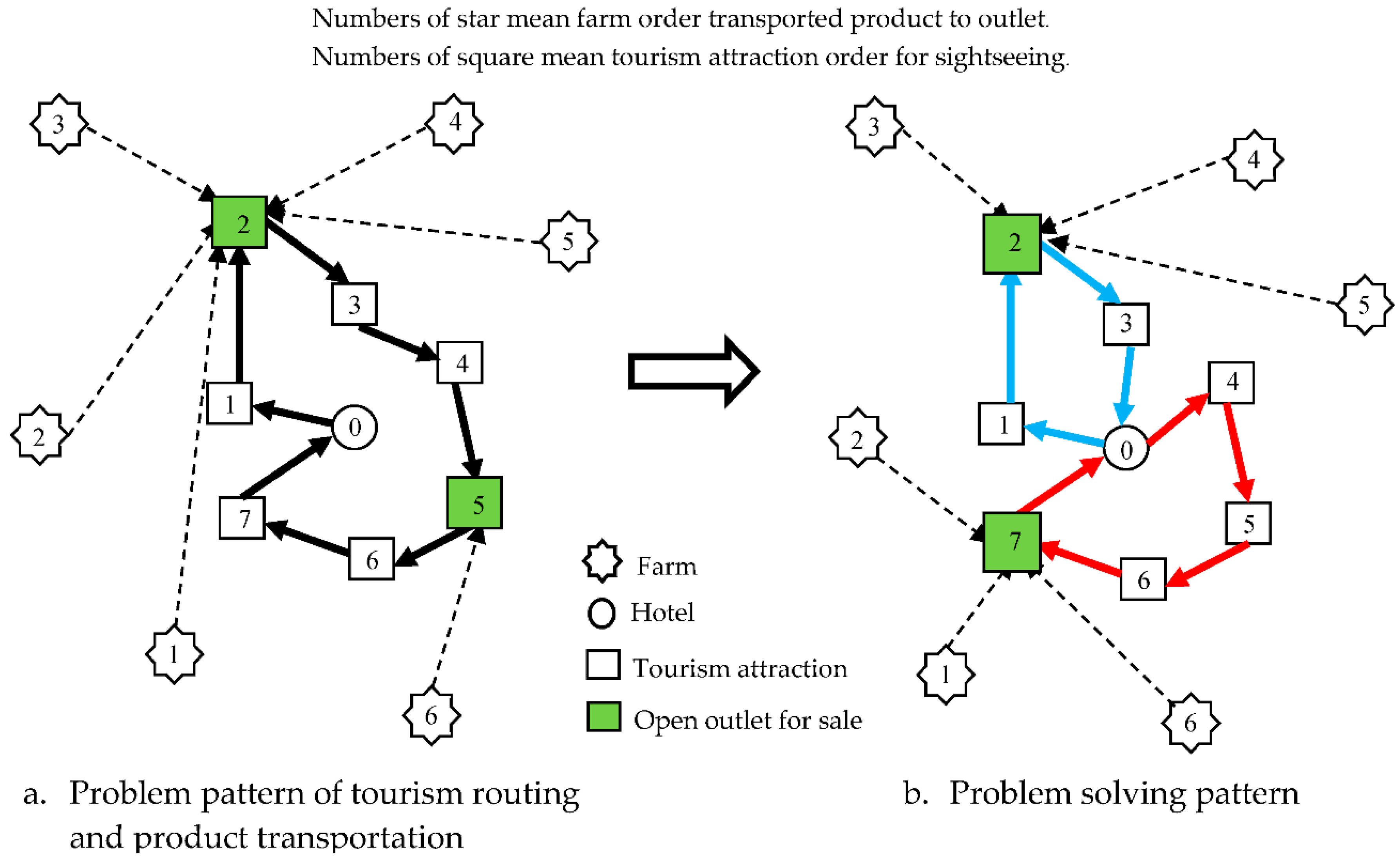
3. Problem Description and Mathematical Formulation

In Chiang Rai, Thailand, the tourism problem is finding a tourism route to visit all desired all tourism attractions. Several popular destinations were chosen as main destinations and as less popular destinations. Traveling route management is a balance of popular and less popular tourism attractions. This was the initial tourism routing problem in Chiang Rai. From the surveyed tourism attraction data, tourists strongly prefer to rest between 11.00 a.m. and 2:00 p.m., but the less popular tourism attractions do not have facilities to support this need, such as coffee shops, shopping outlets, markets, or recreation places. Therefore, tourists choose to not visit these less popular destinations. The local economy was not improved through tourist expenditure. However, these types of places were plentiful around the popular tourism attractions. This is a tourism selection factor: the tourist prioritizes popular tourism attractions. This evidently causes the less popular tourism attraction to be less developed, which negatively affects local income.

The people and farmers who live around the less popular tourism attractions, encounter a problem in terms of employment or local product trade. The people and farmers do not receive enough income from local product commerce. The agricultural products are transported from the farms to the popular tourism attractions, far from the farm but close to tourist crowds. The problem pattern is shown in Figure 1a. The people and farmers incur high cost due to product transportation or product damage. Therefore, the high-cost products decreased as the distance decreased due to traveling route planning that balanced the tourism attractions with suitable shopping outlet locations for both farmers and people. As such, suitable market locations provide economic opportunity for locals and the country. The problem-solving concept patterns are shown in Figure 1b.

The agricultural products are transferred from the farm near the tourism attraction (pickup location), causing a reduction in the transport distance and the cost of the product. Therefore, the problem-solving pattern was summarized as the solving of the tourism, career creation, and income distribution problem. This problem was transformed to mathematical model as shown in Section 3.2. Various studies presented tourism route planning and design for solving the vehicle routing problem or tour trip design problem as shown in

Table 1. Related research of tourism problem.

Study	Topic	Approach									% Gap
		TTN	GA	DE	TS	NNW	PTA	RA	CSCRA	LP
Wang et al. (2018)	Electric vehicle tour planning							✔			0
Lim et al. (2018)	Tour recommendation and itinerary planning						✔				2.5–15
Liao and Zheng (2018)	Tourist trip design problem; TTDP		✔	✔							1.98–13.10
Wu et al. (2017)	Tour route planning problem	✔									-
Nedjati et al. (2017)	Tour location routing problem		✔								-
Kotiloglu et al. (2017)	Multi-period tour				✔						0.04
Zheng et al. (2017)	Design personalized day tour route		✔	✔							3.50–5.85
Xiao et al. (2017)	Tourism route planning					✔					-
Gavalas et al. (2014)	Time-dependent team orienteering problem								✔		3.4–14
Rodríguez et al. (2012)	Development of tool for individual tourists				✔						2.17–4.28
Zhu et al. (2012)	Tour planning problem									✔	0.12–2.84

Note: TTN = Tourism Transportation Network; GA = Genetic Algorithm; DE = Differential Evolution; TS = Tabu Search; NNW = Neural Network; LP = Linear programming; PTA = PersTour Algorithm; RA = Reduction Algorithm; CSCRA = CSCRoutes Algorithm.

.

3.1. Data Collection

The travel route problem solving and the outlet finding started with collecting data from the attraction location and the farm location for product haulage to the sales outlet during the office hours of the tourist attraction in Chiang Rai. The data collected included the following components: locations of tourist attractions, locations of farms, travel time, and open and close time of the attraction or time windows. We used geographic coordinate data for the attraction location, which included latitude and longitude for distance matrix creation. These data were used with Google map data to help determine distance between locations. There were 115 tourism attractions and 25 farms used in this study. The time window of the tourist attraction and the location of the farms are shown in

Table A1. Example of data used for mathematical model tests.

Order	Tourism Attraction	Latitude	Longitude	Open-Close Times
0	Rest	19.925738	99.82364	8:00 a.m.–6:00 p.m.
1	Wat Rong Khun	19.824285	99.763159	7:00 a.m.–6:00 p.m.
2	Boonrod farm	19.852997	99.743386	6:00 a.m.–8:00 p.m.
3	Wat Phra Sing Chiang rai	19.911672	99.830615	8.00 a.m.–6:00 p.m.
4	Wat Phra Kaew	19.91171	99.827718	6:00 a.m.–6:00 p.m.
5	Wat Huai Pla Kha	19.948406	99.806396	7:00 a.m.–6:00 p.m.
. . . .	. . . .	. . . .	. . . .	. . . .
113	Bak International Port	20.275078	100.40596	8.00 a.m.–7:00 p.m.
114	Saturday Night Market	20.25453	100.410303	4.00 a.m.–9.00 p.m.
115	Wat Luang	20.043683	100.379802	8.00 a.m.–6:00 p.m.

and

Table A2. The locations of farms.

Order	Farm	Latitude	Longitude
1	Mae Kao Tom	20.009389	99.912778
2	Mae Kon	19.849194	99.732778
3	Ban Du	19.977111	99.831444
4	Rim Kok	19.985417	99.935472
5	San Sai	19.856694	99.815528
. . . .	. . . .	. . . .	. . . .
23	San Klang	19.592139	99.707333
24	Pa Hung	19.567889	99.702972
25	Wiang Hao	19.525389	99.85355

, respectively.

3.2. Mathematical Model

The tourism problem was complex and difficult because there are many tourism attractions and suitable outlet locations for product transportation. Suitable outlet locations were based on the time constraint. The time constraint was time during which tourists take breaks: 11:00 a.m. to 2:00 p.m. The farmer was assigned product transportation from a start point, and the end of daily travel, as accommodation which 11 h is the maximum time limit of sightseeing tourist. Therefore, the best tourism route ensures the tourist arrives at the attraction during its open time window and traveling the shortest distance within the day while balancing the both popular and less popular tourist attractions for each route. Also, the outlets are located in places suitable for rest. The tourist attraction was scored 1 to 10 in terms of popularity, which was transformed to 1 to 5 stars. From the problem solving pattern in Figure 1b, a mathematical model was created by Sirirak et al. (2018) as follows, where i is the tourist attraction and i is valued in the set I = 1, 2, …, I; j is the tourist attraction and j values in the set J = 1, 2, …, J; k is the outlet location and k is valued in the set K = 1, 2, …, K; and f is the farm that supports the tourism product and f is in the set F = 1, 2, …, F. The decision variables are: X_ij = 1 when the trip goes from the tourist attraction i to tourist attraction j, and 0 otherwise; Y_fj = 1 When delivery occurs from farm f to tourist attraction j, and 0 otherwise; ${\mathrm{R}}_{\mathrm{j}}^1$ = 1 when the outlet at tourist attraction j is open, and 0 otherwise; and ${\mathrm{R}}_{\mathrm{j}}^2$ = 1 when the level of importance of the tourist attraction j is 5 star at the outlet, and 0 otherwise. The parameters are: A = Time spent traveling (min to km), B_k = Earliest allowed arrival time at outlet k (min), C_k = Latest allowed arrival time at outlet k (min), E_k = Time spent visiting at outlet k (min), G = Maximum time spent on each trip(min), H = Maximum number of vehicles (car), U_i = The reward points of each tourist attraction I, W_k = Time of the vehicle to the point of outlet K, M = The capacity of the car in goods transportation to the outlet, S = The tourist attraction was chosen as the location for the product, ${\mathrm{Q}}_{\mathrm{i}}$ = Weight classification points that give attractions, ${\mathrm{D}}_{\mathrm{i}\mathrm{j}}^1$ = Distance from tourist attraction i to tourist attraction j (km), and ${\mathrm{D}}_{\mathrm{f}\mathrm{j}}^2$ = Distance of tourism product shipment from farm f to tourist attraction j (km).

The objective function is the sum of the lowest total traveling distance and product transport distance for tourism route planning for sightseeing within the allowable time window. The objective function is as follows:

$$\mathrm{M}\mathrm{i}\mathrm{n}\mathrm{Z}={\displaystyle \sum _{\mathrm{i}\in \mathrm{I}\cup \mathrm{J}}{\displaystyle \sum _{\mathrm{j}\in \mathrm{I}\cup \mathrm{J}}{\mathrm{D}}_{\mathrm{i}\mathrm{j}}^1}}{\mathrm{X}}_{\mathrm{i}\mathrm{j}}+{\displaystyle \sum _{\mathrm{f}\in \mathrm{F}}{\displaystyle \sum _{\mathrm{j}\in \mathrm{J}}{\mathrm{D}}_{\mathrm{f}\mathrm{j}}^2}}{\mathrm{Y}}_{\mathrm{f}\mathrm{j}}$$

(1)

The research problem has many constraints on problem solving such as traveling time, popular destination level, destination score, etc. The constrained functions of this problem are as follows:

$${\mathrm{X}}_{\mathrm{k}\mathrm{k}}=0\hspace{1em}\hspace{1em}\hspace{1em}\hspace{1em}\hspace{1em}\hspace{1em}\forall \mathrm{k}\in \mathrm{K},\forall \mathrm{k}\in \{1,\mathrm{k}\}$$

(2)

$${\displaystyle \sum _{\mathrm{j}=1}^{\mathrm{J}}{\mathrm{Y}}_{\mathrm{f}\mathrm{j}}}=1\hspace{1em}\hspace{1em}\hspace{1em}\hspace{1em}\hspace{1em}\hspace{1em}\forall \mathrm{f},\mathrm{j}\in \mathrm{F}\mathrm{J}$$

(3)

$${\mathrm{R}}_{\mathrm{i}}^1=0$$

(4)

$${\displaystyle \sum _{\mathrm{j}=1}^{\mathrm{J}}{\mathrm{R}}_{\mathrm{j}}^1}={\displaystyle \sum _{\mathrm{j}=1}^{\mathrm{J}}{\mathrm{X}}_{1\mathrm{j}}}\hspace{1em}\hspace{1em}\hspace{1em}\hspace{1em}\hspace{1em}\hspace{1em}\forall \mathrm{f}\in \mathrm{F},\forall \mathrm{j}\in \mathrm{J}$$

(5)

$${\mathrm{Y}}_{\mathrm{f}\mathrm{j}}\le {\mathrm{R}}_{\mathrm{j}}^1\hspace{1em}\hspace{1em}\hspace{1em}\hspace{1em}\hspace{1em}\hspace{1em}\forall \mathrm{f}\in \mathrm{F},\forall \mathrm{j}\in \mathrm{J}$$

(6)

$${\mathrm{R}}_{\mathrm{j}}^2\ge {\mathrm{R}}_{\mathrm{j}}^1{\mathrm{X}}_{1\mathrm{j}}\hspace{1em}\hspace{1em}\hspace{1em}\hspace{1em}\hspace{1em}\hspace{1em}\forall \mathrm{j}\in \mathrm{J}$$

(7)

$${\mathrm{R}}_{\mathrm{j}}^2\ge {\mathrm{R}}_{\mathrm{i}}^2+{\mathrm{R}}_{\mathrm{j}}^1{\mathrm{X}}_{\mathrm{i}\mathrm{j}}-(1-{\mathrm{X}}_{\mathrm{i}\mathrm{j}})\hspace{1em}\hspace{1em}\hspace{1em}\hspace{1em}\hspace{1em}\hspace{1em}\forall \mathrm{i}\in \mathrm{I},\forall \mathrm{j}\in \mathrm{J}$$

(8)

$${\mathrm{R}}_{\mathrm{i}}^2\le 1$$

(9)

$${\mathrm{T}}_{\mathrm{j}}\ge {\mathrm{S}}_{\mathrm{j}}{\mathrm{X}}_{1\mathrm{j}}\hspace{1em}\hspace{1em}\hspace{1em}\hspace{1em}\hspace{1em}\hspace{1em}\forall \mathrm{j}\in \mathrm{J}$$

(10)

$${\mathrm{T}}_{\mathrm{j}}\ge {\mathrm{T}}_{\mathrm{i}}-{\mathrm{S}}_{\mathrm{j}}{\mathrm{X}}_{\mathrm{i}\mathrm{j}}-(1-{\mathrm{X}}_{\mathrm{i}\mathrm{j}})\hspace{1em}\hspace{1em}\hspace{1em}\hspace{1em}\hspace{1em}\hspace{1em}\forall \mathrm{i}\in \mathrm{I},\forall \mathrm{j}\in \mathrm{J}$$

(11)

$${\mathrm{T}}_1\ge 1$$

(12)

$${\displaystyle \sum _{\mathrm{i}=1}^{\mathrm{I}}{\mathrm{X}}_{\mathrm{i}\mathrm{k}}}=1\hspace{1em}\hspace{1em}\hspace{1em}\hspace{1em}\hspace{1em}\hspace{1em}\forall \mathrm{k}\in \mathrm{K}$$

(13)

$${\displaystyle \sum _{\mathrm{j}=1}^{\mathrm{J}}{\mathrm{X}}_{\mathrm{k}\mathrm{j}}}=1\hspace{1em}\hspace{1em}\hspace{1em}\hspace{1em}\hspace{1em}\hspace{1em}\forall \mathrm{k}\in \mathrm{K}$$

(14)

$${\mathrm{U}}_{\mathrm{k}}\ge {\mathrm{U}}_1+{\mathrm{Q}}_{\mathrm{k}}-\mathrm{M}+\mathrm{M}({\mathrm{X}}_{\mathrm{k}\mathrm{i}}+{\mathrm{X}}_{\mathrm{i}\mathrm{k}})-({\mathrm{Q}}_{\mathrm{k}}+{\mathrm{Q}}_{\mathrm{i}}){\mathrm{X}}_{\mathrm{k}\mathrm{i}}\hspace{1em}\hspace{1em}\hspace{1em}\hspace{1em}\hspace{1em}\hspace{1em}\forall \mathrm{i}\in \mathrm{I},\forall \mathrm{k}\in \mathrm{K}$$

(15)

$${\mathrm{U}}_{\mathrm{k}}\le \mathrm{M}-(\mathrm{M}-{\mathrm{Q}}_{\mathrm{k}}){\mathrm{X}}_{\mathrm{i}\mathrm{k}}\hspace{1em}\hspace{1em}\hspace{1em}\hspace{1em}\hspace{1em}\hspace{1em}\forall \mathrm{k}\in \mathrm{K}$$

(16)

$${\mathrm{U}}_{\mathrm{k}}\ge {\mathrm{Q}}_{\mathrm{k}}+{\displaystyle \sum _{\mathrm{i}\ge 1}^{\mathrm{I}}{\mathrm{Q}}_{\mathrm{i}}}{\mathrm{X}}_{\mathrm{i}\mathrm{k}}\hspace{1em}\hspace{1em}\hspace{1em}\hspace{1em}\hspace{1em}\hspace{1em}\forall \mathrm{i}\in \mathrm{I},\forall \mathrm{k}\in \mathrm{K}$$

(17)

$${\mathrm{O}}_{\mathrm{j}}^1\ge {\mathrm{D}}_{1\mathrm{j}}{\mathrm{X}}_{1\mathrm{j}}\hspace{1em}\hspace{1em}\hspace{1em}\hspace{1em}\hspace{1em}\hspace{1em}\forall \mathrm{j}\in \mathrm{J}$$

(18)

$${\mathrm{O}}_{\mathrm{j}}^1\ge {\mathrm{O}}_{\mathrm{i}}^1+{\mathrm{D}}_{\mathrm{i}\mathrm{j}}{\mathrm{X}}_{\mathrm{i}\mathrm{j}}-\mathrm{N}(1-{\mathrm{X}}_{\mathrm{i}\mathrm{j}})\hspace{1em}\hspace{1em}\hspace{1em}\hspace{1em}\hspace{1em}\hspace{1em}\forall \mathrm{i}\in \mathrm{I},\forall \mathrm{j}\in \mathrm{J}$$

(19)

$${\mathrm{O}}_{\mathrm{I}}^1\le \mathrm{N}$$

(20)

$$\mathrm{O}\ge {\mathrm{Q}}_{\mathrm{J}}{\mathrm{X}}_{1\mathrm{j}}\hspace{1em}\hspace{1em}\hspace{1em}\hspace{1em}\hspace{1em}\hspace{1em}\forall \mathrm{j}\in \mathrm{J}$$

(21)

$$\mathrm{O}\ge {\mathrm{O}}_{\mathrm{i}}+{\mathrm{Q}}_{\mathrm{I}}{\mathrm{X}}_{\mathrm{i}\mathrm{j}}-\mathrm{M}(1-{\mathrm{X}}_{\mathrm{i}\mathrm{j}})\hspace{1em}\hspace{1em}\hspace{1em}\hspace{1em}\hspace{1em}\hspace{1em}\forall \mathrm{i}\in \mathrm{I},\forall \mathrm{j}\in \mathrm{J}$$

(22)

$${\mathrm{O}}_1\le \mathrm{M}$$

(23)

$${\mathrm{O}}_1\ge \mathrm{P}$$

(24)

$${\mathrm{B}}_1=0$$

(25)

$${\mathrm{C}}_1=99999$$

(26)

$${\mathrm{E}}_1=0$$

(27)

$${\mathrm{W}}_{\mathrm{k}}\ge {\mathrm{W}}_{\mathrm{i}}+{\mathrm{E}}_{\mathrm{i}}+\mathrm{A}{\mathrm{D}}_{\mathrm{i}\mathrm{k}}{\mathrm{X}}_{\mathrm{i}\mathrm{k}}-{\mathrm{C}}_{\mathrm{i}}(1-{\mathrm{X}}_{\mathrm{i}\mathrm{k}})\hspace{1em}\hspace{1em}\hspace{1em}\hspace{1em}\hspace{1em}\hspace{1em}\forall \mathrm{i}\in \mathrm{I},\forall \mathrm{k}\in \mathrm{K}$$

(28)

$${\mathrm{W}}_{\mathrm{K}}\ge {\mathrm{B}}_{\mathrm{K}}\hspace{1em}\hspace{1em}\hspace{1em}\hspace{1em}\hspace{1em}\hspace{1em}\forall \mathrm{k}\in \mathrm{K}$$

(29)

$${\mathrm{W}}_{\mathrm{K}}\le {\mathrm{C}}_{\mathrm{K}}\hspace{1em}\hspace{1em}\hspace{1em}\hspace{1em}\hspace{1em}\hspace{1em}\forall \mathrm{k}\in \mathrm{K}$$

(30)

$${\mathrm{W}}_{\mathrm{k}}+{\mathrm{E}}_{\mathrm{k}}+\mathrm{A}{\mathrm{D}}_{\mathrm{k}1}{\mathrm{X}}_{\mathrm{k}1}\le \mathrm{G}\hspace{1em}\hspace{1em}\hspace{1em}\hspace{1em}\hspace{1em}\hspace{1em}\forall \mathrm{k}\in \mathrm{K}$$

(31)

$${\mathrm{V}}_1={\displaystyle \sum _{\mathrm{i}=1}^{\mathrm{I}}\frac{{\mathrm{Q}}_{\mathrm{I}}}{\mathrm{M}}}$$

(32)

$${\mathrm{V}}_2={\mathrm{V}}_1+0.999$$

(33)

$${\displaystyle \sum _{\mathrm{j}=1}^{\mathrm{J}}{\mathrm{X}}_{1\mathrm{j}}}\ge {\mathrm{V}}_2$$

(34)

$${\displaystyle \sum _{\mathrm{j}=1}^{\mathrm{J}}{\mathrm{X}}_{1\mathrm{j}}}\le \mathrm{L}$$

(35)

$${\mathrm{X}}_{\mathrm{i}\mathrm{j}\mathrm{k}}\in \{0,1\}\hspace{1em}\hspace{1em}\hspace{1em}\hspace{1em}\hspace{1em}\hspace{1em}\forall \mathrm{i},\mathrm{j}\in \{1,\dots \mathrm{N}\},\mathrm{k}\in \{1,\dots \mathrm{N}\}$$

(36)

The objective of this model is as follows. Constraint (1) is an objective equation for the distance of tourist route minimization. In Constraint (2), no departure from outlet is set. For Constraint (3), each farmer must send the goods to the tourist attractions. Constraint (4) is that no start point outlet is set. For Constraint (5), all the outlets are open when the route starts. In Constraint (6), the farm must send the product to the tourist attraction, not more than the tourist attraction where the outlet. Constraints (7)–(9) require the accumulation of points for each route with at least one outlet, In Constraints (10)–(12), there must be at least one 5-star attractions in each route. Constraint (13) and (14) require that each traveling route must have at least one outlet. Constraints (15) and (17) require the goods being transported to the outlet to not exceed the vehicle capacity in each traveling route. Constraints (18) and (20) state that the distance traveled must not exceed the maximum traveling distance. Constraints (21) and (22) state that each traveling route must visit a 5-star attraction at least once. Constraints (23) and (24) are that the initial traveling distance is not less than or greater than the product capacity of the vehicle. Constraints (25)–(31) state that the time to travel and visit attractions and points of sale must not exceed the time allowed each day. Constraints (32)–(35) determine the minimum number of vehicles and the number of vehicles in each trip. Constraint (36) is a binary variable.

The mathematical model was tested using the exact method with the Lingo program for accuracy. The six parameters were: number of attractions (i and j), number of farms (f), score of attractions, lever of attractions (U), opening (B) and closing (C) time of attraction, and time spent visiting (E). The parameters values are provided in

Table A3. Values of the parameters used in the Lingo program V11.

Order	Parameter	Set
1	Attraction number	1–115
2	Farm number	1–25
3	Score	1–10
4	Level	1–5
5	Opening time	180–510 min
6	Closing time	1020–1380 min
7	Time spent at attraction	60 min

. The mathematical model was tested with the exact method in the Lingo program V11. After that, the Lingo program testing result was compared with ALNS algorithm.

4. Adaptive Large Neighborhood Search Algorithm

The Adaptive Large Neighborhood Search heuristic algorithm has been used for solving several problems and for finding the optimal solution, such as the Vehicle Routing Problem and the Location Routing Problem. In this study, the ALNS heuristic algorithm was used to solve the tourism route planning problem for vehicle routing.

4.1. ALNS Algorithm

The heuristic of the ALNS algorithm comprises a destroying and a repairing method, using a random weight that controls an applied method during the search process and the weight adjustment during the implementation of the algorithm. The probability of a certain heuristic applying to a situation depends on its performance in the past. The algorithm contains six destroying methods and five repairing methods. The six destroying methods and the five repairing methods are explained in Section 4.2 and Section 4.3, respectively. The destroying and repairing methods have weights that characterize their probability when being used during the next search, to find suitable high-quality solutions for the problem, which in this work is the use of the presented ALNS algorithm for solving a vehicle routing problem for tourism and tourism support facilities locations. The pseudo-code problems were used in the ALNS algorithm in this solution. The algorithm is described in an overview and details of each element of the procedure are provided in Algorithm 1.

Algorithm 1: Adaptive Large Neighborhood Search (ALNS) algorithm of tourism route planning.

1. Construct a feasible solution s;

2. s*←s;

3. Initialize weights;

4. If the stopping criterion is not met, then

4.1 Select q, r $\in$ R, d $\in$ D according to probabilities p

4.2 s′ = r(d(s))

4.3 If the acceptance criterion is satisfied, then s←s′;

If s is better than s*, then s*←s′;

4.4 Adjust weights;

5. Return s*.

The ALNS algorithm for the tourism route planning problem has 5 steps as follows:

(1)

The feasible solution initially generated is s.

(2)

The initial solution s is the best solution s*.

(3)

Determine the random probability initial weight for the destruction and reconstruction operator.

(4)

Repeat this procedure until stopped:

4.1

Both the number of destruction d and repair r are selected by a random probability with a dependent weight value.

4.2

The destruction d and repair r of current solution s is a creative new solution s′.

4.3

If the current solution s indicates a new solution s′, this conforms to the acceptance condition.

4.4

The weight is adjusted for the new solution when s is better than the last solution s*.

(5)

New solution s* is returns to step 3–5 for destruction and proceeds until a new best solution is created and then stops.

However, an initial solution is generated for a route traveling from attraction to attraction and for traveling from a farm to an attraction. The initial solution is considered to be the best feasible solution for each travel route and farm transport route. The algorithm for the feasible solution construction is shown in Algorithm 2. The improvement solution is the best solution dependent on the destruction and repairing operations. There are several methods of destruction and repairing, depending on the weight of destruction in the current round. The destruction and repairing operation processes improve the answer as a new answer.

Algorithm 2: Feasible solution construction.

1. Lt <- {1, 2, …, n} travel places for construct travel routes

1.1 Construct route r1

1.2 S = {r1}

2. While L is not empty

2.1 Randomly select travel place ct $\in$ Lt

2.2 Insert travel place ct at rk $\in$ S; rk is the best feasible all route in the solution

2.3 If there is no feasible solution, then create new route S

2.4 Lt ← Lt − {ct}

3. Lf <- {1, 2, …, m} farm places for construct suitable center

4. While Lf is not empty

4.1 Randomly select farm location cf Lf

4.2 Assign farm cf to its best feasible depot in best route rk S

4.3 Lf ← Lf − {cf}

5. return S

4.2. Destruction Methods

The destruction methods remove the solution to enable solution improvement. We used six main destruction methods: random removal, worst removal, K-route removal, entirely route removal, and cluster removal. In this work, each destruction method was divided into 13 modes: (1) tourism attraction random removal; (2) farm random removal method; (3) tourism attraction worst removal; (4) farm worst removal method; (5) tourism attraction-related removal; (6) farm-related removal method; (7) 1-route, (8) 2-route, and (9) 3-route K-route removal method; (10) tourism attraction entire route removal; (11) farm entire route removal; (12) tourism attraction cluster removal; and (13) farm cluster removal method. The different removal methods are defined below.

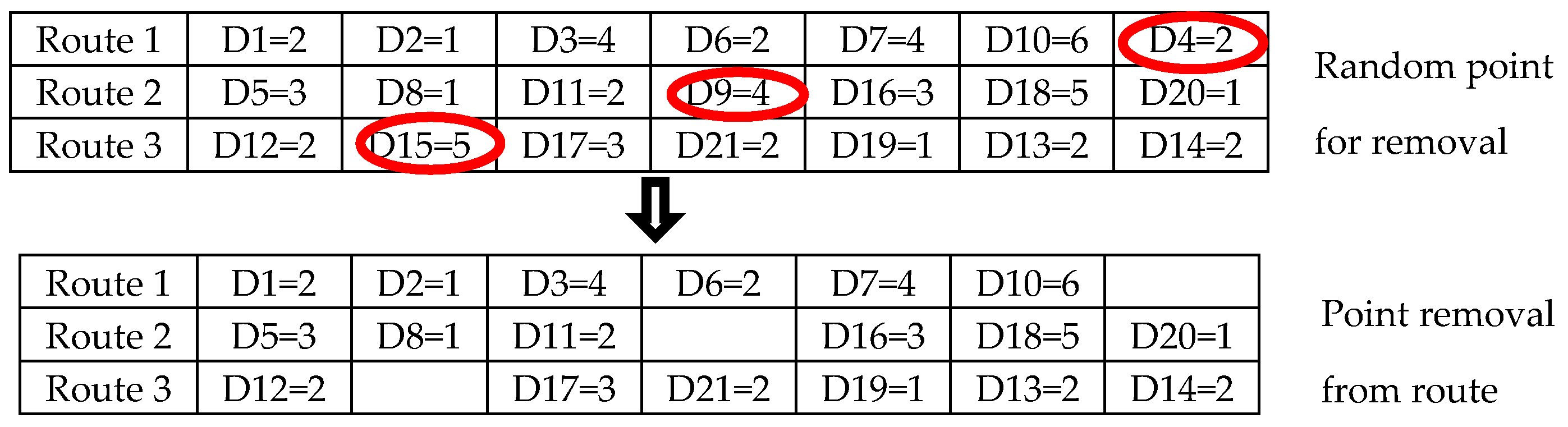
4.2.1. Random Removal

Random removal is a simple method. The q request is selected randomly and is removed from the solution, as shown in Figure 2:

We used two methods of random removal: tourism attraction random removal (TARR) and farm random removal (FRR). These two methods have similar steps:

Step 1

The sort of TARR or FRR is selected randomly for sort destroying.

Step 2

The number of sort destroying is selected randomly for finding the number of point removals.

Step 3

If there is a random number of points, the operation removes the points from the route.

The random point of tourism attraction or farm is removed from the route. After that, the point randomly inserts a new route.

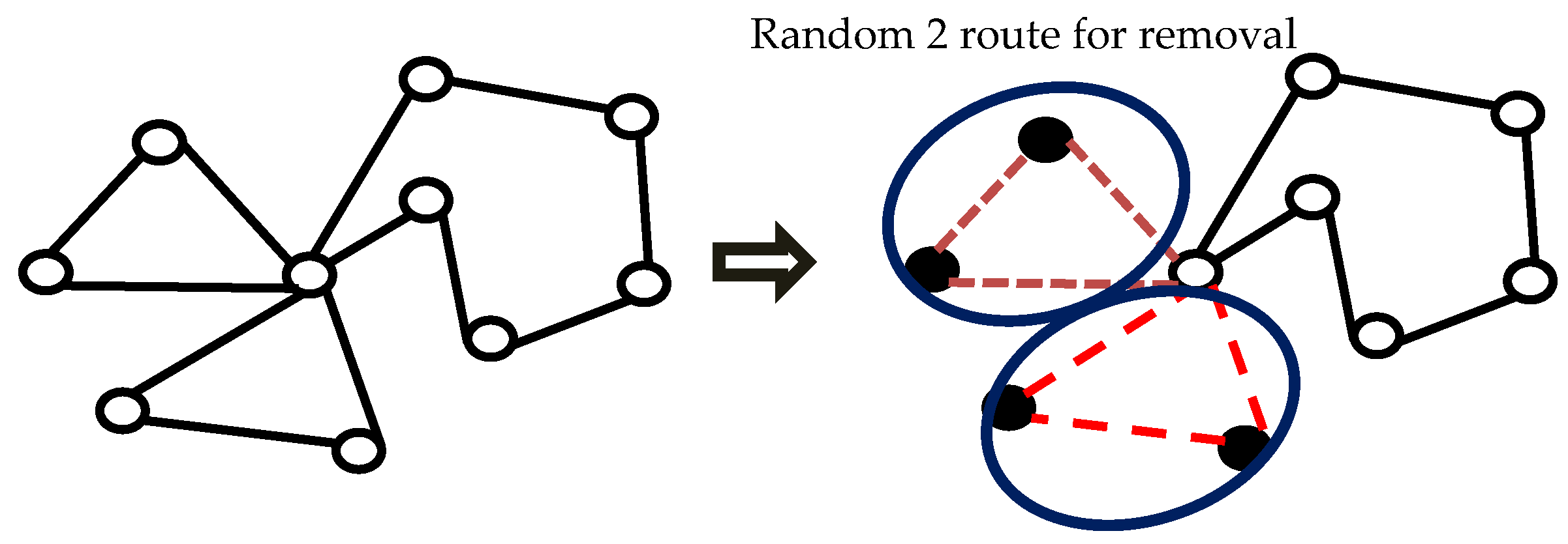
4.2.2. K-Route Removal

Route removal is a destruction operation. We used three removal methods: single route removal (1RR), two-route removal (2RR), and three-route removal (3RR) for destroying the initial solution, as shown in Figure 3. The three removals follow the same K-route removal steps:

Step 1

A route is selected randomly from all the routes; the route randomly selected is one or more from route R $\subseteq$ S |R| = K.

Step 2

Determine A as an array of destination point R.

Step 3

Randomly select the removal method from all route removals.

Step 4

The route is selected from Step 1 is destroyed for finding L, where L is solution set to be removed.

The route random of tourism attraction or farm is removed from all routes. After that the point random inserts a new route for finding the solution.

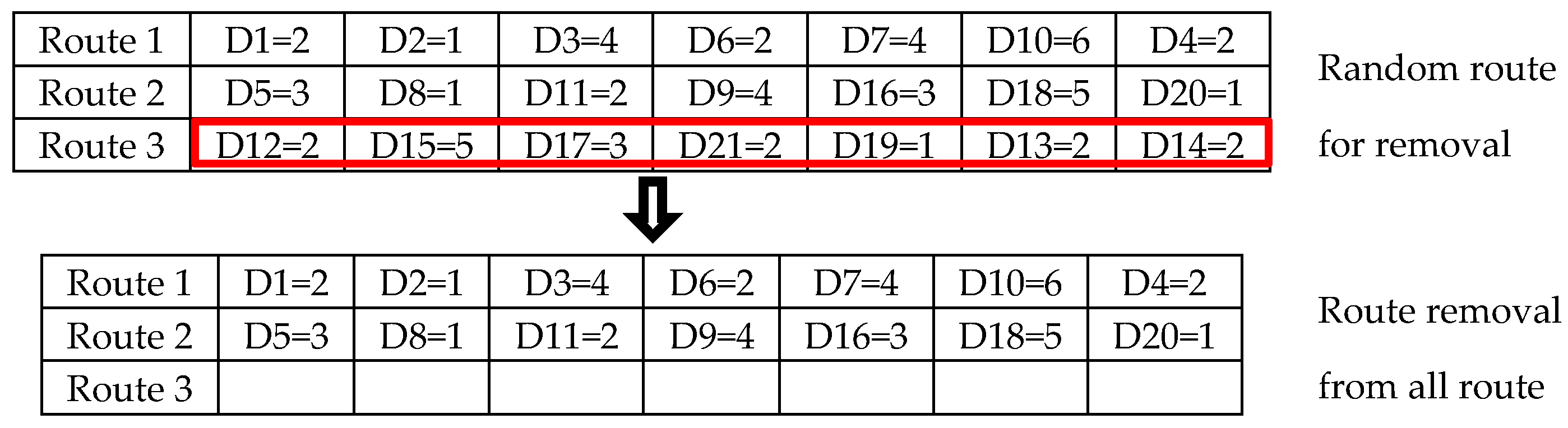
4.2.3. Entire Route Removal

Entire route removal involves destroying the entire traveling route. The route destruction is a route adjustment to find the best solution finding, as shown in Figure 4.

Entire route removal is performed as follows:

Step 1

A route is selected randomly from all the routes, where route random selection is one or more than route R $\subseteq$ S |R| ≥ 1.

Step 2

Determine if A is an array of destination point R.

Step 3

Route was selected for removal from all routes.

Step 4

A route is selected from Step 1 is destroyed for finding L, where L is the solution set to be removed.

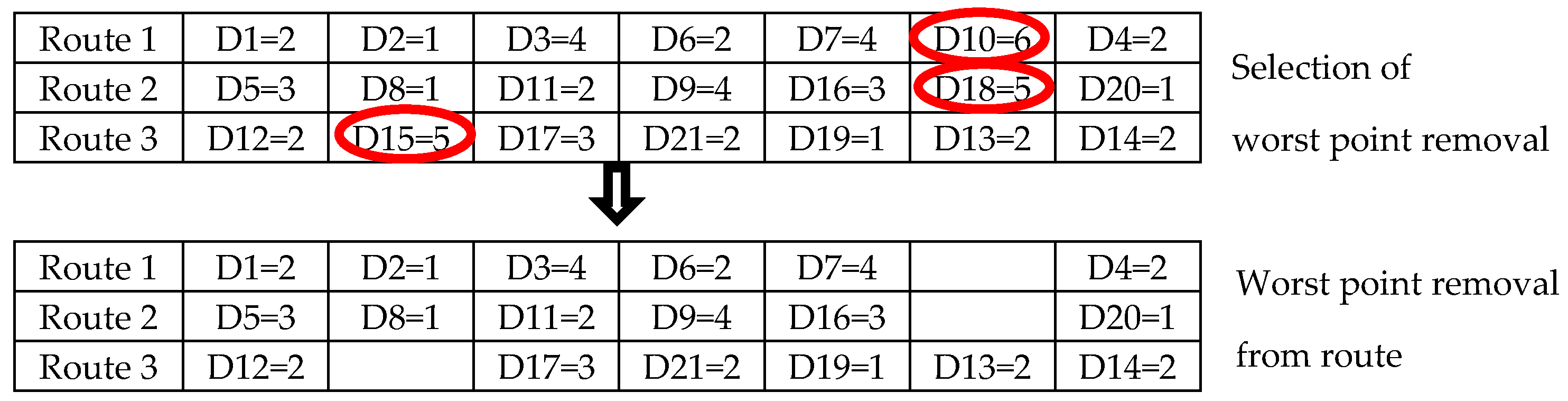
4.2.4. Worst Removal

Worst removal involves removed the worst value for solution improvement. The removal of a tourism attraction or farm was considered using the highest-cost current solution, which was a sorted solution using the cost, shown in Figure 5. The solution involved selected the removal and calculating the new cost, so that solution involved repeating the procedure. In this work, the worst removal involved two removals: the tourism attraction worst removal (WTAR) and the farm worst removal (WFR). The WTAR and WFR have similar step of removal. The algorithm for the two methods is shown in Algorithm 3.

Algorithm 3: Worst removal algorithm.

1. L ← {};

2. While |L| < q do

2.1 Array: A = an array containing all tourism attractions or farms request from s not in L;

2.2 Sort A such that (i < j) → cost(A[i]) < cost(A[j]);

2.3 Choose a random number x from the interval(0,1);

2.4 L ← L $\cup$ {A[xp |A|]};

3. remove the requests in L from s;

4. return L

The four steps of worst removal are:

Step 1

The initiation is a vacant set.

Step 2

Find L by repeating this procedure completely for the number of q:

2.1

Array A is a created number of all tourism attractions or farms but set L is untraceable.

2.2

Array A member is sorted by using cost function removal.

2.3

Random x is an interval in the range 0–1.

2.4

A tourism attraction or farm is a selected value in array A, in which an attraction point is random. Then, add a tourism attraction point or farm point to the set of L, where the value p is a random weight. A low value of p corresponds to greater randomness.

Step 3

The member completely removes point L from the solution.

Step 4

Return L is Step 2, where L is found in the next iteration.

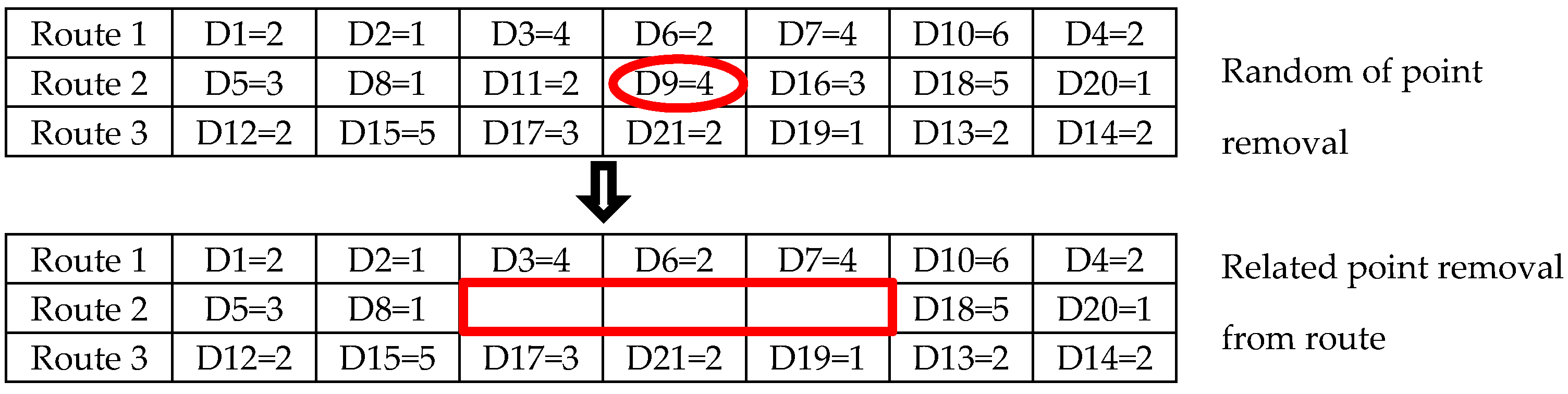
4.2.5. Related Removal

We used related removal, which is a destruction operation based on Shaw (1997). Related removal includes two removal methods: tourism-attraction-related removal (TAREL) and farm-related removal (FREL). The tourism route and farm route are randomly selected for removal from all nodes in the solution, as shown in Figure 6. The TAREL and FREL algorithms follow similar steps as shown in Algorithm 4.

Algorithm 4: Related removal algorithm.

1. L ← {};

2. Random centroids p(lat,lng)

3. While |L| < q, then

3.1 Find ct is a nearly centroid tourism attraction point or farm point with Euclidean distance

3.2 L ← L $\cup$ {ct};

3.3 Update centroids p(lat,lng) = centroids(L) = $\frac{{\displaystyle \sum _{\mathrm{i}}^{\left|\mathrm{L}\right|}\mathrm{L}\left[\mathrm{i}\right]}}{\left|\mathrm{L}\right|}\mathrm{lat},\frac{{\displaystyle \sum _{\mathrm{i}}^{\left|\mathrm{L}\right|}\mathrm{L}\left[\mathrm{i}\right]}}{\left|\mathrm{L}\right|}\mathrm{lng}$;

4. return L

The five steps of related removal are:

Step 1

A single tourism attraction position or single farm position is selected randomly from all the tourism attractions or farm locations, respectively, which is removed from the solution.

Step 2

The generated group set removal is an initial member c_t.

Step 3

Finding L involves a repeated procedure for the number of q.

3.1

One tourism attraction position or farm position is chosen at random from the set of L.

3.2

Array A is a created member of all solutions but untraceable from set L.

3.3

Array A member is sorted by using the function relation R(c₁,c₂) from less to more valuable. The defined relationship is a distance between c₁ and c₂ plus the opening time of destination c₁,c₂ finding from R(c₁,c₂) = α dist(c₁,c₂) + β|tac₁ − tac₂|.

3.4

Random x is an interval ranging from 0–1.

3.5

A point of tourism attraction or farm is a selected value in array A, of which the tourism attraction point or farm point is a random value. After that, the tourism attraction point or farm point is added to set L, where the value p is of random weight random, and a low value of p corresponds to greater randomness.

Step 4

When the member is completely removed, point L is the solution.

Step 5

Return L is Step 2, where L is found in the next iteration.

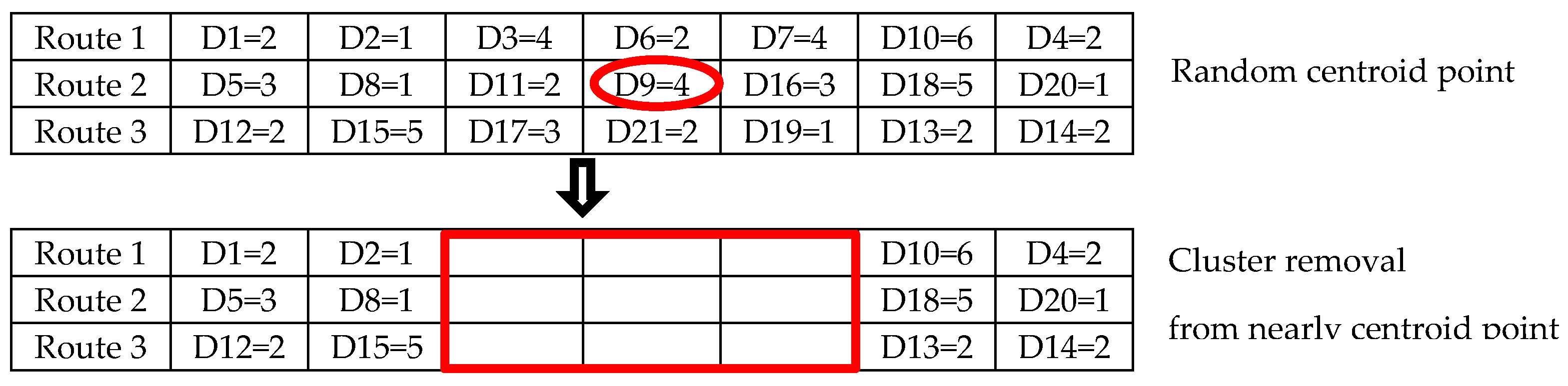
4.2.6. Cluster Removal

Cluster removal is a destruction method for a random route for finding the centroid in a solution. Then, the Euclidean distance method is used for finding an attraction point near the centroid, and this point is an improvement on the centroid position, aa shown in Figure 7.

The cluster removal method includes tourism attraction cluster removal (TACR) and farm cluster removal (FCR). The algorithm of cluster removal is shown in Algorithm 5.

Algorithm 5: Cluster removal algorithm.

1. Randomly select a tourism attraction or farm ct and remove it from the solution;

2. L ← {ct};

3. while |L| < q then

3.1 c ← randomly select a travel place in L;

3.2 Array: A = an array containing all request from s not in L;

3.3 Sort A such that (i < j) → R(c,A[i]) < R(c,A[j]);

3.4 Choose a random number x from the interval [0,1);

3.5 L ← L $\cup$ {A[xp |A|]};

4. remove the requests in L from s;

5. return L

The cluster removal steps are as follows:

Step 1

The initiation is a vacant set.

Step 2

Randomly choose centroids for removal.

Step 3

Finding L was repeated for the number of q.

3.1

Find point c_t as a nearly centroid point using the Euclidian distance method.

3.2

A point is added in set L.

3.3

The updated centroid is an improvement in the solution route.

Step 4

Remove L from solution S.

Step 5

Return L is Step 2 that found L in the next iteration.

The tourism attraction or farm removed random is nearly centroid of all routes. After that, a point is randomly inserted as a new route for solution finding.

4.3. Repairing Operation

When a destruction operator is applied, then a repairing operation is used to improve the solution. We used five different repairing operations.

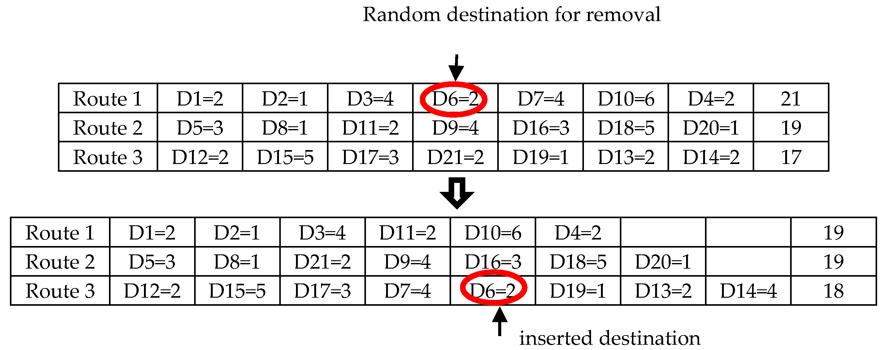
4.3.1. Greedy Insertion

Greedy insertion is a repairing of solutions used for finding the differences in the lowest cost before the reinsertion solution is applied to a route for anew solution. An example of greedy insertion is shown in Figure 8.

The steps for greedy insertion are as follows:

Step 1

Determine S as a solution set member {r₁, r₂, ..., r_k}.

Step 2

Repeat each r_k $\in$ S to find the difference in the lowest cost with insertion c into i of r_k Δf_c,k.

Step 3

The destination position is inserted into different lowest-cost routes of all routes, as shown in Equation (37):

$$\mathrm{c}=\mathrm{m}\mathrm{i}{\mathrm{n}}_{\mathrm{c}\in \mathrm{L}}\Delta {\mathrm{f}}_{\mathrm{c},\mathrm{k}}$$

(37)

where c is the lowest cost, L is all positions not free, k is the destination number, and f is the different lowest value of the route.

4.3.2. Regret-H Insertion

Regret-H insertion provides a forward data view, which has been used to improve the behavior of greedy insertion heuristic (Ropke and Pisinger 2006; Potvin and Rousseau 1993). The Regret-H insertion is shown in Figure 9.

The regret insertion used in this study determines x_c,h $\in$ {1, 2, …, H} for insertion into the solution as shown in Equation (38):

$${\mathrm{c}}^{\prime }={\max }_{\mathrm{c}\in \mathrm{L}}\left\{{\displaystyle \sum _{\mathrm{h}=1}^{\mathrm{H}}(\Delta {\mathrm{f}}_{\mathrm{c},{\mathrm{x}}_{\mathrm{c},\mathrm{h}}}-\Delta {\mathrm{f}}_{\mathrm{c},{\mathrm{x}}_{\mathrm{c},1}})}\right\}$$

(38)

where x_c,h is the point of insertion for destination point c and is a sequential insertion to h. The destination shows the highest value of sequence H-regret insertion, which is inserted at the position of lowest cost.

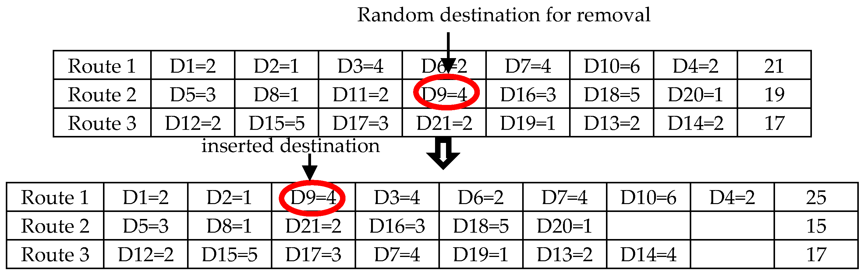
4.3.3. Greedy Insertion with New Route Opening

This insertion improves upon greedy insertion by opening a new route. It operates based on the greedy insertion for the best solution. The greedy insertion with new route opening is described as follows:

Step 1

Total number of routes is determined as the highest number of routes.

Step 2

When the number of routes is less than the prescribed route:

2.1

If the creative new route is less expensive than the cost of greedy insertion, the new route is created.

2.2

Vise versa: if the creative new route is not better than the cost of greedy insertion, the greedy insertion is selected for insertion.

Step 3

If the new route is over prescribed, the greedy insertion is selected instead of a new route.

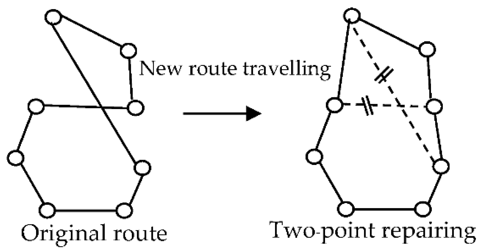
4.3.4. Two-Option Route Repairing

Two-option route repairing is a practical local search for the solution that repairs the excess effective new solution. Two-option route repairing follows the new routing pattern with random removal of routes traveling between two tourism attractions. Then, the route is sorted by a link with a new route. Two-opt route repairing is shown in Figure 10. The new solution created by two-opt route repairing is shorter than the old solution, creating a more effective solution.

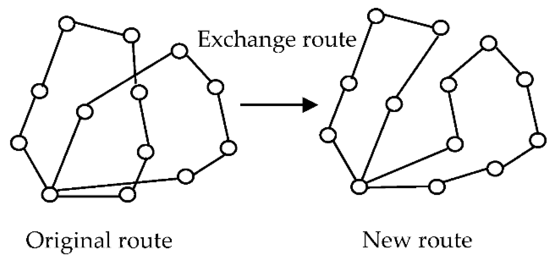
4.3.5. Exchange Route Repairing

Exchange route repairing is a local search for an improved solution in the repairing operation. The traveling route is exchanged with a selected randomly removed traveling route point on each route. After that, the traveling route point removal creates a new route to improve the solution. The exchange route repairing method is shown in Figure 11. The new routes have a shorter traveling distance, which is the best solution.

4.4. Acceptance Criterion

The simulated annealing method has been used for accepting or rejecting a new solution (Kirkpatrick et al. 1990). The new solution s′ is accepted over the current solution s when new solution s′ is better than current solution s. The new solution is accepted with probability shown in Equation (39):

$${\mathrm{e}}^{\frac{-(\mathrm{f}({\mathrm{s}}^{\prime })-\mathrm{f}(\mathrm{s}))}{\mathrm{t}}}$$

(39)

where t is the temperature parameter and f is the objective function. In this study, we minimized this problem, which was obtained by the total distance between the attraction and the farm in each route. The simulated annealing method begins with some initial temperature values when the value is lowered from emphasis to value cumulative with setting T ← C·T. Therefore, the moderate value of T was accepted considering the non-improved solution from the probability.

5. Results and Discussion

The Lingo program and ALNS algorithm were run on a computer with Intel® Core™ i5-2320M CPU @ 3.00 GHz with 4 GB RAM Memory under the Windows operating system. The parameter input for each problem size was similar for both Lingo and the ALNS algorithm. The results from the Lingo program and the ALNS algorithm were compared for three problem sizes: small, medium, and large. The small problem included 10 tourism attractions and 5 farms, the medium-sized problem included 40 tourism attractions and 15 farms, and the large included 80 attractions and the 25 farms. Each problem size was tested with five instances. From the comparison of the results, the ALNS algorithm was able to solve the tourism route and facilities location problems to support tourists for all problem sizes. The results from the Lingo program and the ALNS algorithm are shown in

Table 2. The result comparison of Lingo program and the ALNS algorithm.

Problem Size	No.	Parameter		Lingo Program			ALNS		Difference
				Result			Result
		i, j	f	Status	Total Distance (km)	Processing Time (h)	Total Distance (km)	Processing Time (h)	Total Distance (km)	Processing Time (h)	Gap in Distance Traveled (%)	Processing Time Gap (%)
Small	S-1	10	5	Global Opt	109.90	00:00:01	109.90	00:00:01	0	0	0.0	0.0
	S-2	10	5	Global Opt	164.40	00:00:01	164.40	00:00:01	0	0	0.0	0.0
	S-3	10	5	Global Opt	302.60	00:00:33	302.60	00:00:33	0	0	0.0	0.0
	S-4	10	5	Global Opt	308.73	00:00:58	308.73	00:00:58	0	0	0.0	0.0
	S-5	10	5	Global Opt	286.60	00:00:37	286.60	00:00:37	0	0	0.0	0.0
Average					234.45	00:00:24	234.45	00:00:24	234.45	0	0.0	0.0
Medium	M-1	40	15	Feasible	898.65	40:59:27	901.50	00:05:05	−2.85	40:54:22	−0.32	99.88
	M-2	40	15	Feasible	1157.84	60:17:21	1161.01	00:05:05	−3.17	60:12:16	−0.27	99.92
	M-3	40	15	Feasible	997.78	41:49:13	1002.37	00:05:55	−4.59	41:43:46	−0.46	99.88
	M-4	40	15	Feasible	1131.47	55:56:29	1153.50	00:05:25	−22.03	55:51:02	−1.95	99.91
	M-5	40	15	Feasible	992.78	50:49:25	1018.52	00:05:45	−25.74	50:44:20	−2.59	99.90
Average					1035.70	49:45:24	1047.38	00:05:25	−11.68	49:40:28	−1.12	99.90
Large	L-1	80	25	Lower bound	2058.56	>120	2077.58	00:14:48	−19.02	119:51:52	−0.92	99.88
	L-2	80	25	Lower bound	1938.81	>120	1987.10	00:13:46	−48.29	119:50:54	−2.49	99.89
	L-3	80	25	Lower bound	2076.52	>120	2099.13	00:15:54	−22.61	119:51:46	−1.09	99.87
	L-4	80	25	Lower bound	1965.64	>120	1973.07	00:14:51	−7.43	119:50:49	−0.38	99.88
	L-5	80	25	Lower bound	2087.31	>120	2092.70	00:15:43	−5.39	119:50:57	−0.26	99.87
Average					2025.37	120	2045.92	00:14:54	−20.55	119:50:48	−1.03	99.88

Note: i, j are tourism attractions at position i, j and f is farm number.

. The ALNS algorithm was able to quickly solve the problem for various numbers of visited tourism attractions. The ALNS algorithm result was not different from that produced by Lingo, which provided a highly effective solution for tourism route planning and the selection of suitable shopping outlet locations.

The balance of tourism attractions and minimum traveling distance was attained using the random destruction and repair methods with the addition of the ALNS approach. From the computational results for all problem sizes, we found that the five small problem case studies showed a global optimal result (total distance and processing time) that was not different from the result produced by Lingo. In conclusion, the ALNS algorithm and the Lingo program produced the same results for all small problems because the small problems are easy to solve quickly. These cases involved fewer tourism attractions and farms. As a result, the problems were not complex. The optimal feasible solution for all small problems was an average total distance traveled of 234.45 km. There was no gap between the results produced by the Lingo program and ALNS algorithm, which used the destruction and repairing of ALNS to accurately analyze the input data. Therefore, the ALNS algorithm was effectively equal to the Lingo program for this type of problem.

For all medium-sized problems, the ALNS algorithm produced a different total traveling distance result compared with the Lingo program. However, the Lingo program required a longer processing time than ALNS. The average processing time was 49.45 h for the Lingo program, which is a long processing time, as the problem is only analyzed for a global solution. Therefore, the Lingo program requires long processing times whenever the numbers of destinations and farms increase, creating a complex problem. The processing time required for the ALNS algorithm was shorter. The ALNS provides a specific feasible solution; as a result, the processing time was shorter. The average ALNS processing time was 5.25 min.

For the large problem, the Lingo program was unable to provide a global or feasible solution, due to the complexity of the problem due to the large number of incorporated tourism attractions. The Lingo program required over 120 h of processing time. However, the Lingo program produced a result with a lower bound, which was used for a comparison with ALNS. The total travel distance produced by the Lingo program was slightly shorter than that produced by ALNS. The ALNS algorithm provided effective problem solving with a fast processing time. The ALNS algorithm required about 15 min of processing time. Although the results produced by the ALNS algorithm are not the global optimal solution, the solution can be considered acceptable. An effective computation comparison of the Lingo program and the ALNS algorithm demonstrated the similarity in the average total traveling distance. However, the Lingo program provides a shorter total traveling distance compared to that provided by the ALNS algorithm. However, the ALNS processing time for medium- and large-sized problems was much lower in comparison to that of the Lingo program.

The comparison of the results provided for each problem is provided in Table 2. From the differences in the results seen in Table 2, the average total traveling distance produced by ALNS is different from the Lingo program for the medium-sized and large-sized problems. There was no observed difference in the results for the small problem. The average total traveling distance results obtained by the Lingo program were shorter compared to those obtained by ALNS, by 11.68 km shorter for all medium-sized problems and 20.55 km for large-sized problems, which is, on average, 1.12% shorter of the medium-sized problems and 1.03% shorter for the large-sized problem. However, many previously-introduced algorithms were reported to have a gap between 0.04 and 15% from the Lingo program, which is an acceptable result from a research point of view. Therefore, the small difference between the two methods in terms of the total traveling distance for the medium- and large-sized problems is considered an acceptable result.

The ALNS has many destruction and repair methods that were randomized for finding the best solution in each computational round and testing the solution until the optimal feasible was found. Both medium- and large-sized problems are receiving increasing research attraction due to the complexity of data analysis in an optimal solution-finding problem-solving process. The randomness of both the destroying and repair methods that differ in each computational round cause the solution to always be exchanged during solution computation. Therefore, the gaps in the solutions provided by the ALNS algorithm and the Lingo program for both the medium and large problems were different.

From the comparison of the Lingo program and the ALNS algorithm, there was no difference in the average processing time for the small problem, but a difference was observed in the average processing time of the ALNS algorithm for the medium and large problems. The Lingo program required 49.40 h and 119.50 h of computation for the medium and large problems, respectively. The ALNS algorithm was able to effectively reduce the computation time by 99.9% and 99.8% for the medium and large problems, respectively. The ALNS algorithm rapidly provided a highly effective solution for a complex problem. The results produced by the Lingo program and ALNS algorithm are provided in Table 2. The results were analyzed using statistical methods for performance comparison. The total traveling distance result of all problem sizes are tested normality with a significant level of 0.05, as shown in

Table A4. Normality testing of data provided in Table 1.

Normality Testing	Problem Size
	Small		Medium		Large
	Lingo	ALNS	Lingo	ALNS	Lingo	ALNS
p-value	0.119	0.119	0.419	0.388	0.430	0.100
Results	normal	normal	normal	normal	normal	normal

. All the p-values were significant, with values smaller than 0.05. Therefore, the data for all problem sizes were normally distributed. Afterward, the data for all problem sizes were tested for the average difference using statistical methods. We used a paired T-test with a significance level 0.05, and the results are shown in

Table 3. Results of paired t-test from data in Table 1.

Problem Size	p-Value
	Total Traveling Distance	Processing Time
Small	1.000	1.000
Medium	0.081	0.000 *
Large	0.055	0.000 *

Note: * significant difference of method.

.

From the above table, the statistics show a significant p-value beyond the 0.05 level for the total traveling distance for all problem sizes. The difference between the Lingo program and the ALNS algorithm was not significant. The processing time for the small problem had a p-value higher than the 0.05 level, denoting no significant difference between the two methods. However, the processing times for the medium and large problems had p-values lower than the significant level, demonstrating the difference between Lingo and ALNS. Therefore, the ALNS algorithm reduces the processing time for problem solving, while producing a total traveling distance that is not different from result provided by Lingo. The ALNS algorithm is a suitable and highly effective method for solving complex vehicle routing problems involving many destinations.

6. Conclusions

In this study, we examined a tourism route design problem and attempted to determine the appropriate location for tourism facilities in Thailand. The ALNS algorithm method was used to solve the vehicle routing problem to help design an appropriate travel route and to choose the best location for tourism facilities. The traveling distance results produced by the ALNS algorithm were similar to those produced by the Lingo program for all problem sizes. However, for high numbers of tourism attractions and farms (complex problem), the ALNS algorithm required significantly less processing time than the Lingo program, effectively reducing the computation time by 99.8% for the medium problem and 99.7% for the large problem. For all problems, the total traveling distance results produced by the two methods were not significantly different. Therefore, ALNS is a suitable method for designing tourism routes, rapidly providing highly effective solutions for complex problems with a large number of attractions.

Case Study

A tourism route was designed using the ALNS method for a case study. To create a large and complex problem, 115 tourism attractions and 25 farms were used in this case study, as shown in Table A1 and Table A2. The result of the case study is provided in

Table 4. Case study result.

Problem	Route	Destinations	Outlet Locations	Farms	Distance (km)	Distant Total (km)
Case study	1	0-7-15-9-21-0	9	4,1	55.60	2538.02
	2	0-81-71-72-77-75-74-91-94-80-3-0	71	11	279.40
	3	0-8-28-29-83-103-114-115-113-76-73-79-82-0	114	22,10	379.80
	4	0-49-50-52-51-48-106-68-66-0	106	16,14	171.95
	5	0-1-27-14-18-0	1	2,6,7,5	119.63
	6	0-67-102-99-105-111-112-100-109-107-108-101-104-110-70-32-0	108	13,15	202.79
	7	0-11-45-42-41-2-23-0	41	21	209.70
	8	0-16-44-46-47-43-88-90-87-85-84-86-89-40-0	47	20,18	337.50
	9	0-25-26-22-60-61-58-62-59-69-64-20-0	20	19,3	184.40
	10	0-19-95-93-96-97-98-92-78-30-4-0	92	17,9	234.60
	11	0-10-31-5-37-34-35-36-39-38-33-24-0	34	25,24,23	201.85
	12	0-63-65-55-57-54-56-53-0	54	8	133.40
	13	0-13-17-12-6-0	12	12	27.40

.

The algorithm designed 13 different traveling routes for the case study. Each tourism route in the case study was limited to 11 h of travel in one day. Accordingly, the first travel route involves sightseeing on the first day. For example, the order for tourism attraction sightseeing is 0-7-15-9-21-0 for route 1, where 0 is the hotel or home base, and destination 9 is a shopping outlet. The order of farm product transportation is the first farm and the fourth farm bringing sales products to the ninth destination. The distance traveled for the first route is 55.60 km, and popular and less popular tourism attractions are balanced. The travel distance is minimized for each route. However, the total distance for the case study is 2538.02 km, which is the shortest distance for all traveling routes. The shopping market for all routes is the location where products are sold. The shopping market location is placed in the middle point of each route, occurring between 11:00 a.m. and 2:00 p.m. to allow tourists to take a break and eat. From Table 4, the traveling route for the case study is as shown in Figure 12.

In this case study, the average traveling cost of each route of 2.35 baht/km was calculated using route management. Each route cost is provided in

Table A5. Tourism traveling cost.

Cost Per Unit (Bath/km)	Route	Distance (km)	Traveling Cost (Bath)
2.35	1	55.60	130.66
	2	279.40	656.59
	3	379.80	892.53
	4	171.95	404.08
	5	119.63	281.13
	6	202.79	476.55
	7	209.70	492.79
	8	337.50	793.12
	9	184.40	433.34
	10	234.60	551.31
	11	201.85	474.34
	12	133.40	313.49
	13	27.40	64.39
Total		2538.02	5964.34

. The traveling distance of the third route was highest, with a route distance of 379.80 km and highest traveling cost of 892.53 baht. The 13th route was the shortest, at 27.40 km, with the lowest traveling cost of 64.39 baht. The total traveling cost of tourism in this case study was 5964.34 baht. Therefore, the tourist can choose the best route based on sightseeing and the cost of the tour. This algorithm provides tourism route management with an approach for tourism organization, planning, and support for decision-making.

The empirical results provided by the ALNS algorithm are useful to tourists. Tourists can use the data to help choose which sightseeing attractions to visit and shopping areas for relaxation. The ALNS algorithm can assist with organizing the tourism in Chiang Rai, Thailand by helping to provide route planning and guideline data for tourism public relations. However, the algorithm provided in this study assists with tourism route design while balancing tourism popularity within stated time constraints. There are some constraints that were not included in this work, such as topography, seasonality, and environmental differences. These constraints can be studied using real information to supportable tourism in the future. In future research, different destruction and repair methods will be studied with an effective comparison of each destruction and repair method. Finally, local search algorithms could be applied to the ALNS algorithm to improve the solution. This method can efficiently solve complex problems.

References

1. Alfredo, Olivera, and Viera Omar. 2007. Adaptive memory programming for the vehicle routing problem with multiple trips. Computers & Operations Research 34: 28–47. [Google Scholar] [CrossRef]
2. Alinaghian, Mahdi, and Nadia Shokouhi. 2018. Multi-depot multi-compartment vehicle routing problem, solved by a hybrid adaptive large neighborhood search. Omega 76: 85–99. [Google Scholar] [CrossRef]
3. Andrades, Lidia, and Frederic Dimanche. 2017. Destination competitiveness and tourism development in Russia:Issues and challenges. Tourism Management 62: 360–76. [Google Scholar] [CrossRef]
4. Azi, Nabila, Michel Gendreau, and Jean-Yves Potvin. 2014. An adaptive large neighborhood search for a vehicle routing problem with multiple routes. Computers & Operations Research 41: 167–73. [Google Scholar] [CrossRef]
5. Boonya, Chanagan, and Warisa Wisittipanich. 2017. Mathematical Model for Tourist Routing Problem in a Capital District of Chiang Mai. Paper presented at IE Network 2017, Chiang Mai, Thailand, July 12–15; pp. 1028–33. (In Thai). [Google Scholar]
6. Caroline, Prodhon, and Prins Christian. 2014. A survey of recent research on location-routing problems. European Journal of Operational Research 238: 1–17. [Google Scholar] [CrossRef]
7. Chan, Lu, Eric Hsueh, Shih-Hsin Fang, and Vincent S. Tseng. 2016. Integrating tourist packages and tourist attractions for personalized trip planning based on travel constraints. Geoinformatica 20: 741–63. [Google Scholar] [CrossRef]
8. Chen, Shifeng, Rong Chen, Gai-Ge Wang, Jian Gao, and Arun Kumar Sangaiah. 2018. An adaptive large neighborhood search heuristic for dynamic vehicle routing problems. Computers and Electrical Engineering 67: 596–607. [Google Scholar] [CrossRef]
9. Dayarian, Iman, Teodor Gabriel Crainic, Michel Gendreau, and Welter Rei. 2016. An adaptive large-neighborhood search heuristic for a multi period vehicle routing problem. Transportation Research Part E 95: 95–123. [Google Scholar] [CrossRef]
10. Flognfeldt, Thor, Jr. 2005. The tourist route system—Models of travelling patterns. Belgeo 1: 1–26. [Google Scholar] [CrossRef]
11. Gavalas, Damianos, Charalampos Konstantopoulos, Konstantinos Mastakas, and Grammati Pantziou. 2014. A survey on algorithmic approaches for solving tourist trip design problems. Journal of Heuristics 20: 291–328. [Google Scholar] [CrossRef]
12. Gullhav, Anders N, Jean-Francois Cordeau, Lars Magnus Hvattum, and Bjom Nygreen. 2017. Adaptive large neighborhood search heuristics for multi-tier service deployment problems in clouds. European Journal of Operational Research 259: 829–46. [Google Scholar] [CrossRef]
13. Kang, Eui-Young, Hanil Kim, and Jungwon Cho. 2006. Personalization Method for Tourist Point of Interest (POI) Recommendation. Paper presented at International Conference on Knowledge-Based and Intelligent Information and Engineering Systems KES 2006: Knowledge-Based Intelligent Information and Engineering Systems, Bournemouth, UK, October 9–11; pp. 392–400. [Google Scholar]
14. Kirkpatrick, Scott, C. D. Gelatt, and Mario P. Vecchi. 1990. Optimization by simulated annealing. Science 220: 671–80. [Google Scholar] [CrossRef] [PubMed]
15. Kotiloglu, Serhan, Theodoros Lappas, Konstantinos Pelechrinis, and Panagiotis Repoussis. 2017. Personalized multi-period tour recommendations. Tourism Management 62: 76–88. [Google Scholar] [CrossRef]
16. Liao, Zhixue, and Weimin Zheng. 2018. Using a heuristic algorithm to design a personalized day tour route in a time-dependent stochastic environment. Tourism Management 68: 284–300. [Google Scholar] [CrossRef]
17. Lim, Kwan Hui, Jeffrey Chan, Christopher Leckie, and Shanika Karunasekera. 2018. Personalized trip recommendation for tourists based on user interests, points of interest visit durations and visit recency. Knowledge and Information Systems 54: 375–406. [Google Scholar] [CrossRef]
18. Liu, Long, Jin Xu, Stenhen Shaioy Liao, and Huaping Chen. 2014. A real-time personalized route recommendation system for self-drive tourists based on vehicle to vehicle communication. Expert Systems with Applications 41: 3409–17. [Google Scholar] [CrossRef]
19. Lumsdon, Les, and J. Page Stephen. 2004. Progress in Transport and Tourism Research: Reformulating the Transport-Tourism Interface and Future Research Agendas. In Tourism and Transport. Oxford: Elsevier Science Ltd., pp. 1–27. [Google Scholar] [CrossRef]
20. Nagy, Gabor, and Said Salhi. 2007. Location-routing: Issues, models and methods. European Journal of Operational Research 177: 649–72. [Google Scholar] [CrossRef]
21. Nedjati, Arman, Gokhan Izbirak, and Jamal Arkat. 2017. Bi-objective covering tour location routing problem with replenishment at intermediate depots: Formulation and meta-heuristics. Computers & Industrial Engineering 110: 191–206. [Google Scholar] [CrossRef]
22. Potvin, Jean-Yves, and Jean-Marc Rousseau. 1993. A parallel route building algorithm for the vehicle routing and scheduling problem with time windows. European Journal of Operational Research 66: 331–40. [Google Scholar] [CrossRef]
23. Ram, Yeal, Peter Björk, and Adi Weidenfeld. 2016. Authenticity and place attachment of major visitor attractions. Tourism Management 52: 110–22. [Google Scholar] [CrossRef]
24. Rodríguez, Beatriz, Julian Molina, Fatima Pérez, and Rafael Caballero. 2012. Interactive design of personalised tourism routes. Tourism Management 33: 926–40. [Google Scholar] [CrossRef]
25. Ropke, Stefan, and David Pisinger. 2006. An adaptive large neighborhood search heuristic for the pickup and delivery problem with time windows. Transportation Science 40: 455–72. [Google Scholar] [CrossRef]
26. Shaw, Paul. 1997. A New Local Search Algorithm Providing High Quality Solutions to Vehicle Routing Problems. Glasgow: University of Strathclyde. [Google Scholar]
27. Sirirak, Worapot, Rapeepan Pitakaso, Kanchana Sethanan, and Tassin Srivarapongse. 2018. A Combination of Assignment and Location Routing Problem: A Case Study of Tourism Planning in Chiang Rai Province. Paper presented at 13th International Congress on Logistics and SCM Systems 2018, Ho Chi Minh City, Vietnam, July 29–August 1; pp. 180–84. [Google Scholar]
28. Souffriau, Wouter, and Pieter Vansteenwegen. 2010. Tourist Trip Planning Functionalities: State–of–the–Art and Future. Paper presented at International Conference on Web Engineering, Vienna, Austria, July 5–9; Vienna: Springer, pp. 474–85. [Google Scholar]
29. Vansteenwegen, Pieter, and Dirk Van Oudheusden. 2007. The mobile tourist guide: An OR opportunity. OR Insight 20: 21–27. [Google Scholar] [CrossRef]
30. Wang, Ying-Wei, Chuan-Chih Lin, and Tsung-Ju Lee. 2018. Electric vehicle tour planning. Transportation Research Part D 63: 121–36. [Google Scholar] [CrossRef]
31. Wu, Xiongbin, Hongzhi Guan, Yan Han, and Jiaqi Ma. 2017. A tour route planning model for tourism experience utility maximization. Advances in Mechanical Engineering 9: 1–8. [Google Scholar] [CrossRef]
32. Xiao, Zhou, Li Sen, Fan Yunfei, Liu Bin, Zhang Boyuan, and Li Bang. 2017. Tourism Route Decision Support Based on Neural Net Buffer Analysis. Procedia Computer Science 107: 243–47. [Google Scholar] [CrossRef]
33. Yan, Han, Guan Hongzhi, and Duan Jiaying. 2014. Tour Route Multiobjective Optimization Design Based on the Tourist Satisfaction. Discrete Dynamics in Nature and Society 2014: 603494. [Google Scholar] [CrossRef]
34. Yan, Libo, Bo Wendy Gao, and Meng Zhang. 2017. A mathematical model for tourism potential assessment. Tourism Management 63: 355–65. [Google Scholar] [CrossRef]
35. Yu, Vincent F., Parida Jewpanya, and Anak Agung Ngurah Perwira Redi. 2014. Solving the Multi-Modal Orienteering Problem with Time Windows using Particle Swarm Optimization. Paper presented at Asia Pacific Industrial Engineering & Management Systems Conference 2014, Jeju, Korea, October 12–15. [Google Scholar]
36. Zajac, Sandra. 2017. An Adaptive Large Neighborhood Search for the Periodic Vehicle Routing Problem. In International Conference on Computational Logistics. Southampton: Springer, pp. 34–48. [Google Scholar] [CrossRef]
37. Zheng, Weimin, Xiaoting Huang, and Yuan Li. 2017. Understanding the tourist mobility using GPS: Where is the next place? Tourism Management 59: 267–80. [Google Scholar] [CrossRef]
38. Zhu, Chenbo, J.Q. Hu, Fengchun Wang, Yifan Xu, and Rongzeng Cao. 2012. On the tour planning problem. Annals of Operations Research 192: 67–86. [Google Scholar] [CrossRef]
Figure 1. Problem framework.
Admsci 08 00072 g001
Figure 2. Example of three random removals.
Admsci 08 00072 g002
Figure 3. Example of K-route removal.
Admsci 08 00072 g003
Figure 4. Example of the removal of two entire routes.
Admsci 08 00072 g004
Figure 5. Example of worst point removal.
Admsci 08 00072 g005
Figure 6. Example of related removal.
Admsci 08 00072 g006
Figure 7. Example of cluster removal.
Admsci 08 00072 g007
Figure 8. Example of one randomly constructed solution and greedy insertion.
Admsci 08 00072 g008
Figure 9. Example of one random removal and regret insertion.
Admsci 08 00072 g009
Figure 10. Two-opt route repairing method.
Admsci 08 00072 g010
Figure 11. Exchange route repairing pattern.
Admsci 08 00072 g011
Figure 12. Tourism route design for the case study.
Admsci 08 00072 g012