
A Development of a Robust Machine for Removing Irregular Noise with the Intelligent System of Auto-Encoder for Image Classification of Coastal Waste


Abstract
:
1. Introduction
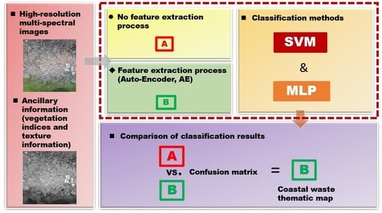
2. Materials and Methods
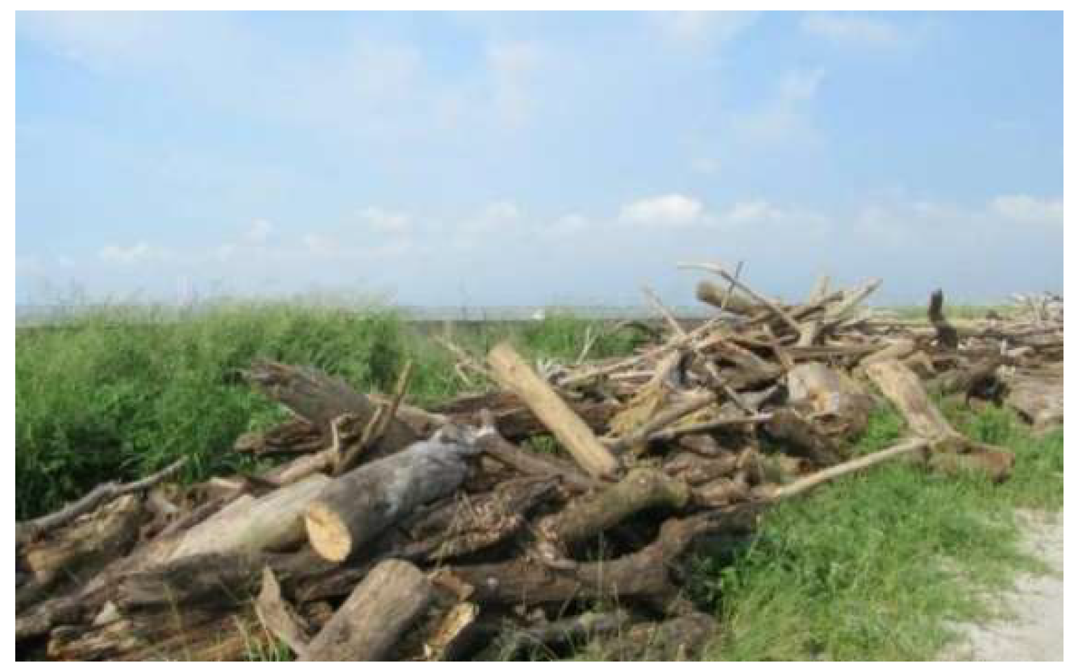
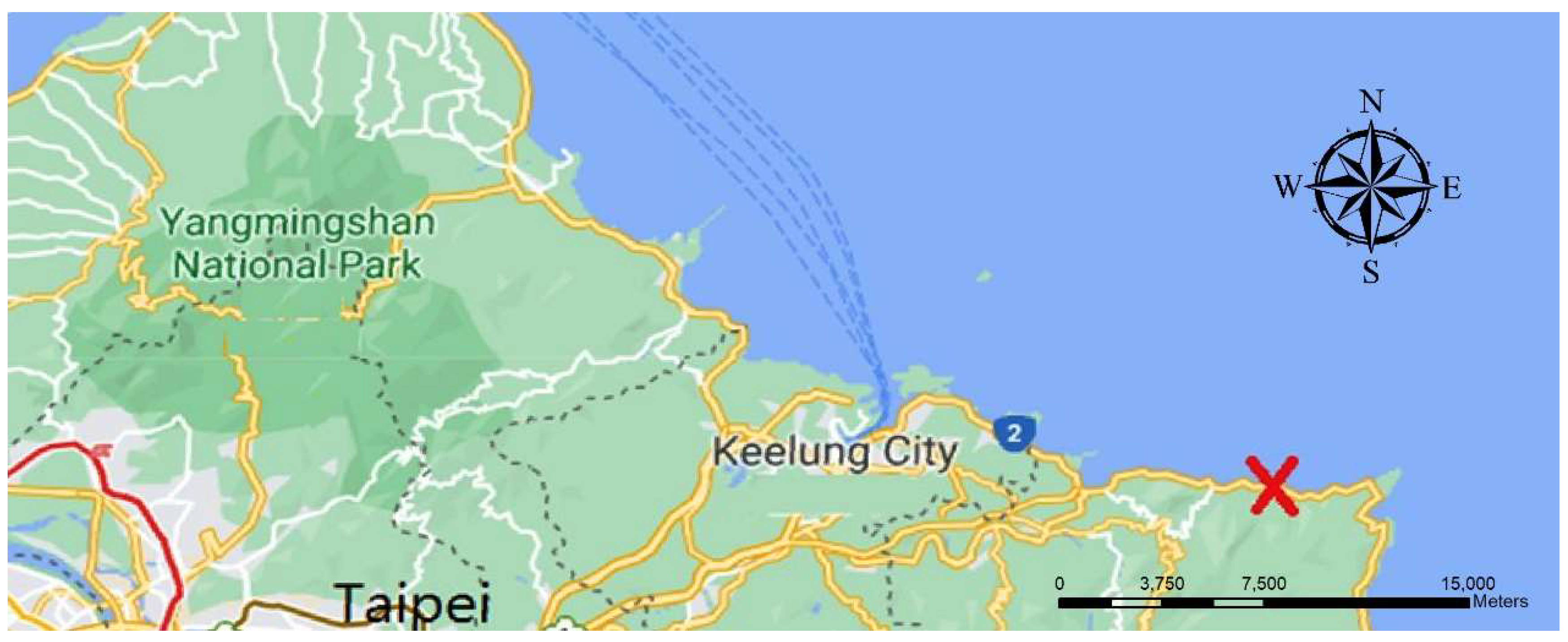
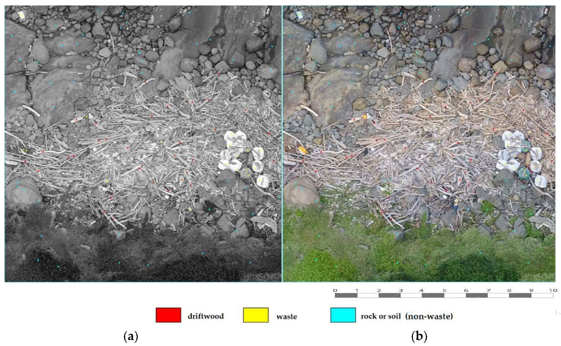
2.1. Study Area
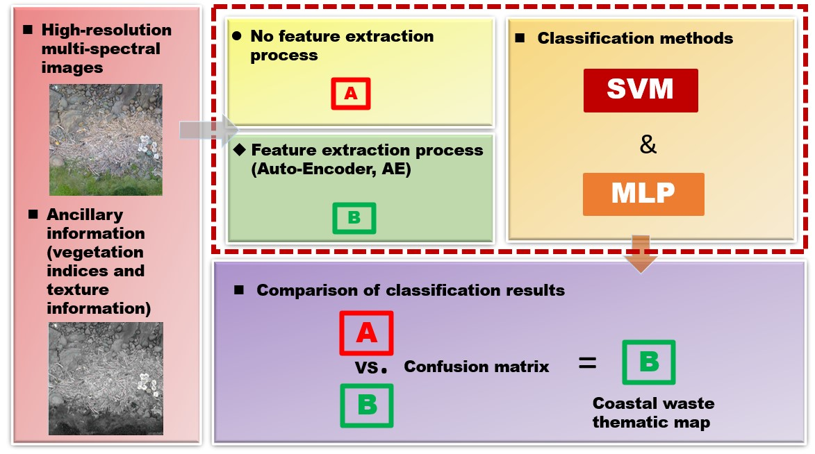
2.2. Image Format
2.3. Ancillary Information
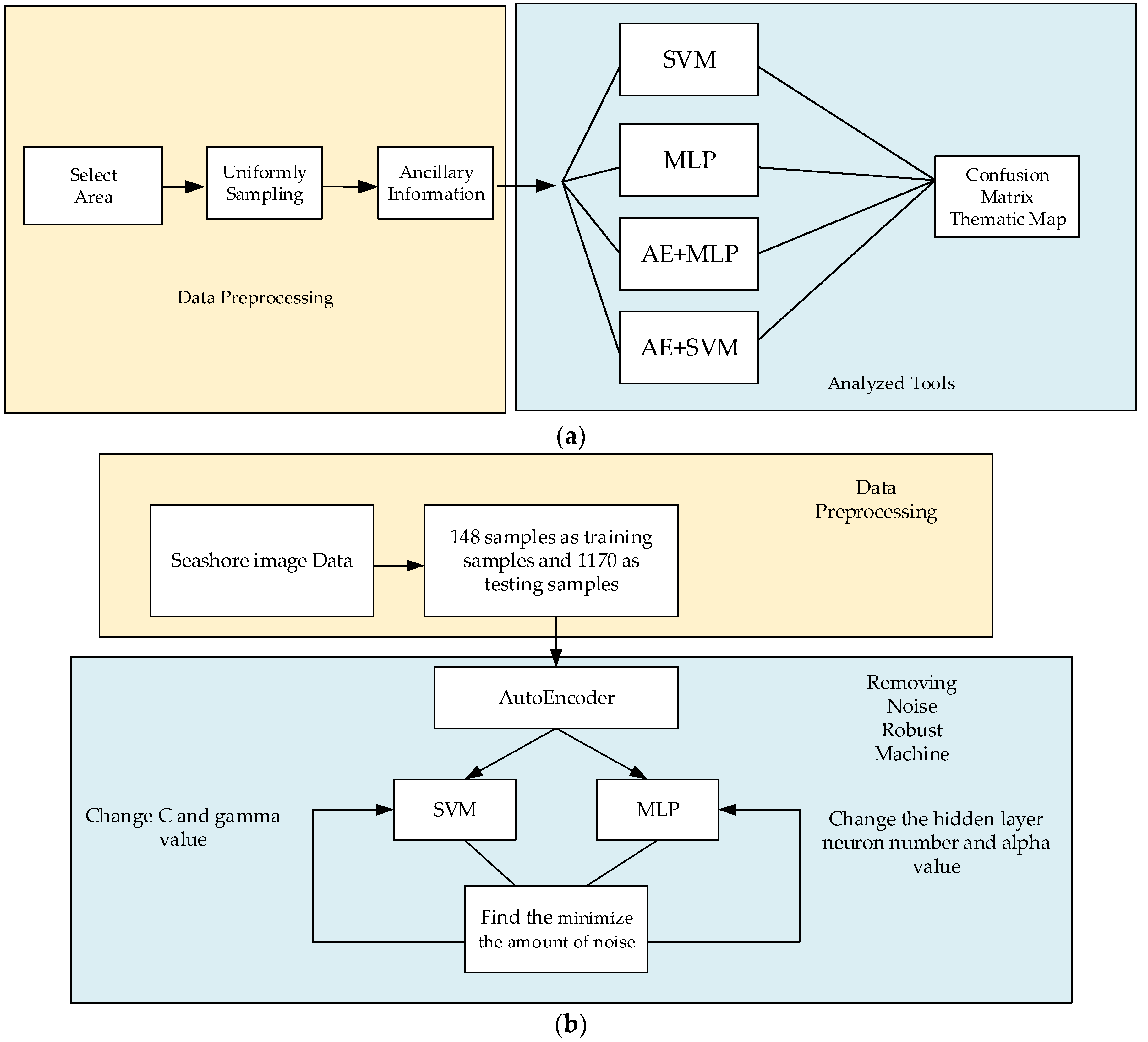
3. Method for Study Plan
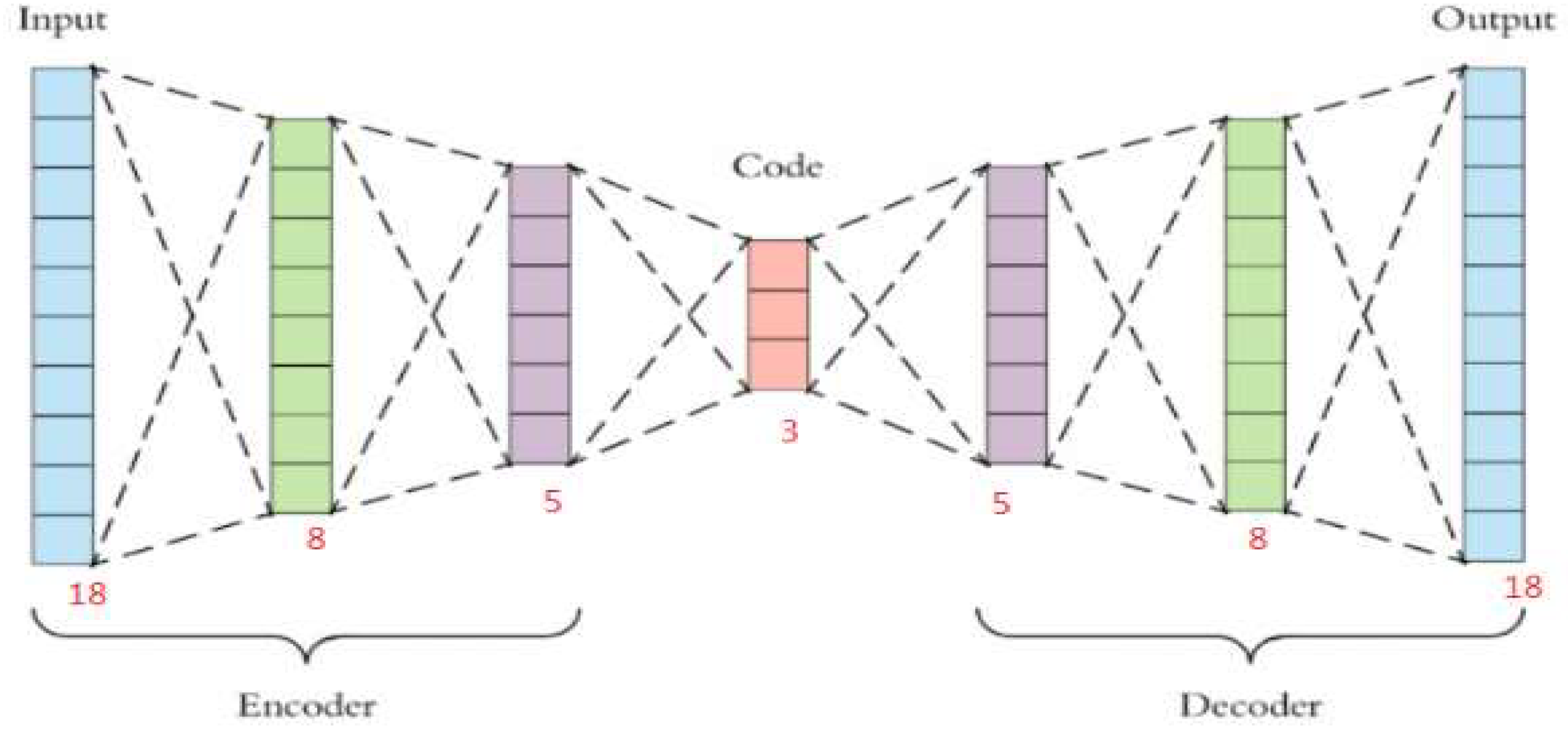
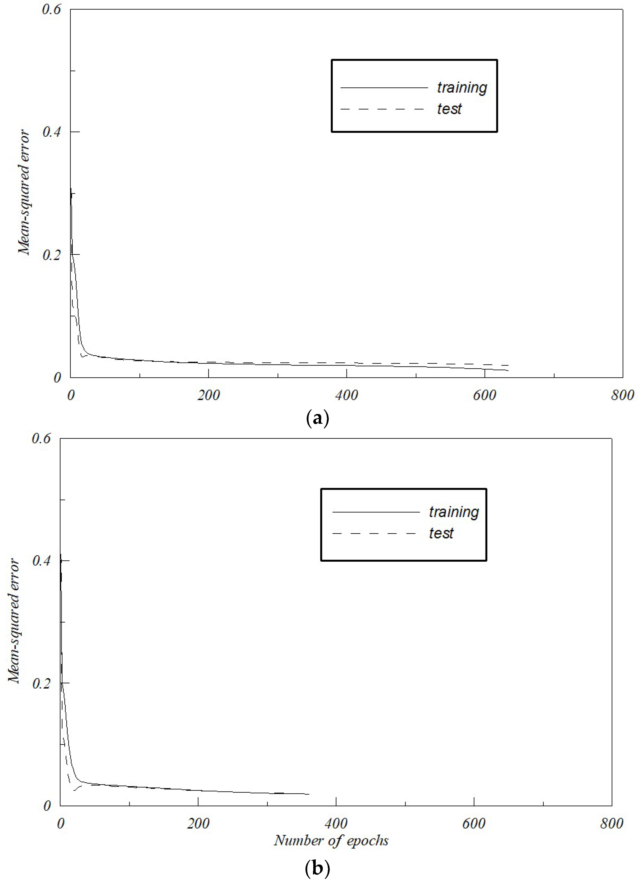
3.1. Auto-Encoder (AE)
3.2. Multi-Layer Perceptron (MLP)
3.3. Support Vector Machine (SVM)
3.4. Development of Robust Removing Noise Machine
4. Results
4.1. Preparing Data for SVM and MLP
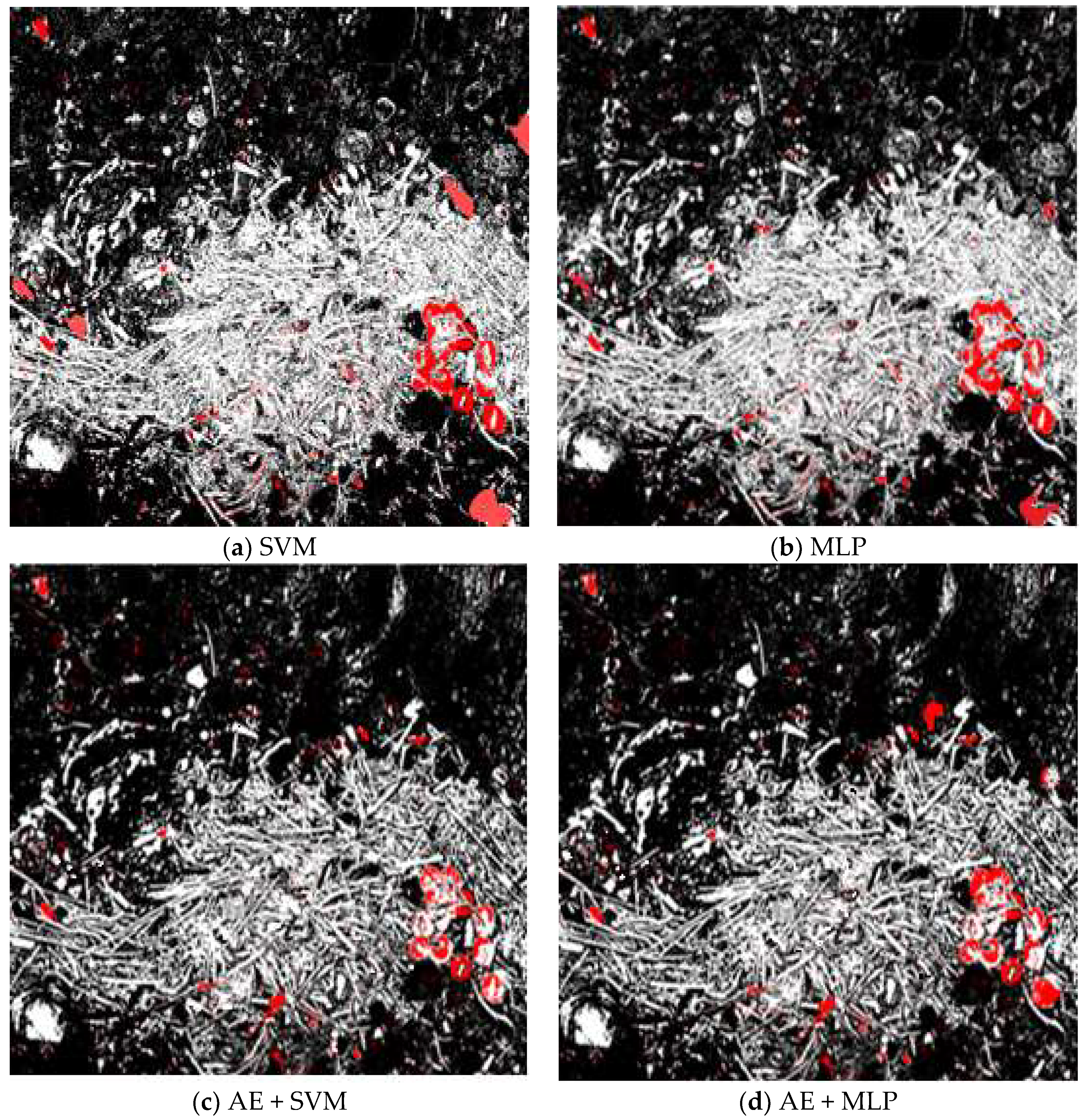
4.2. Thematic Maps
5. Summary and Conclusions
Author Contributions
Funding
Data Availability Statement
Acknowledgments
Conflicts of Interest
References
- Martín, L.; Howarth, P. Change-detection accuracy assessment using SPOT multispectral imagery of the rural-urban fringe. Remote Sens. Environ. 1989, 30, 55–66. [Google Scholar] [CrossRef]
- Turner, M.D.; Congalton, R.G. Classification of multi-temporal SPOT-XS satellite data for mapping rice fields on a West African floodplain. Int. J. Remote Sens. 1998, 19, 21–41. [Google Scholar] [CrossRef]
- Alajlan, N.; Bazi, Y.; Melgani, F.; Yager, R.R. Fusion of supervised and unsupervised learning for improved classification of hyperspectral images. Inf. Sci. 2012, 217, 39–55. [Google Scholar] [CrossRef]
- Lillesand, T.; Kiefer, R.W.; Chipman, J. Remote Sensing and Image Interpretation, 5th ed.; John Wiley & Sons: Hoboken, NJ, USA, 2004; ISBN 0471152277. [Google Scholar]
- Williams, A.T.; Coe, J.M.; Rogers, D.B. Marine Debris: Sources, Impacts and Solutions. Geogr. J. 1999, 165, 233. [Google Scholar] [CrossRef]
- Coe, J.M.; Rogers, D.B. (Eds.) Marine Debris: Sources, Impacts, and Solutions; xxxv, 432p. New York: Springer-Verlag, 1997. Price DM 128.00. J. Mar. Biol. Assoc. UK 1997, 77, 917. [Google Scholar] [CrossRef]
- Calder, D.; Choong, H.; Carlton, J.; Chapman, J.; Miller, J.; Geller, J. Hydroids (Cnidaria: Hydrozoa) from Japanese tsunami marine debris washing ashore in the Northwestern United States. Aquat. Invasions 2014, 9, 425–440. [Google Scholar] [CrossRef]
- Wyles, K.J. The Human Dimension of Marine Litter: The Impacts on Us. Conserv. Biol. 2004. Available online: https://fsj.field-studies-council.org/media/3260065/fs2017_wyles.pdf (accessed on 12 August 2022).
- Moy, K.; Neilson, B.; Chung, A.; Meadows, A.; Castrence, M.; Ambagis, S.; Davidson, K. Mapping coastal marine debris using aerial imagery and spatial analysis. Mar. Pollut. Bull. 2018, 132, 52–59. [Google Scholar] [CrossRef] [PubMed]
- Xie, J.; Xu, L.; Chen, E. Image denoising and inpainting with deep neural networks. Adv. Neural Inf. Process. Syst. 2012, 1, 341–349. [Google Scholar]
- Murali Mohan Babu, Y.; Subramanyam, M.V.; Giri Prasad, M.N. PCA based image denoising. Signal Image Process. Int. J. 2012, 3, 236–244. [Google Scholar] [CrossRef]
- Minai, A.A.; Williams, R.D. Back-propagation heuristics: A study of the extended delta-bar-delta algorithm. In Proceedings of the 1990 IJCNN International Joint Conference on Neural Networks, San Diego, CA, USA, 17–21 June 1990; Volume 1, pp. 595–600. [Google Scholar]
- Kavzoglu, T.; Mather, P.M. The use of backpropagating artificial neural networks in land cover classification. Int. J. Remote Sens. 2003, 24, 4907–4938. [Google Scholar] [CrossRef]
- Wan, S.; Chang, S.-H. Crop classification with WorldView-2 imagery using Support Vector Machine comparing texture analysis approaches and grey relational analysis in Jianan Plain, Taiwan. Int. J. Remote Sens. 2019, 40, 8076–8092. [Google Scholar] [CrossRef]
- Wan, S.; Lei, T.C.; Ma, H.L.; Cheng, R.W. The Analysis on Similarity of Spectrum Analysis of Landslide and Bareland through Hyper-Spectrum Image Bands. Water 2019, 11, 2414. [Google Scholar] [CrossRef]
- Wan, S.; Yeh, M.-L.; Ma, H.-L. An Innovative Intelligent System with Integrated CNN and SVM: Considering Various Crops through Hyperspectral Image Data. ISPRS Int. J. Geo-Inf. 2021, 10, 242. [Google Scholar] [CrossRef]
- Gualtieri, J.A.; Cromp, R.F. Support vector machines for hyperspectral remote sensing classification. In Proceedings of the SPIE 27th AIPR Workshop: Advances in Computer-Assisted Recognition, International Society for Optics and Photonics, Washington, DC, USA, 14–16 October 1998; pp. 221–232. [Google Scholar] [CrossRef]
- Huang, C.; Davis, L.S.; Townshend, J.R.G. An assessment of Support Vector Machines for land cover classification. Int. J. Remote Sens. 2002, 23, 725–749. [Google Scholar] [CrossRef]
- Marconcini, M.; Camps-Valls, G.; Bruzzone, L. A Composite Semisupervised SVM for Classification of Hyperspectral Images. IEEE Geosci. Remote Sens. Lett. 2009, 6, 234–238. [Google Scholar] [CrossRef]
- Goodfellow, I.; Bengio, Y.; Courville, A. Deep Learning; MIT Press: Cambridge, MA, USA, 2016; Volume 1, pp. 1–800. ISBN 978-0-262-03561-3. [Google Scholar]
- Baldominos, A.; Blanco, I.; Moreno, A.J.; Iturrarte, R.; Bernárdez, Ó.; Afonso, C. Identifying Real Estate Opportunities Using Machine Learning. Appl. Sci. 2018, 8, 2321. [Google Scholar] [CrossRef]
- Wan, S.; Yeh, M.-L.; Ma, H.-L.; Chou, T.-Y. The Robust Study of Deep Learning Recursive Neural Network for Predicting of Turbidity of Water. Water 2022, 14, 761. [Google Scholar] [CrossRef]
- Banan, A.; Nasiri, A.; Taheri-Garavand, A. Deep learning-based appearance features extraction for automated carp species identification. Aquac. Eng. 2020, 89, 102053. [Google Scholar] [CrossRef]
- Afan, H.A.; Osman, A.I.A.; Essam, Y.; Ahmed, A.N.; Huang, Y.F.; Kisi, O.; Sherif, M.; Sefelnasr, A.; Chau, K.-W.; El-Shafie, A. Modeling the fluctuations of groundwater level by employing ensemble deep learning techniques. Eng. Appl. Comput. Fluid Mech. 2021, 15, 1420–1439. [Google Scholar] [CrossRef]
- Fan, Y.; Xu, K.; Wu, H.; Zheng, Y.; Tao, B. Spatiotemporal Modeling for Nonlinear Distributed Thermal Processes Based on KL Decomposition, MLP and LSTM Network. IEEE Access 2020, 8, 25111–25121. [Google Scholar] [CrossRef]


| Vegetation Indices | Formula | Texture Indices | Formula |
|---|---|---|---|
| RVI | Homogeneity | ||
| NDVI | Contrast | ||
| PVI | Dissimilarity | ||
| SAVI | Entropy | ||
| GI | Variance | ||
| IPVI | Mean | ||
| TSAVI | Second Moment | ||
| The experience factor: Soil linear equation of considering multiple scattering conditions: | |||
| Categories | PREDICT DATASET | Producer Accuracy | Omission Error | |||
|---|---|---|---|---|---|---|
| Driftwood | Waste | Non-Waste | ||||
| REAL DATASET | Driftwood | 364 | 2 | 35 | 90.77% | 9.23% |
| Waste | 8 | 168 | 49 | 74.67% | 25.33% | |
| Non-Waste | 69 | 6 | 469 | 86.21% | 13.79% | |
| User Accuracy | 82.54% | 95.45% | 84.81% | Overall accuracy | 85.56% | |
| Commission Error | 17.46% | 4.55% | 15.19% | Kappa | 0.77 | |
| Categories | PREDICT DATASET | Producer Accuracy | Omission Error | |||
|---|---|---|---|---|---|---|
| Driftwood | Waste | Non-Waste | ||||
| REAL DATASET | Driftwood | 385 | 2 | 33 | 91.67% | 8.33% |
| Waste | 4 | 219 | 0 | 98.21% | 1.79% | |
| Non-Waste | 29 | 0 | 498 | 94.50% | 5.50% | |
| User Accuracy | 92.11% | 99.10% | 93.79% | Overall accuracy | 94.19% | |
| Commission Error | 7.89% | 0.90% | 6.21% | Kappa | 0.91 | |
| Categories | PREDICT DATASET | Producer Accuracy | Omission Error | |||
|---|---|---|---|---|---|---|
| Driftwood | Waste | Non-Waste | ||||
| REAL DATASET | Driftwood | 372 | 1 | 31 | 92.08% | 7.92% |
| Waste | 9 | 175 | 66 | 70.00% | 30.00% | |
| Non-Waste | 77 | 4 | 435 | 84.30% | 15.70% | |
| User Accuracy | 81.22% | 97.22% | 81.77% | Overall accuracy | 83.93% | |
| Commission Error | 18.78% | 2.78% | 18.23% | kappa | 0.75 | |
| Categories | PREDICT DATASET | Producer Accuracy | Omission Error | |||
|---|---|---|---|---|---|---|
| Driftwood | Waste | Non-Waste | ||||
| REAL DATASET | Driftwood | 357 | 1 | 27 | 92.73% | 7.27% |
| Waste | 2 | 250 | 0 | 99.21% | 0.79% | |
| Non-Waste | 17 | 0 | 516 | 96.81% | 3.19% | |
| User Accuracy | 94.95% | 99.60% | 95.03% | Overall accuracy | 95.98% | |
| Commission Error | 5.05% | 0.40% | 4.97% | Kappa | 0.94 | |
Publisher’s Note: MDPI stays neutral with regard to jurisdictional claims in published maps and institutional affiliations. |
© 2022 by the authors. Licensee MDPI, Basel, Switzerland. This article is an open access article distributed under the terms and conditions of the Creative Commons Attribution (CC BY) license (https://creativecommons.org/licenses/by/4.0/).
Share and Cite
Wan, S.; Lei, T.C. A Development of a Robust Machine for Removing Irregular Noise with the Intelligent System of Auto-Encoder for Image Classification of Coastal Waste. Environments 2022, 9, 114. https://doi.org/10.3390/environments9090114
Wan S, Lei TC. A Development of a Robust Machine for Removing Irregular Noise with the Intelligent System of Auto-Encoder for Image Classification of Coastal Waste. Environments. 2022; 9(9):114. https://doi.org/10.3390/environments9090114
Chicago/Turabian StyleWan, Shiuan, and Tsu Chiang Lei. 2022. "A Development of a Robust Machine for Removing Irregular Noise with the Intelligent System of Auto-Encoder for Image Classification of Coastal Waste" Environments 9, no. 9: 114. https://doi.org/10.3390/environments9090114
APA StyleWan, S., & Lei, T. C. (2022). A Development of a Robust Machine for Removing Irregular Noise with the Intelligent System of Auto-Encoder for Image Classification of Coastal Waste. Environments, 9(9), 114. https://doi.org/10.3390/environments9090114