Article

A Pilot Study to Quantify Volatile Organic Compounds and Their Sources Inside and Outside Homes in Urban India in Summer and Winter during Normal Daily Activities

1
Department of Civil and Environmental Engineering, Duke University, 121 Hudson Hall, Durham, NC 27708, USA
2
Department of Civil and Environmental Engineering, University of Wisconsin at Madison, Madison, WI 53706, USA
3
Department of Chemical Engineering, Indian Institute of Technology Gandhinagar, Palaj 382355, India
4
Underwriters Laboratories Inc., Chemical Safety, 2211 Newmarket Parkway, Suite 106, Marietta, GA 30067, USA
*
Author to whom correspondence should be addressed.
Environments 2022, 9(7), 75; https://doi.org/10.3390/environments9070075
Submission received: 23 May 2022 / Revised: 13 June 2022 / Accepted: 15 June 2022 / Published: 21 June 2022
(This article belongs to the Special Issue Indoor Air Quality and Health Risks)

Abstract

:
Indian cities have some of the poorest air quality globally but volatile organic compounds (VOCs)—many of which adversely affect health—and their indoor sources remain understudied in India. In this pilot study we quantified hundreds of VOCs inside and outside 26 homes in Ahmedabad and Gandhinagar, Gujarat, in May 2019 and in January 2020. We sampled in the morning and afternoon/evening to capture temporal variability. Total indoor VOCs were measured at higher concentrations in winter (327.0 ± 224.2 µgm−3) than summer (150.1 ± 121.0 µgm−3) and exceeded those measured outdoors. Using variable reduction techniques, we identified potential sources of compounds (cooking, plastics [with an emphasis on plasticizers], consumer products, siloxanes [as used in the production of consumer products], vehicles). Contributions differed by season and between homes. In May, when temperatures were high, plastics contributed substantially to indoor pollution (mean of 42% contribution to total VOCs) as compared to in January (mean of 4%). Indoor cooking and consumer products contributed on average 29% and 10% to all VOCs indoors in January and 16% and 4% in May. Siloxane sources contributed <4% to any home during either season. Cooking contributed substantially to outdoor VOCs (on average 18% in January and 11% in May) and vehicle-related sources accounted for up to 84% of VOCs in some samples. Overall, results indicate a strong seasonal dependence of indoor VOC concentrations and sources, underscoring the need to better understand factors driving health-harming pollutants inside homes to facilitate exposure reductions.

1. Introduction

Poor air quality in India has long been recognized as a threat to human health [1] and the environment [2]. Various measures have been taken to curb air pollution in India [3,4], yet Indian cities remain some of the most polluted in the world. It is estimated that in 2017 alone approximately 1.24 million deaths, or 12.5% of all deaths in the country, were attributable to air pollution [5]. This includes 0.48 million deaths from household air pollution. In 2019, in a focused attempt to improve air pollution in 122 cities, India implemented the National Clean Air Program (NCAP)—a cross-government effort to increase awareness of the dangers of air pollution, to improve monitoring of pollutants (with a focus on particulates), and to build capacity for air pollution management [6]. In part due to this program, the routine monitoring of ambient particulate matter (PM) continues to gain momentum in India. However, ambient and indoor air pollution comprise a complex mixture of pollutants (e.g., particulate matter, ozone, volatile organic compounds [VOCs]) which may contribute to health effects. Few studies have been done to examine speciated VOCs and their related sources [7]; there is a need to expand beyond the often measured benzene, toluene, ethylbenzene and xylene (BTEX) compounds to quantify other compounds that may affect health [7]. Numerous individual VOCs have well-studied associations with adverse health impacts which range from short-term problems (e.g., mild irritation of the mucous membranes) [8] to long-term health issues such as chronic respiratory problems [9] and cancer [10]; these compounds may be just as relevant to human health and the environment as PM. In addition, these compounds may present a greater threat to health in the context of climate change as increases in temperature can lead to increased off-gassing from indoor surfaces [11].
VOCs are defined by the USEPA as organic compounds that, due to their composition, can evaporate under normal indoor atmospheric conditions of temperature and pressure [12]. They have a plethora of anthropogenic sources (e.g., vehicular exhaust, coal combustion, industry, cooking, food, construction materials, and personal care and cleaning products) [13,14,15,16,17] in addition to being emitted by natural sources (e.g., vegetation) [18] and are often measured at higher concentrations indoors than outdoors [19,20,21]. From previous work in the United States, indoor exposures accounted for 66 to 78% of the total exposure to some individual compounds [22]. Furthermore, recent research has shown that the transport of indoor-generated VOCs to the outdoors may play an important role in the formation of secondary organic aerosols [23].
In review papers, researchers have stressed the need for increased work in India to better characterize the air pollution problem, especially due to India’s large population and high population density; with a population of this size, even minor changes in air quality may be devastating at the population level [24,25]. Furthermore, pollutant composition and sources in India may differ from those in other highly polluted regions of the world (e.g., China) due to different cultural practices, infrastructure, and policies (e.g., emission standards, rules about vehicle use, zoning), and differences in the topography, geography and climate that can drive ambient concentrations. This further highlights the need for region-specific research. To date, studies of VOCs in India have tended to focus on specific sources (e.g., petrol stations, petroleum refineries, vehicle, or evaporative emissions) [26,27,28,29,30]. A few studies have sought to characterize pollutants in indoor environments, but have targeted these efforts to kitchens [31,32,33,34], university campuses (e.g., in libraries, dormitories, campus shops) [35,36], or public spaces (e.g., restaurants, shops, shrines, temples) [37], or in other non-residential locations (i.e., a laboratory, a recently renovated central hall in a library, and a room with no apparent sources of VOCs) [34] or have characterized pollutants generated during specific events (e.g., ceremonies) [38,39]. A gap remains in identifying and quantifying VOCs in homes during normal daily activities, and especially in homes that do not rely on the combustion of biomass for cooking and heating. Additionally, little is known about the broad range of compounds that we might expect to encounter in these environments as much of the previous worked has targeted a small subset of compounds or measured total VOCs.
The current project was undertaken in Ahmedabad and Gandhinagar, Gujarat, India, to better understand the complex mixture of pollutants indoors in newer homes in urban India in which biomass combustion is not being used, and to understand how indoor air quality relates to home characteristics and ambient pollutants in this context. We also sought to identify potential sources of compounds at study sites, as understanding these sources and their contributions underpins the development of approaches to improve air quality. We conducted two sampling campaigns—one in the summer (May) and the second in the winter (January) as we expected sources, meteorology, and human behaviours during these periods to differ in ways that would lead to differences in the pollutants measured. During the field campaigns we collected 90-min integrated VOC/aldehyde samples inside and outside homes.

2. Materials and Methods

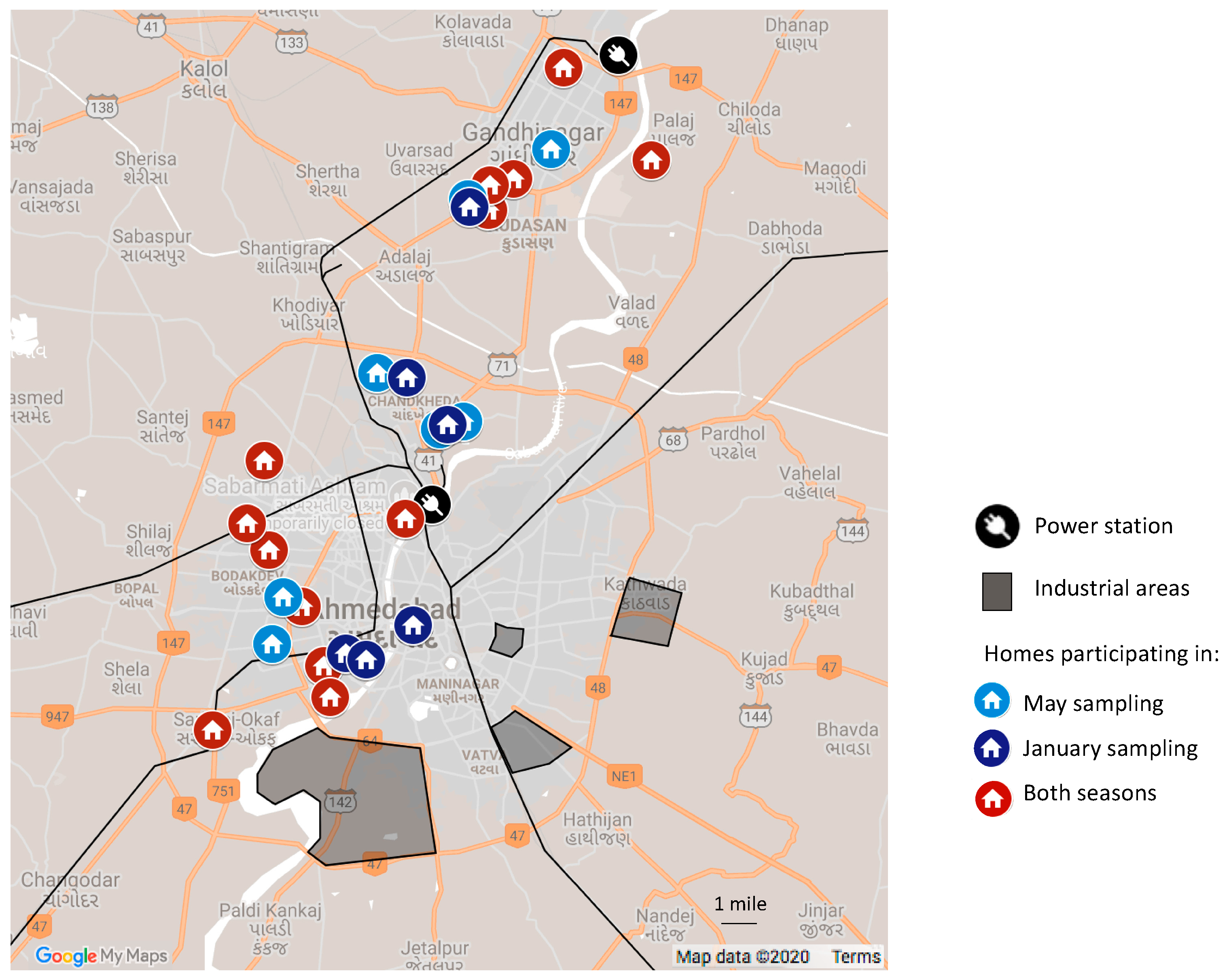
2.1. General Description of the Study Area

Approximately 31% of the population of India resides in an urban area, with a projected increase to 40% by 2030 [40]. Ahmedabad is the 7th largest city in India (population: ~7.8 million in the metropolitan area) and Gandhinagar (population: 292,797 in 2011), situated approximately 30 km north of Ahmedabad, is the capital of Gujarat state [40]. While the Sabarmati River divides Ahmedabad into older (east) and newer (west) districts, Gandhinagar lies solely on its western shores. The Indian Institute of Technology Gandhinagar, a number of small settlements, and the Gujarat International Finance Tec City (GIFT City) are located on the eastern side of the river, across from Gandhinagar proper. Approximately 60% of electricity in India is derived from the combustion of coal and lignite [41], and there are two coal-fired power plants in the area—one on the northern edge of Gandhinagar and the other on the western side of the Sabarmati River in Ahmedabad (Figure 1). In addition, the southeastern part of Ahmedabad contains expanding chemical and petrochemical industries and a large municipal dumpsite (Pirana) [42]. As in other Indian cities, trash and refuse burning are common here [43]. The local vehicle fleet consists of a mix of cars and jeeps, two- and three-wheelers, buses, trucks, and mid-sized vehicles for personal and public transport, and is upwards of 1.4 million [42]. This area is hot and dry during the summer (March-June), with temperatures often in the 40s Celsius, and cooler during the winter (November-February), with temperatures dropping to ~10 °C at night and rising to the mid-20s °C during the day. There is little to no rainfall during these periods.

2.2. Recruitment and Description of Homes

This study involved sample and data collection at 26 homes in Ahmedabad and Gandhinagar, Gujarat, India. We recruited participating households through the networks of our collaborators and local students working on the project and approached individuals from both cities in order to capture the diverse range of sources in this area. Homes with known smokers were excluded. Twenty homes were initially recruited for the study and sampled in May, and although we aimed to re-sample at these homes in January this was not feasible for all homes; 13 homes were re-sampled and six new homes were recruited for sampling in January. The study was approved by the Duke University Institutional Review Board (Protocol number: 2019-0466).
We sampled in apartments (n = 13; on floors ranging from the first to 10th), and row homes/stand-alone homes (n = 13). With two exceptions (a home on the eastern side of the Sabarmati on the campus of the Indian Institute of Technology Gandhinagar and one in the old city in Ahmedabad), all homes were on the west side of the Sabarmati River. Eight homes were in the Gandhinagar area, and 18 were in Ahmedabad (Figure 1). At the furthest, homes were approximately 30 km from each other. With one exception, homes were built between 1995 and 2019 with two homes newly constructed in the last year. Some homes were in predominantly residential areas somewhat removed from shops and the industrial region while others were located on busier roads and in closer proximity to restaurants, stores, and other commercial buildings. Homes were constructed almost exclusively of burnt brick and concrete with mosaic or tile flooring. The kitchens in the homes were either directly connected to the main living area and had no walls to separate them from the rest of the home or were in a separate room with a doorway to the adjacent room. Cooking in all homes was done with liquefied petroleum gas (LPG) or piped natural gas (PNG), with electricity used in a few homes as a secondary means of cooking. All homes used electricity for lighting, and no homes used any sort of air cleaner, be it a stand-alone device or a filter in an air conditioning unit. In one home, there was a smoker who smoked infrequently (i.e., on a monthly basis) but in all other homes there were no smokers and smokers did not visit the houses frequently (i.e., more than once per week).
Two homes had no air conditioning at all, although the majority had either central heating and air conditioning or a secondary type such as a wall-mounted unit. Sampling, which will be described in greater detail in the next section, occurred in the summer (May) and the winter (January). Of the homes with air conditioning, it was used for between 3 and 20 h/day during monitoring in May (mean: ~9 h/day). All homes had windows and/or exterior doors open for some amount of time during monitoring in May (range: 2–24 h, mean: 11 h). In January, windows and doors were always closed in seven homes and were always open in three; overall, doors and windows were closed more often in winter than in summer (mean: 7 h). Participants reported spending some time (range, May: 10–60 min; January: 0–60 min) sweeping/dusting and/or vacuuming during monitoring. In the majority of homes, no renovations had occurred within the year preceding monitoring although at least one room had been re-painted 12+ months prior in many of the homes. In addition to the two homes that had been built in the year preceding monitoring, rooms in one other home had been painted six months prior to monitoring and had been painted three months prior to winter monitoring in another home. One home was being painted on the days that we sampled in January. Participants in these homes are part of a growing middle class in India.

2.3. Overview of Volatile Organic Compound Sample Collection and Analysis

We conducted sampling at homes between 9 May and 23 May 2019 (temperature: 28–45 °C), and between January 10th and 23rd, 2020 (temperature: ~7–30 °C). There was no rain during either period. We collected 90-min integrated air samples on 2,4-dinitrophenylhydrazine (DNPH) (Sigma-Aldrich, Sternheim, Germany; flow rate 0.3 liters per min [LPM]) and Tenax cartridges (Tenax TA, SKC, Eighty Four, PA, USA; flow rate 0.2 LPM) at all homes using SKC AirChek XR5000 pumps and low-flow constant pressure controllers (SKC Inc., Eighty Four, PA, USA). Samples were collected simultaneously indoors in the main room of the home or in a secondary room and outdoors on a balcony or on the front step of the home with the cartridges situated at approximately breathing height using tripods. Once sampling equipment was set up, we used the time-delay function on the pumps to delay the start of the sample collection until the desired start time (i.e., afternoon/evening or early morning). We collected morning samples in all homes during both seasons and afternoon samples in all homes in January. In May, we collected afternoon samples in a subset of 12 homes selected based on project logistics and equipment and participant availability. Morning sampling began between 5:30 and 7:00 am (one exception: start time of 8:00 am at one home). Afternoon/evening sampling events began between 12:45 and 8:00 pm. We calibrated the flow rates in the homes prior to sampling using a MesaLabs Defender 510. Sample collection volumes were calculated using these flow rates and the duration of sampling, and under the assumption that the flow rate remained stable (or increased/decreased linearly) between the initial and final flow calibrations. Shortly after the samples ran to completion, we returned to the homes to check the final flow rates and to seal the sample cartridges prior to transport back to the laboratory; we kept samples on ice during the return journey. We subsequently kept Tenax cartridges in the freezer and DNPH cartridges in the fridge until completion of the field campaign, at which point we transported all samples to the US for analysis by Underwriters Laboratories Inc. Of 140 pairs (i.e., a Tenax/DNPH pair) of samples attempted, all but two ran for the full 90 min. Seventy-eight pairs of samples (for each indoor and outdoor: 20 in May, 19 in January) were collected in the morning and 60 (indoor: 12 in May, 19 in January; outdoor: 12 in May, 17 in January) were collected in the afternoon/evening. We followed the analytical procedures described in previous publications [44,45]. In summary, Tenax TA tubes were thermally desorbed and analyzed by gas chromatography—mass spectrometry. DNPH cartridges were eluted with acetonitrile and analyzed by reverse-phase high performance liquid chromatography with ultraviolet detection. Many of the targeted compounds have an individual LOQ below 1 µgm−3 for an 18 L sample collection volume, however a handful of chemicals (like 1,4-Dioxane and caprolactam) have LOQs slightly higher than 1 µgm−3. To cover all LOQs, the overall LOQ for the VOC analysis was therefore set to be 2 µgm−3. Quality assurance and quality control measures used, and the laboratory analysis of samples are described in the Supplementary text [46].

2.4. Home Survey

We developed a survey to complement the in-home sampling (the complete survey can be found in the Supplementary text). This was used to elucidate factors and sources that may contribute to the compounds measured and their concentrations in and near these homes. Survey questions were based on those used previously in India, or in studies of volatile organic compounds in homes elsewhere [47,48].

2.5. Statistical Analysis

2.5.1. Overview of Concentrations, Detection Rates, and Differences by Location and Sample Collection Time

We examined concentrations of all compounds to identify those prevalent in this area regardless of sampling location, and to determine which compounds were detected only indoors or only outdoors. In addition, we assessed whether concentrations of compounds differed based on the general time of sampling (e.g., morning vs. afternoon/evening). We assessed seasonal differences in the compounds detected and the concentrations at which they were measured. We calculated total VOCs (TVOC) and conducted the analyses discussed above for TVOC as well to investigate temporal and spatial differences.

2.5.2. Non-Negative Matrix Factorization and Investigation of Pollutant Sources

We used non-negative matrix factorization (NMF), a variable reduction technique, to investigate potential sources of the compounds measured. This method has been described previously [49], as has its application to similar data, for the purpose of source identification [45]. In brief, a matrix of samples by concentrations of compounds measured in each sample is decomposed into two matrices that, when multiplied, roughly approximate the input data. The first matrix contains underlying features (e.g., sources or underlying factors that influence concentrations) and an indication of which compounds define or load most highly onto these features, while the second matrix comprises these same features and the level of expression of each of these features in the individual samples. Feature identification was undertaken by selecting the compounds that loaded most highly onto each of the features and by examining, in the literature from both India and elsewhere, typical sources of these compounds and especially sources that emit these compounds in concert. The temporal and spatial patterns of expression were also used to identify factors (e.g., a factor that is expressed most strongly indoors is unlikely to represent vehicle exhaust but may rather point to indoor sources such as consumer or cleaning products). Source analyses were restricted to compounds detected five times or more above the limit of quantitation (LOQ; 2 µgm−3).

3. Results

3.1. Overview of Compounds Measured

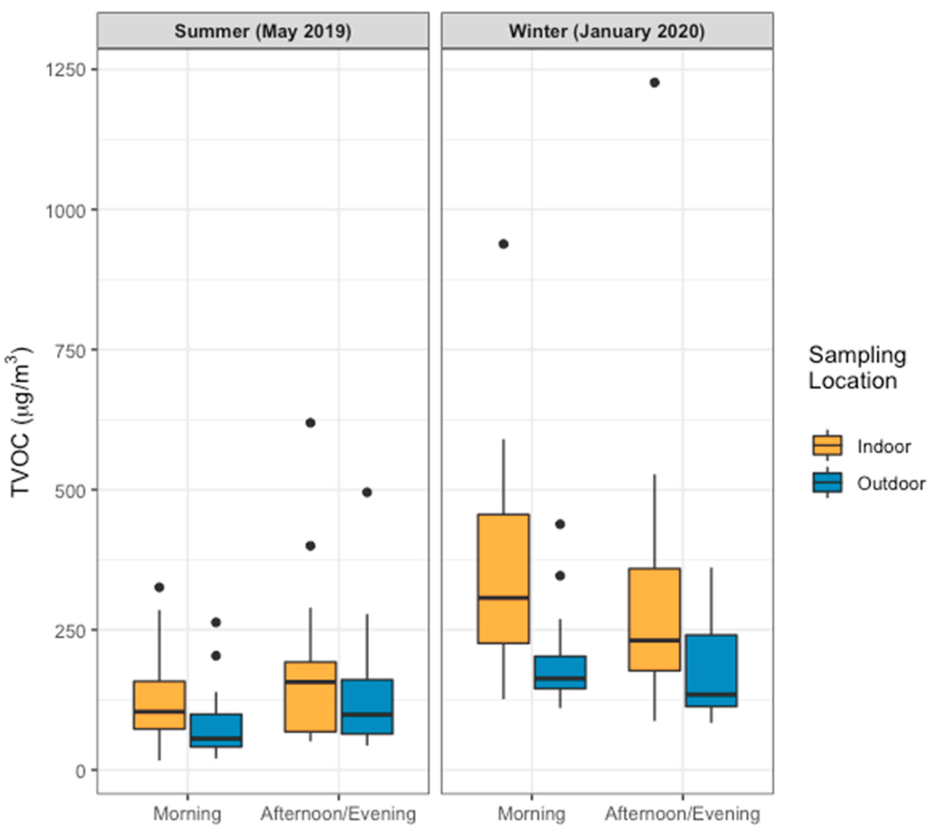
3.1.1. Total Volatile Organic Compounds

TVOCs were higher indoors than outdoors in the morning (paired Wilcoxon signed rank test, p < 0.05) during both seasons (Figure 2). This may be due to a reduction in emissions from some sources overnight (e.g., traffic, industry). In addition, compounds emitted indoors during this time may persist indoors if the home is closed or partially closed overnight. For samples collected in the afternoon/evening, differences between indoor concentrations and outdoor concentrations were not significant at the α = 0.05 level in May (n = 12), although they were significant in January (n = 19). These seasonal differences may result from behavioural differences; in May, temperatures were frequently in the low 40s °C. In most homes the doors and windows were open during the day to encourage airflow and many people were using ceiling fans. These practices likely facilitated the circulation of ambient air indoors, and of indoor air outside leading to more complete mixing of the indoor and outdoor pollutants over the course of the day. This in turn resulted in less distinct indoor-outdoor patterns in these environments than were seen in January, and in our previous work in China [45]. In contrast, during the winter families may have encouraged differences in pollutant concentrations in these two environments to persist over a longer period of time by keeping some or all doors and windows closed.
For both indoor and outdoor sampling, concentrations were lower in the morning than in the afternoon/evening in May, although the opposite was observed in January. In previous work in Ahmedabad, researchers found that biogenic emissions of certain compounds (e.g., isoprene) follow temperature trends [50]. As such, some of the morning/late-day differences observed for May might relate to the increase in temperature that occurred over the course of the day, with temperatures usually dipping to 28 or 29 °C around 6 am and then increasing to 40–43 °C by mid-afternoon. In addition, in the previous work in Ahmedabad there were peaks in VOCs during the morning and evening, with some of these likely relating to traffic [50]. For some VOCs, especially those with outdoor sources, higher concentrations in the morning may relate to changes in boundary layer height and the stagnation of air flow overnight [50]. Similarly, some of the seasonal differences observed (e.g., with higher concentrations observed outdoors during winter sampling than during summer sampling) may relate to seasonal differences in the height of the boundary layer [51].
Lastly, concentrations of TVOCs were generally higher in January than in May. A lower mixing height in the winter may have led to higher concentrations of pollutants during this time. This seasonal difference is also consistent with previous work in India in which pre-monsoon concentrations of TVOC were lower than post-monsoon concentrations due to the high solar radiation in the pre-monsoon period which, indirectly, leads to the degradation of VOCs [52].

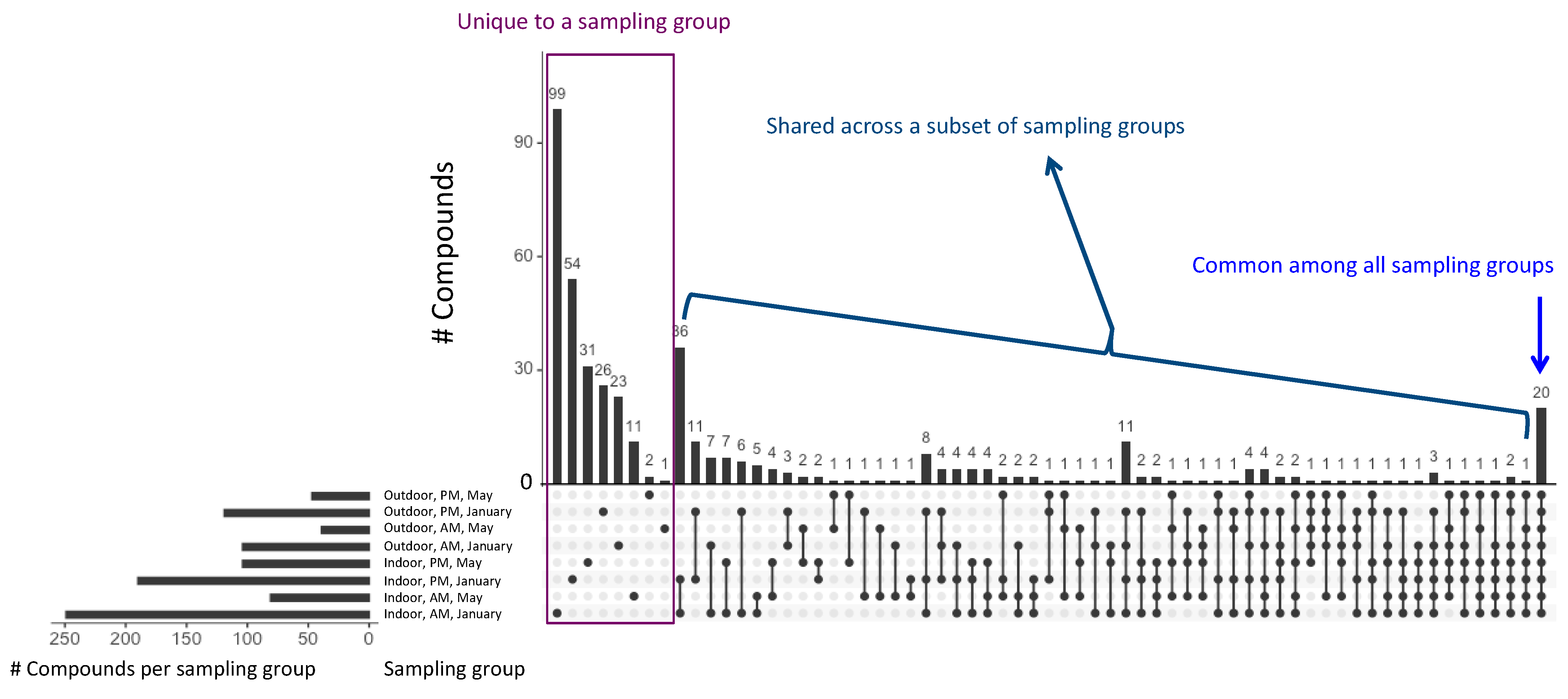
3.1.2. Individual Compounds: Prevalence and Temporal and Spatial Patterns

Although nearly 700 compounds were identified in May and nearly 950 were identified in January, only 149 and 380 compounds were measured above the LOQ in May and January, respectively. These compounds will be the focus of our analyses, with particular emphasis on compounds measured five times or more (n = 69, Table S1). Indoors, 381 compounds were detected at least once and outdoors, 181 compounds were detected at least once. Similar to what we observed in China during a study employing the same methods, some compounds were nearly ubiquitous across homes [45]; acetaldehyde was measured in all samples and formaldehyde was measured in all but one sample. In addition, 2,2,4,6,6-pentamethylheptane was measured in all samples in January, and in 72% and 84% of indoor and outdoor samples, respectively, in May.
As expected, there were also differences in the compounds that were measured by location, pointing to unique sources in these environments; 258 compounds were measured indoors but never outdoors and 58 were measured outdoors but never indoors. In Figure 3, we highlight the overlap between compounds detected at different times of day, in the two seasons, and indoors versus outdoors. While 20 compounds were measured in all sampling groups (with a sampling group defined by season, location, and time of day, e.g., all samples measured indoors, in the morning, in May; n = 8 total sampling groups), there were many compounds that were unique to each group. As a group, samples collected indoors in the morning in January had the highest number of compounds detected (n = 249) with 99 compounds measured exclusively in this sampling group. This may result from many families keeping their doors and windows closed overnight in the winter leading to a buildup of compounds during this time.
The diversity of compounds measured and the differential overlap between sampling groups (Figure 3) illustrate the complexity of air quality in these environments; a wealth of sources exists indoors, and the range of compounds measured indoors far outstrips those measured outdoors. Lastly, this highlights the importance of considering seasonal and diurnal effects when assessing air quality. To further investigate these differences by season, sampling time, and sampling location, we used paired Wilcox exact tests to determine whether, for compounds that were measured in two sampling groups, the differences in the concentrations were significant. For each comparison, a subset of compounds had statistically significant differences at the α = 0.05 level; the results of these tests are provided in Table 1. These comparisons were done for all compounds but only the compounds with statistically significant differences are listed in Table 1. For indoor samples, differences by time of day in May could be attributed to greater cooking activity prior to or during the afternoon/evening session than during the morning sampling session as aldehydes including decanal and nonanal have been previously identified as compounds emitted during rice cooking [53]. Temporal differences in ambient compounds may relate, in part, to diurnal patterns of vehicle traffic. In additional Ahmedabad-based work, researchers have shown that there is large diurnal and day-to-day variation in the concentrations of individual VOCs. In the aforementioned work the concentrations observed were bi-modal, with morning (8–10 h) and evening (18–21 h) peaks for compounds with anthropogenic sources and with slightly delayed peaks (from 10–12 h) for acetone and acetaldehyde, pointing to their photochemical generation from primary emissions [54]. In our work, seasonal differences likely relate to changes in the sources themselves (i.e., there is likely to be more heating occurring during the winter, and the products used in these two seasons might differ) and to the behaviours of families (i.e., window/door opening; fan use). Some differences might also be attributable to seasonal environmental factors (e.g., strength and direction of prevailing winds). Patterns of the compounds measured and identification of possible sources of these compounds are discussed in greater detail in Section 3.2.

3.1.3. Hazardous Compounds

Of the compounds measured above the LOQ, 46 present a potential inhalation health risk as outlined by the California Office of Environmental Health Hazard Assessment (OEHHA) [55], the International Agency for Research on Cancer (IARC) [56], and/or the US EPA’s Integrated Risk Information System (IRIS) [57] (Table S1). All but one of these compounds were measured indoors. Two of these compounds—benzene and formaldehyde—are known human carcinogens (i.e., IARC Group 1 compounds). Two others—N,N-dimethylformamide and styrene—are probable human carcinogens (Group 2A compounds under IARC) and nine compounds (acetaldehyde; naphthalene; 1,4-dichlorobenzene; 1,4-dioxane; methyl isobutyl ketone; cumene; benzofuran; ethylbenzene; benzophenone) are possible human carcinogens (i.e., IARC Group 2B compounds). The health effects of exposure to compounds listed in the OEHHA database range from acute effects such as nausea, dizziness, headache, and respiratory and eye irritation to longer-term reproductive and developmental effects [55]. It is of particular concern that for a number of these compounds (e.g., formaldehyde, toluene) the concentrations measured inside exceed those measured in ambient air.
Acetaldehyde and formaldehyde were two of the most prevalent hazardous compounds measured indoors in our study and in previous work. The median and maximum concentrations of acetaldehyde measured in our study were comparable to those measured in Los Angeles in the fall (our study—median [max.], winter: 10.57 [23.88] µgm−3; summer: 9.02 [28.15] µgm−3; Los Angeles—median [max.]: 8.6 [23] µgm−3), although the concentrations measured in Los Angeles in the winter were slightly higher than ours (median [max.]: 15 [36] µgm−3) [58]. From this same study, the maximum concentrations measured in New York in both the summer and winter exceeded those measured in either season in our study, although the median values were only slightly higher than ours (median [max.], winter: 14 [54] µgm−3; summer: 11 [92] µgm−3). Our concentrations were lower during both seasons than the concentrations we measured indoors using the same methods in Shanghai, China (13.9 [207.9] µgm−3) [45]. In general, our concentrations overlap with those measured by others sampling at homes in Europe and the United States, although the maximum concentrations in other studies were higher than those measured in the current work [59].
In 2010, based on studies of exposure to formaldehyde and the associated health effects, the World Health Organization established an indoor air quality guideline for short- and long-term exposures to formaldehyde; the guideline was set at 0.1 mgm−3 for all 30-min periods at lifelong exposure. Median concentrations in our study fall well below this guideline value, although concentrations at some individual homes (n = 3 instances; 2 homes) were higher. Further, a 2010 review of formaldehyde in the indoor environment highlighted how variable the concentrations of this compound can be even in indoor environments—in a number of studies, concentrations were in the single digits but in kitchens in Turkey they were as high as 2086 µgm−3 [60]. Concentrations indoors in our study in May (median [max.]: 22.73 [211.82] µgm−3) exceeded those measured in a study in New York (winter: 12 [22] µgm−3; summer: 19 [51] µgm−3) and Los Angeles (winter: 18 [59] µgm−3; summer: 15 [32] µgm−3) [58]. Although they were much higher than concentrations measured in classrooms in Sweden (<5–10 µgm−3) [61], our maximum concentrations were comparable to those measured in homes in Australia (mean [max.] in child’s bedroom: 30.2 [224] µgm−3; mean in living room: 27.5 [189.7] µgm−3) [62]. In the current work, concentrations in India in May and the median concentration in January (25.85 µgm−3) were slightly higher than what we measured indoors in the spring in China (17.9 [137.5] µgm−3). Overall, our concentrations are not drastically different than those measured previously indoors, and instead further reflect variability between concentrations in indoor spaces already recorded in the literature. Understanding and quantifying this variation—with some homes exceeding guideline values for harmful pollutants although, on average, homes did not—is critical when thinking about how to limit exposure to these harmful pollutants.
Naphthalene was measured indoors in 47% of samples in May and in 84% of samples in January. In addition, the maximum values measured were quite high (109.21 µgm−3 in May and 140.89 µgm−3 in January). These values far exceed the WHO guideline value of 10 µgm−3 for annual average concentrations [63]. The use of mothballs in the home might explain the naphthalene measured in some homes—the home with the highest concentration in January reported always using mothballs—but it does not explain all the variations observed as, for example, the home with the highest concentrations in May reported never using mothballs. Naphthalene is also used in some paints and in some other pesticides [63].
Lastly, benzene—detected in 65% of indoor samples in our previous work employing the same sampling strategy in China—was detected in 6% and 87% of indoor samples in May and January, respectively, in the current study. This further illustrates the importance of understanding geographic and temporal variation in the prevalence and concentrations of these health-relevant compounds.

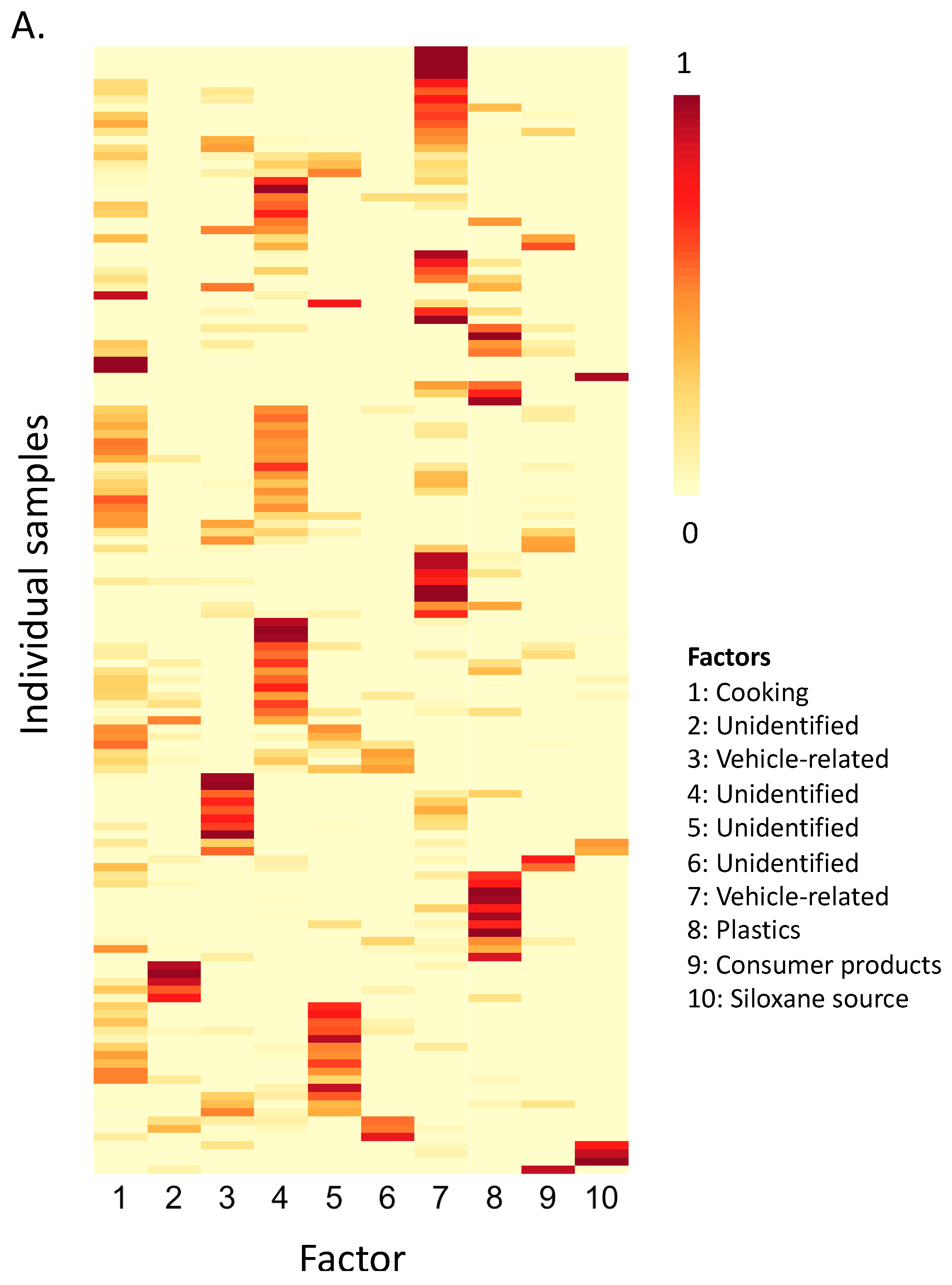
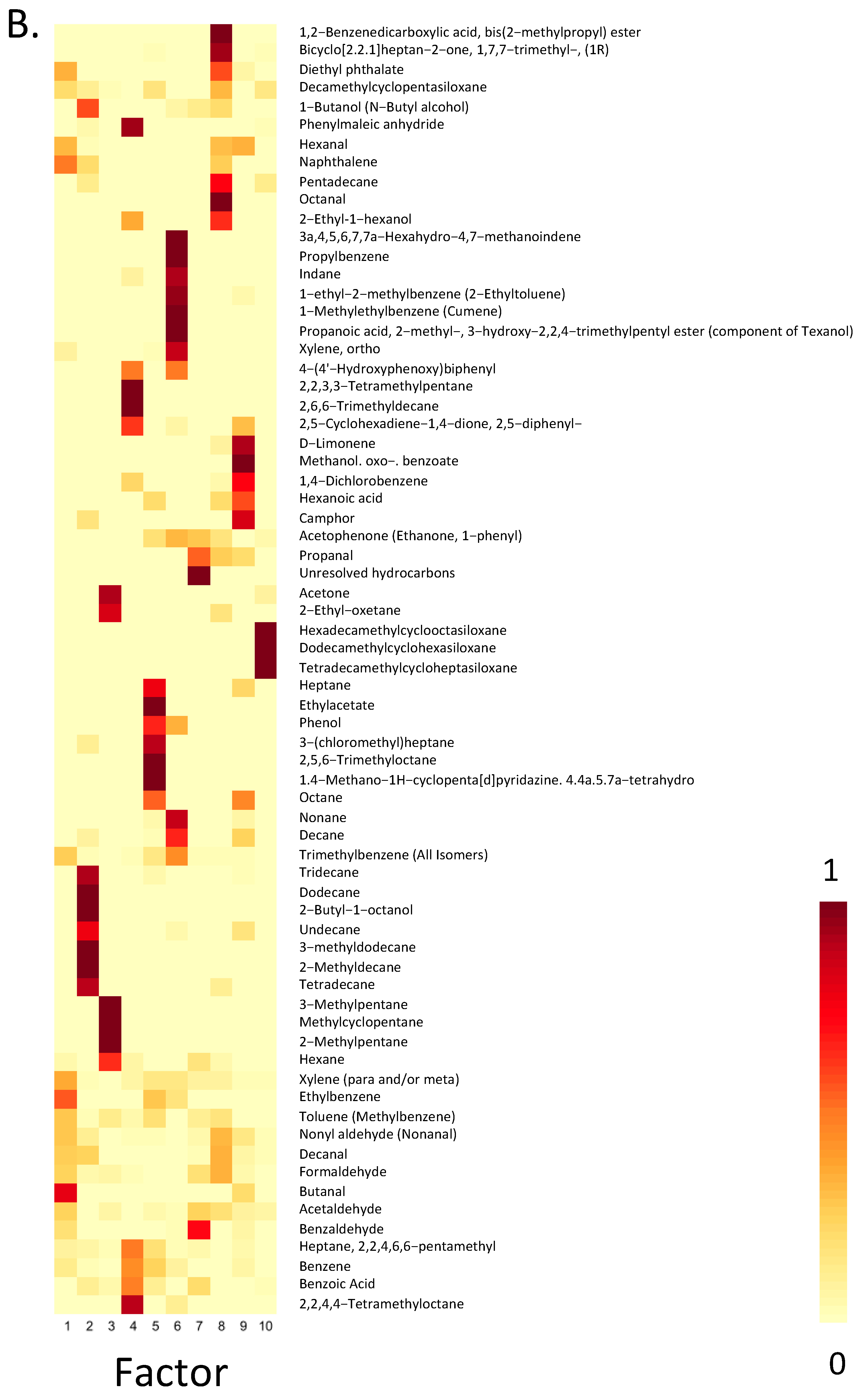
3.2. Source Identification Using Non-Negative Matrix Factorization

Given the complexity of the data, we used non-negative matrix factorization—a variable reduction tool—to identify compound groupings that may represent sources or point to factors (e.g., environmental conditions) that affect compound emissions. With data from both seasons combined (n = 138 samples), restricting to compounds measured above the LOQ five times or more (n = 69), and based on adjusted Eigenvalues >1, we extracted ten underlying features from the data set which explained approximately 64% of the variance in the data. As has been pointed out previously, while these clusters or factors represent one solution to the matrix decomposition, this is not the only solution [64]. Our identification of the factors followed from an examination of the sampling locations (e.g., indoor or outdoor), times (e.g., morning or afternoon/evening) and seasons during which these factors were expressed most strongly (Figure S1, Figure 4 and Figure 5), combined with the compounds that loaded most highly onto each of the factors. Factor interpretations are outlined in the following sections.

3.2.1. Factor 1: Cooking

This factor was represented more in indoor than outdoor samples, although it was present in both. It had higher loadings in January than in May, and was defined by high loadings of butanal, ethylbenzene, naphthalene, diethyl phthalate and hexanal. All of these compounds have been associated with rice [65], and a few are associated with cooking with oils at high temperatures [15]. Seasonal differences in this factor may relate to differences in how open the homes were during these periods, allowing for more (May) or less (January) dispersion of the compounds emitted during cooking activities indoors. Outdoor samples with high expression of this factor may indicate contributions from street vendors or individuals cooking outdoors, as both were commonly observed. It is also possible that some of the compounds emitted indoors migrated outdoors during the cooking process if the windows or doors were open.

3.2.2. Factor 3: Vehicle-Related

This factor was represented more outdoors than indoors, and in the afternoon/evening than in the morning. It was stronger in May than in January. Compounds defining this factor include 2-methylpentane, 3-methylpentane, methylcyclopentane, hexane, acetone and 2-ethyloxetane. Some of these compounds have been measured in the exhaust of 2-wheelers [66], which were commonplace in the streets near these homes, while others have been measured in vehicle exhaust in general [67]. These profiles—with some representation indoors—point to the ability of ambient pollutants to infiltrate homes, especially when doors and windows remain open for extended periods of time (e.g., in May). Although benzene is often associated with gasoline and vehicles, there has been a push to remove benzene from gasoline in India; it is thus not surprising that benzene does not load as highly onto these vehicle-related factors as might be expected in other locations or as would have been expected in the past [68].

3.2.3. Factor 7: Vehicle-Related

Similar to factor 3, this factor was strongest outdoors, although it was also measured indoors in May. It had little representation indoors in January, when we expect homes to be better sealed than in the summer. It was associated most strongly with unresolved hydrocarbons, propanal, and benzaldehyde, which have been measured at petrol pumps in Kolkata, India [69]. Although this factor and factor 3 both appear to be related to the emissions of vehicles, it is possible that the differences highlight a shift in the vehicle fleet over the course of the day, or that this factor relates partly to activities taking place at/emissions from vehicle refueling stations.

3.2.4. Factor 8: Plastics

This factor was identified predominantly indoors in May, although it was still detected indoors a number of times in January. It was seldom detected outdoors in either season. Compounds common to this factor include di-isobutyl phthalate and diethyl phthalate—plasticizers which have been measured in dust in homes, child-care facilities and salons in the United States [70]—and 2-ethyl-1-hexanol, which is produced by the microbial degradation of plasticizers [71]. Plasticizers are generally used to make products more flexible and the phthalate class of compounds is widely used to this end [72]. This factor also had high loadings of (1R)-1,7,7-trimethylbicyclo [2.2.1] heptan-2-one (aka D-camphor) and pentadecane; pentadecane and camphor isomers have been associated with plastic products [73]. Octanal also loaded highly onto this factor. This factor may relate to the off-gassing of plastics, which may occur more readily at the high temperatures observed in May than in January.

3.2.5. Factor 9: Consumer Products

This factor had low representation in general, but was highest indoors, in the morning, in January. It had high loadings of octane; camphor; hexanoic acid; 1,4-dichlorobenzene; methanol. oxo-. benzoate; and D-limonene. Camphor and limonene have been associated with fragranced consumer products [13,74]; hexanoic acid has been associated with odors, including from latrines and farms with livestock [75], and measured in trace amounts in seaweed collected in Tamil Nadu, India [76]; and 1,4-dichlorobenzene is sometimes emitted from mothballs, essential oils, and other consumer products [36]. These compounds may point to the use of consumer products during the winter, and the fact that compounds may be more likely to linger indoors during the winter if the home is closed.

3.2.6. Factor 10: Siloxane Source

This factor was expressed almost exclusively outdoors, during the later-day sampling sessions in May. Siloxanes (hexadecamethyl-cyclooctasiloxane [D8], dodecamethyl cyclohexasiloxane [D6], and tetradecamethyl-cycloheptasiloxane [D7]) loaded most highly onto this factor. Siloxanes including D6, D7, D8 and decamethylcyclopentasiloxane (D5) have been measured previously in dust collected indoors in Patna, India, and in other countries [77], and are a common component in household products including electronics, furniture, and cookware [78]. They are also found in health-care products, cosmetics (e.g., deodorants, anti-perspirants, hair care products, foundation), and medical devices, with their ubiquity in a diverse range of products stemming from the low surface tension, high thermal stability, and smooth surface of silicone products [78]. However, their prevalence in these products and thus their manufacture has led to siloxanes being measured in ambient air globally, even in parts of the world with very low populations (e.g., the Arctic) [79]. As such, this factor may indicate emissions from the production of these types of products.

3.2.7. Unidentified Factors

A number of factors were unidentified, although related to some sampling groups but not others (e.g., based on season, time of day). Factor 2 was strongest indoors in January, and compounds that loaded the most highly onto this factor (tridecane, dodecane, undecane and tetradecane) have been measured previously in pesticides [80]. However, these and other compounds on this factor (3-methyldodecane and 2-methyldecane), have also been associated with chickpea seeds and roasted chickpea [81,82]. 1-butanol, which also loaded highly onto this factor, was measured in indoor (workplace, home) environments in Finland, where authors indicated it might relate to paint and the presence of mold or bacteria in these environments [21], but it has also been associated with rice bran and scented rice [65]. 2-butyl-1-octanol also loads onto this factor. Seasonal differences such as those observed here may point to differences in the products that are used indoors in the winter and summer, or to differences in behaviours (e.g., seasonal variation in the foods cooked). Our winter sampling campaign overlapped with the kite festival—a holiday enjoyed broadly in Gujarat. Certain foods are made specifically for this festival.
Factor 4 differed greatly by season, with much stronger representation in January than in May and slightly higher representation outdoors than indoors in May. There is no clear indication of common sources of the compounds defining this factor (see Table 2 for compounds).
Factor 5 was strongest in the morning (indoors and outdoors) and had much stronger representation in January than May. Octane and 3-(chloromethyl)heptane, which loaded strongly onto this factor, have been measured in Nardostachys jatamansi DC, a plant found in India that is used for its medicinal properties, and which is sometimes used in essential oils [83]. Octane has also been measured during ritual burning in India [39], and during stir-frying of vegetables in soybean oil [84]. Given how strong this factor was in the morning, but almost exclusively in January, it is possible that it relates to a seasonal ritual that only takes place in the morning. It is also possible that some of the unidentified factors that are stronger outdoors reflect some of the trash and refuse burning observed in the city—burning may be more common in the winter on cool mornings as a source of heat than at other times of day or in other seasons.
Factor 6 had low representation in general, being most strongly represented in four homes. It was expressed more in January than in May. Texanol, which loaded highly onto this factor (see Table 2 for other prominent compounds) is a component of paints [85], and one of the homes was being painted during the days that sampling occurred. This home had the strongest loading of this factor in all samples in January, although it was not represented in this same home during May sampling—prior to the painting. One of the other four homes had been fumigated prior to sampling, and there were closed paints being stored in the home. At this same home, two rooms had been painted in the past year, but it was unclear exactly when.

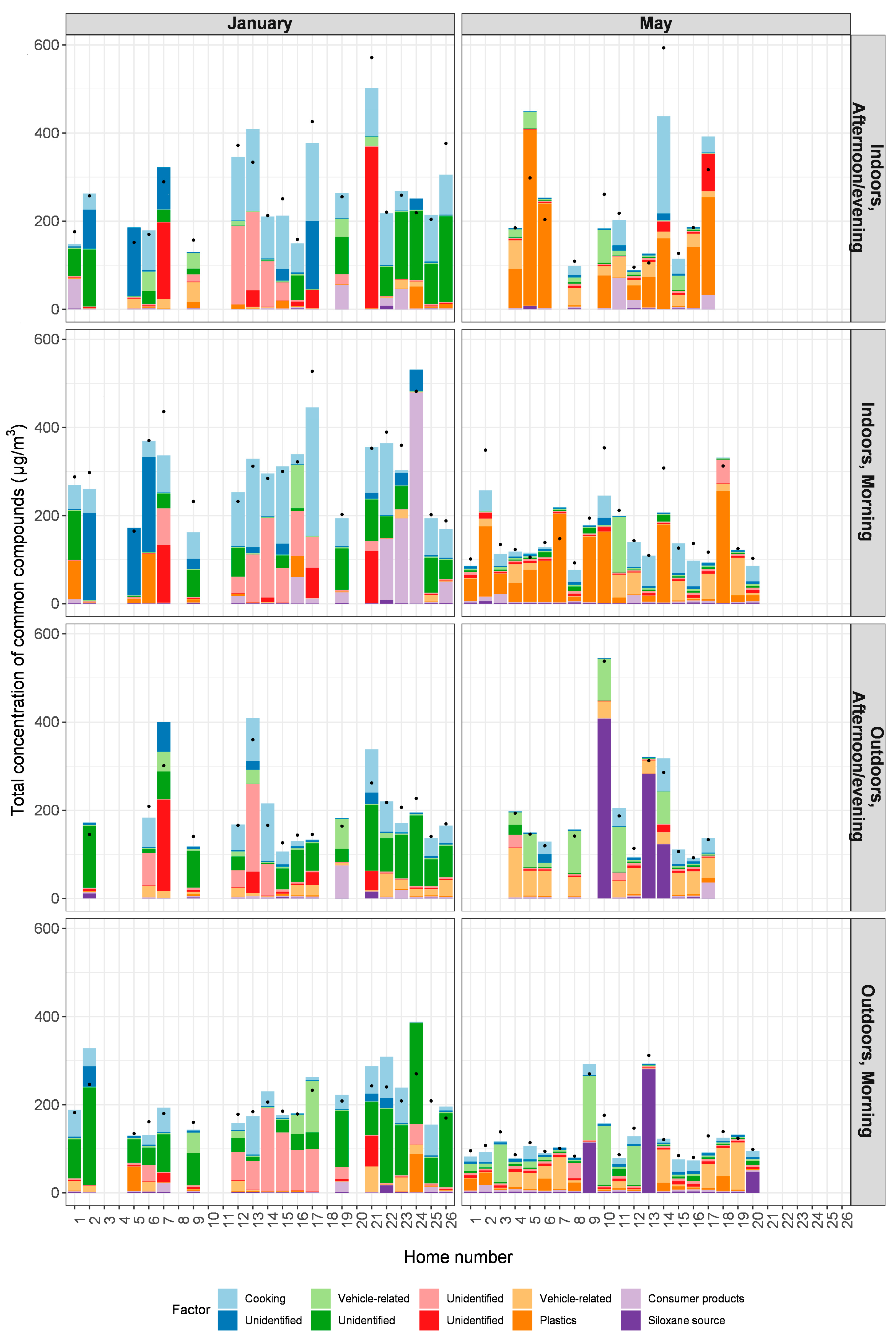
3.3. Factor Contributions

Contributions from each of the 10 factors varied greatly between samples (Figure 5). There were noticeable trends by season and by sampling location; in May, contributions from plastics appeared to be much greater than in January, especially for indoor samples. This was consistent for indoor samples regardless of time of day at which the sampling was done and may relate to greater off-gassing of compounds during the hotter temperatures. Some sources such as the siloxane source and consumer products had very strong representation in a small number of homes, with much smaller contributions in other homes. Contributions from cooking were more noticeable in January than in May and were reflected more in indoor than in outdoor samples. In January, when the temperatures were cooler, homes were more likely to have doors and windows closed. Of note, not all homes had sampling done in each of these locations for all times; this is reflected in gaps in bars missing for some homes in Figure 5.

4. Discussion

Many compounds that we quantified have also been measured in previous work in India. Phthalates including di-isobutyl and diethyl phthalate were previously measured with concentrations higher during summer than winter [86]. Authors speculated that the seasonal differences observed may relate to the higher temperatures during summer; these compounds are often used as plasticizers but are not chemically bonded to the polymer making it possible for them to evaporate. Some of these compounds are also emitted when plastics are burned, as is frequently the case in India; during the sampling campaign, evidence of trash burning or the practice itself was observed throughout the city and over the course of the day. In our work, concentrations of diethyl phthalate differed by sampling location in January and differed between seasons for samples that were collected indoors in the morning. In this same study, the authors observed higher concentrations of benzoic acid during the day than during the night and attributed these temporal differences to a photochemical source [86]. We observed a similar trend in May, with concentrations of benzoic acid typically higher during later day than morning sampling sessions. Our ambient values for benzene contrast with those measured at three different sites in Kolkata, where the mean values ranged from 24.97 to 79.18 μgm−3 [86]; our values were all <10 μgm−3. In previous work in Ahmedabad, researchers observed a shift in the concentrations of compounds measured between February and March, which they indicated was the transition from winter to summer—during the hotter and sunnier months they measured higher concentrations of compounds with photochemical sources such as acetaldehyde and acetone [87]; in the current study, acetaldehyde was measured during all ambient sampling events in both seasons (range of concentrations: 3.63–26.11 μgm−3) but acetone was measured in 34% of ambient samples in May (range of concentrations: <LOQ-21.52 μgm−3), but in only 3% of samples in January and at quite low concentrations (range of concentrations: <LOQ-2.05 μgm−3). Numerous compounds detected in our study (i.e., benzene, toluene, styrene, formaldehyde, acetaldehyde, chlorobenzene, benzaldehyde, propanal, butanal, and hexanal) have been detected at municipal waste sites in India [88]. It is possible that the Pirana landfill in the south of Ahmedabad contributed to some of the concentrations being measured in our work, although there was no clear signal in our analyses. This may, in part, be due to the relatively small sample size and the geographic distribution of the homes, as well as differences in the prevailing winds in these seasons. The winds may push contaminants from the landfill away from homes in one season but towards some homes in the other season.
We compared our findings with previous concentrations measured indoors as well. In previous work in non-residential, indoor, public spaces (i.e., an office, food courts, theaters, a restaurant, a conference room and a bar), concentrations of benzene were as high as 113.89 μgm−3 [37]. In contrast, they were between <LOQ and 9 μgm−3 in our study. Naphthalene—a possible carcinogen—was consistently below 0.1 μgm−3 in public spaces during previous work but was measured in 47% of indoor sampling events in May and 84% in January in our study although there were discrepancies in concentrations between duplicates. In a study of university-provided housing for staff and students in India [36], concentrations of toluene were higher, on average (mean in living room: 32.9 μgm−3), than in the current study (mean in May: 7.90 μgm−3; January: 11.05 μgm−3).
These important discrepancies between our findings and those of others in India may be in part because the materials and products used in public spaces and campus housing do not reflect those used in residential spaces, and the behaviours of individuals may differ between these environments. This highlights the importance of conducting research in these unique spaces. As most time spent indoors is spent at home and the majority of people in India are not living in student dormitories, quantifying pollutants in non-dormitory residential environments is particularly relevant to understanding exposures and their consequences on a broader scale.
To our knowledge, this is the first work done to quantify such a diverse range of VOCs inside and outside homes in urban India that do not rely on biomass fuels for cooking and heating, and to do so in two seasons. As such, although our sample size was somewhat small (n = 26 homes) this work provides much needed insight about indoor air quality in these spaces and how this relates to ambient air quality; given the time spent indoors at home, pollutants in these environments can have a disproportionately large effect on health. While our work begins to fill this void, it has a number of limitations. Our 90-min samples only provide a snapshot of the pollutants in the homes at a particular time of day. In addition, although it would have been beneficial to standardize the sampling start times, this was not feasible in the current study given logistical constraints related to equipment and personnel, time commuting to and between sites, and the schedules of study participants. Having sampled only for one morning and one afternoon at each home (in each season), we are unable to account for day-to-day differences in the concentrations of VOCs at these homes. To address this, future work should include repeat sampling in homes at the same time of day but on different days. A strength of our work is that by doing both morning and evening sampling on the same day at a subset of homes in May and for all homes in January we were able to capture some of the differences we might expect to see over the course of a day. For example, pollutant composition and concentrations may change throughout the day due to the photochemical generation of VOCs, changes in temperature and humidity that lead to increased off-gassing of VOCs, and because many VOCs are emitted by products used by humans on short time scales (e.g., personal care products) or are associated with human behaviours such as opening windows and activities such as cooking. We anticipated seasonal differences in pollutant concentrations due to changes in meteorological factors (e.g., wind direction), shifts in pollutant sources (e.g., perhaps there is more combustion for heating in the winter) and human behaviours over the course of the year. By sampling in two seasons, we were able to capture some of these differences and their effect on both indoor and outdoor air quality. Of note, our approximately two weeks of sampling in each season may not represent the full seasonal profile—extended sampling in each season is warranted. Quantifying these temporal, indoor/outdoor, and geographic patterns of pollutants is crucial in the context of health and thinking about interventions that could be used to improve air quality in these environments. Lastly, additional sampling at ambient sites could facilitate the interpretation of pollutant sources by allowing for better identification of source fingerprints in this region.

5. Conclusions

In summary, we measured VOCs indoors and outdoors at 20 homes in May and 19 homes in January in Gandhinagar and Ahmedabad, India, during early morning sampling sessions in all homes and during afternoon/evening sampling sessions in a subset of 12 homes in May and at all homes in January. There was large variability in the concentrations of VOCs measured across homes, although in general concentrations were higher in the later-day sampling sessions compared to the morning sessions in May, and higher indoors than outdoors in both seasons. Ten potential source groupings were identified for compounds detected at least five times, although for some of these groupings there was not a single clear underlying source or factor. Factors identified related to cooking, plastics, consumer products, siloxanes, and vehicles. It is worthwhile to note that plastic sources contributed substantially to poor indoor air quality in May but not January, pointing to potential impacts of off-gassing at higher temperatures. The large number of compounds quantified above the LOQ that have previously documented adverse associations with health highlights the importance of understanding where these compounds are coming from and how prevalent they are in the indoor environments where people spend the majority of their time. This work represents a first step towards quantifying indoor VOCs in Indian cities and their contribution to poor air quality and associated health impacts.

Supplementary Materials

The following supporting information can be downloaded at: https://www.mdpi.com/article/10.3390/environments9070075/s1. Figure S1. Concentrations of compounds detected five times or more (n = 69) across all samples (n = 138), with concentrations scaled by centering and standardizing each column separately to column Z-scores. Samples have been grouped by season (May, January) and sampling location (indoor, outdoor) to best illustrate trends. Table S1. Summary of all compounds detected 5 times or more above the LOQ of 2 µgm−3 in May or in January; ordered by frequency of detection indoors in January. Where a minimum or median value of 1 is presented, this is because the minimum or median value was below the LOQ.

Author Contributions

Conceptualization, M.H.B., J.J.S., R.E., C.G. and C.L.N.; methodology, M.H.B., J.J.S., R.E., C.G., C.L.N. and M.B.; formal analysis, C.L.N.; investigation, C.L.N. and R.E.; resources, M.H.B., J.J.S., C.G. and M.B.; data curation, C.L.N.; writing—original draft preparation, C.L.N.; writing—review and editing, M.H.B., J.J.S., R.E., C.G., C.L.N. and M.B.; visualization, C.L.N. and M.H.B.; supervision, M.H.B. and J.J.S.; validation, M.H.B., J.J.S., C.L.N., R.E., M.B.; project administration, M.H.B., J.J.S., R.E., C.G. and C.L.N.; software, C.L.N., funding acquisition, M.H.B. and J.J.S. All authors have read and agreed to the published version of the manuscript.

Funding

This research was funded by Underwriters Laboratories Inc. (UL).

Institutional Review Board Statement

The study was conducted in accordance with the Declaration of Helsinki, and approved by the Institutional Review Board of Duke University (protocol number: 2019-0466, March 2019).

Informed Consent Statement

Informed consent was obtained from all subjects involved in the study.

Data Availability Statement

The data presented in this study are available on request from the corresponding author.

Acknowledgments

We gratefully acknowledge the families who welcomed us into their homes for sampling and who worked with us to complete the household surveys. Sampling would not have been possible without our students (Aniket Ratnaparkhi, Haimi Jagirdar, Priyansh Singh, Sanjeet Yadav, and Darpan Lakhmani, Drashti Dave, and Dharmil Shah) who sorted out logistics, ensured we made it to the homes, and assisted with monitoring.

Conflicts of Interest

The authors declare no conflict of interest. The funders had no role in the design of the study; in the collection, analyses, or interpretation of data; or in the decision to publish the results.

References

  1. Mukhopadhyay, K.; Forssell, O. An empirical investigation of air pollution from fossil fuel combustion and its impact on health in India during 1973–1974 to 1996–1997. Ecol. Econ. 2005, 55, 235–250. [Google Scholar] [CrossRef]
  2. Pandey, J.; Agrawal, M. Evaluation of air pollution phytotoxicity in a seasonally dry tropical urban environment using three woody perennials. New Phytol. 1994, 126, 53–61. [Google Scholar] [CrossRef]
  3. Beig, G.; Chate, D.M.; Ghude, S.D.; Mahajan, A.S.; Srinivas, R.; Ali, K.; Sahu, S.K.; Parkhi, N.; Surendran, D.; Trimbake, H.R. Quantifying the effect of air quality control measures during the 2010 Commonwealth Games at Delhi, India. Atmos. Environ. 2013, 80, 455–463. [Google Scholar] [CrossRef]
  4. Greenstone, M.; Harish, S.; Pande, R.; Sudarshan, A. The Solvable Challenge of Air Pollution in India. In Proceedings of the India Policy Forum, New Delhi, India, 11–12 July 2017. [Google Scholar]
  5. Balakrishnan, K.; Dey, S.; Gupta, T.; Dhaliwal, R.S.; Brauer, M.; Cohen, A.J.; Stanaway, J.D.; Beig, G.; Joshi, T.K.; Aggarwal, A.N.; et al. The impact of air pollution on deaths, disease burden, and life expectancy across the states of India: The Global Burden of Disease Study 2017. Lancet Planet. Health 2019, 3, e26–e39. [Google Scholar] [CrossRef] [Green Version]
  6. Sarkar, S. India Launches a National Clean Air Program. Available online: https://www.nrdc.org/experts/anjali-jaiswal/india-launches-national-clean-air-program (accessed on 7 September 2019).
  7. Gaur, M.; Singh, R.; Shukla, A. Volatile Organic Compounds in India: Concentration and Sources. J. Civ. Environ. Eng. 2016, 6, 23–27. [Google Scholar] [CrossRef] [Green Version]
  8. Kjærgaard, S.K.; Mølhave, L.; Pedersen, O.F. Human reactions to a mixture of indoor air volatile organic compounds. Atmos. Environ. Part A Gen. Top. 1991, 25, 1417–1426. [Google Scholar] [CrossRef]
  9. Ware, J.H.; Spengler, J.D.; Neas, L.M.; Samet, J.M.; Wagner, G.R.; Coultas, D.; Ozkaynak, H.; Schwab, M. Respiratory and irritant health effects of ambient volatile organic compounds. The Kanawha County Health Study. Am. J. Epidemiol. 1993, 137, 1287–1301. [Google Scholar] [CrossRef]
  10. LBNL. VOCs and Cancer. Available online: https://iaqscience.lbl.gov/voc-cancer (accessed on 10 April 2018).
  11. Huangfu, Y.; Lima, N.M.; O’Keeffe, P.T.; Kirk, W.M.; Lamb, B.K.; Pressley, S.N.; Lin, B.; Cook, D.J.; Walden, V.P.; Jobson, B.T. Diel variation of formaldehyde levels and other VOCs in homes driven by temperature dependent infiltration and emission rates. Build. Environ. 2019, 159, 106153. [Google Scholar] [CrossRef]
  12. USEPA. Indoor Air Quality—Technical Overview of Volatile Organic Compounds. Available online: https://www.epa.gov/indoor-air-quality-iaq/technical-overview-volatile-organic-compounds#3 (accessed on 10 February 2018).
  13. Steinemann, A. Volatile emissions from common consumer products. Air Qual. Atmos. Health 2015, 8, 273–281. [Google Scholar] [CrossRef]
  14. Holøs, S.B.; Yang, A.; Lind, M.; Thunshelle, K.; Schild, P.; Mysen, M. VOC emission rates in newly built and renovated buildings, and the influence of ventilation—A review and meta-analysis. Int. J. Vent. 2018, 18, 153–166. [Google Scholar] [CrossRef]
  15. Zhong, L.; Goldberg, M.S.; Parent, M.E.; Hanley, J.A. Risk of developing lung cancer in relation to exposure to fumes from Chinese-style cooking. Scand. J. Work. Environ. Health 1999, 25, 309–316. [Google Scholar] [CrossRef] [PubMed] [Green Version]
  16. Thijsse, T.R.; van Oss, R.F.; Lenschow, P. Determination of Source Contributions to Ambient Volatile Organic Compound Concentrations in Berlin. J. Air Waste Manag. Assoc. 1999, 49, 1394–1404. [Google Scholar] [CrossRef]
  17. Barletta, B.; Meinardi, S.; Simpson, I.J.; Atlas, E.L.; Beyersdorf, A.J.; Baker, A.K.; Blake, N.J.; Yang, M.; Midyett, J.R.; Novak, B.J.; et al. Characterization of volatile organic compounds (VOCs) in Asian and north American pollution plumes during INTEX-B: Identification of specific Chinese air mass tracers. Atmos. Chem. Phys. 2009, 9, 5371–5388. [Google Scholar] [CrossRef] [Green Version]
  18. Guenther, A. The contribution of reactive carbon emissions from vegetation to the carbon balance of terrestrial ecosystems. Chemosphere 2002, 49, 837–844. [Google Scholar] [CrossRef] [Green Version]
  19. Adgate, J.L.; Church, T.R.; Ryan, A.D.; Ramachandran, G.; Fredrickson, A.L.; Stock, T.H.; Morandi, M.T.; Sexton, K. Outdoor, indoor, and personal exposure to VOCs in children. Environ. Health Perspect. 2004, 112, 1386–1392. [Google Scholar] [CrossRef] [Green Version]
  20. Brown, S.K.; Sim, M.R.; Abramson, M.J.; Gray, C.N. Concentrations of Volatile Organic Compounds in Indoor Air—A Review. Indoor Air 1994, 4, 123–134. [Google Scholar] [CrossRef]
  21. Edwards, R.D.; Jurvelin, J.; Saarela, K.; Jantunen, M. VOC concentrations measured in personal samples and residential indoor, outdoor and workplace microenvironments in EXPOLIS-Helsinki, Finland. Atmos. Environ. 2001, 35, 4531–4543. [Google Scholar] [CrossRef]
  22. Su, F.-C.; Mukherjee, B.; Batterman, S. Determinants of personal, indoor and outdoor VOC concentrations: An analysis of the RIOPA data. Environ. Res. 2013, 126, 192–203. [Google Scholar] [CrossRef] [Green Version]
  23. McDonald, B.C.; de Gouw, J.A.; Gilman, J.B.; Jathar, S.H.; Akherati, A.; Cappa, C.D.; Jimenez, J.L.; Lee-Taylor, J.; Hayes, P.L.; McKeen, S.A.; et al. Volatile chemical products emerging as largest petrochemical source of urban organic emissions. Science 2018, 359, 760–764. [Google Scholar] [CrossRef] [Green Version]
  24. Goyal, R.; Khare, M.; Kumar, P. Indoor Air Quality: Current Status, Missing Links and Future Road Map for India. J. Civ. Environ. Eng. 2012, 2, 2–4. [Google Scholar] [CrossRef] [Green Version]
  25. Gordon, T.; Balakrishnan, K.; Dey, S.; Rajagopalan, S.; Thornburg, J.; Thurston, G.; Agrawal, A.; Collman, G.; Guleria, R.; Limaye, S.; et al. Air pollution health research priorities for India: Perspectives of the Indo-U.S. Communities of Researchers. Environ. Int. 2018, 119, 100–108. [Google Scholar] [CrossRef] [PubMed]
  26. Mukherjee, A.K.; Chattopadhyay, B.P.; Roy, S.K.; Das, S.; Mazumdar, D.; Roy, M.; Chakraborty, R.; Yadav, A. Work-exposure to PM10 and aromatic volatile organic compounds, excretion of urinary biomarkers and effect on the pulmonary function and heme-metabolism: A study of petrol pump workers and traffic police personnel in Kolkata City, India. J. Environ. Sci. Health Part A Toxic/Hazard. Subst. Environ. Eng. 2016, 51, 135–149. [Google Scholar] [CrossRef]
  27. Rao, P.S.; Ansari, M.F.; Gavane, A.G.; Pandit, V.I.; Nema, P.; Devotta, S. Seasonal variation of toxic benzene emissions in petroleum refinery. Environ. Monit. Assess. 2007, 128, 323–328. [Google Scholar] [CrossRef] [PubMed]
  28. Singla, V.; Pachauri, T.; Satsangi, A.; Kumari, K.M.; Lakhani, A. Comparison of BTX profiles and their mutagenicity assessment at two sites of Agra, India. Sci. World J. 2012, 2012, 272853. [Google Scholar] [CrossRef]
  29. Srivastava, A.; Joseph, A.E.; More, A.; Patil, S. Emissions of VOCs at urban petrol retail distribution centres in India (Delhi and Mumbai). Environ. Monit. Assess. 2005, 109, 227–242. [Google Scholar] [CrossRef]
  30. Srivastava, A.; Majumdar, D. Emission inventory of evaporative emissions of VOCs in four metro cities in India. Environ. Monit. Assess. 2010, 160, 315–322. [Google Scholar] [CrossRef]
  31. Pandit, G.G.; Srivastava, P.K.; Rao, A.M. Monitoring of indoor volatile organic compounds and polycyclic aromatic hydrocarbons arising from kerosene cooking fuel. Sci. Total Environ. 2001, 279, 159–165. [Google Scholar] [CrossRef]
  32. Singh, A.; Kamal, R.; Mudiam, M.K.; Gupta, M.K.; Satyanarayana, G.N.; Bihari, V.; Shukla, N.; Khan, A.H.; Kesavachandran, C.N. Heat and PAHs Emissions in Indoor Kitchen Air and Its Impact on Kidney Dysfunctions among Kitchen Workers in Lucknow, North India. PLoS ONE 2016, 11, e0148641. [Google Scholar] [CrossRef] [Green Version]
  33. Singh, A.; Kesavachandran, C.N.; Kamal, R.; Bihari, V.; Ansari, A.; Azeez, P.A.; Saxena, P.N.; Ks, A.K.; Khan, A.H. Indoor air pollution and its association with poor lung function, microalbuminuria and variations in blood pressure among kitchen workers in India: A cross-sectional study. Environ. Health 2017, 16, 33. [Google Scholar] [CrossRef] [Green Version]
  34. Srivastava, P.K.; Pandit, G.G.; Sharma, S.; Mohan Rao, A.M. Volatile organic compounds in indoor environments in Mumbai, India. Sci. Total Environ. 2000, 255, 161–168. [Google Scholar] [CrossRef]
  35. Kumar, A.; Singh, B.P.; Punia, M.; Singh, D.; Kumar, K.; Jain, V.K. Assessment of indoor air concentrations of VOCs and their associated health risks in the library of Jawaharlal Nehru University, New Delhi. Environ. Sci. Pollut. Res. Int. 2014, 21, 2240–2248. [Google Scholar] [CrossRef]
  36. Kumar, A.; Singh, B.P.; Punia, M.; Singh, D.; Kumar, K.; Jain, V.K. Determination of volatile organic compounds and associated health risk assessment in residential homes and hostels within an academic institute, New Delhi. Indoor Air 2014, 24, 474–483. [Google Scholar] [CrossRef] [PubMed]
  37. Srivastava, A.; Devotta, S. Indoor air quality of public places in Mumbai, India in terms of volatile organic compounds. Environ. Monit. Assess. 2007, 133, 127–138. [Google Scholar] [CrossRef] [PubMed]
  38. Pervez, S.; Dewangan, S.; Chakrabarty, R.; Zielinska, B. Indoor VOCs from Religious and Ritual Burning Practices in India. Aerosol Air Qual. Res. 2014, 14, 1418–1430. [Google Scholar] [CrossRef] [Green Version]
  39. Dewangan, S.; Chakrabarty, R.; Zielinska, B.; Pervez, S. Emission of volatile organic compounds from religious and ritual activities in India. Environ. Monit. Assess. 2013, 185, 9279–9286. [Google Scholar] [CrossRef]
  40. Bhatt, J.G.; Jani, O.K. Smart Development of Ahmedabad-Gandhinagar Twin City Metropolitan Region, Gujarat, India. In Smart Metropolitan Regional Development; Vinod Kumar, T.M., Ed.; Springer: Singapore, 2019; pp. 313–356. [Google Scholar]
  41. Tripathi, L.; Mishra, A.K.; Dubey, A.K.; Tripathi, C.B.; Baredar, P. Renewable energy: An overview on its contribution in current energy scenario of India. Renew. Sustain. Energy Rev. 2016, 60, 226–233. [Google Scholar] [CrossRef]
  42. Guttikunda, S.K.; Jawahar, P. Application of SIM-air modeling tools to assess air quality in Indian cities. Atmos. Environ. 2012, 62, 551–561. [Google Scholar] [CrossRef]
  43. Nagpure, A.S.; Ramaswami, A.; Russell, A. Characterizing the Spatial and Temporal Patterns of Open Burning of Municipal Solid Waste (MSW) in Indian Cities. Environ. Sci. Technol. 2015, 49, 12904–12912. [Google Scholar] [CrossRef] [PubMed]
  44. Davis, A.Y.; Zhang, Q.; Wong, J.P.S.; Weber, R.J.; Black, M.S. Characterization of volatile organic compound emissions from consumer level material extrusion 3D printers. Build. Environ. 2019, 160, 106209. [Google Scholar]
  45. Norris, C.; Fang, L.; Barkjohn, K.K.; Carlson, D.; Zhang, Y.; Mo, J.; Li, Z.; Zhang, J.; Cui, X.; Schauer, J.J.; et al. Sources of volatile organic compounds in suburban homes in Shanghai, China, and the impact of air filtration on compound concentrations. Chemosphere 2019, 231, 256–268. [Google Scholar] [CrossRef]
  46. Udesky, J.O.; Dodson, R.E.; Perovich, L.J.; Rudel, R.A. Wrangling environmental exposure data: Guidance for getting the best information from your laboratory measurements. Environ. Health 2019, 18, 99. [Google Scholar] [CrossRef] [PubMed] [Green Version]
  47. Bari, M.A.; Kindzierski, W.B.; Wheeler, A.J.; Héroux, M.-È.; Wallace, L.A. Source apportionment of indoor and outdoor volatile organic compounds at homes in Edmonton, Canada. Build. Environ. 2015, 90, 114–124. [Google Scholar] [CrossRef]
  48. Balakrishnan, K.; Mehta, S.; Kumar, P.; Ramaswamy, P.; Sambandam, S.; Kumar, K.S.; Smith, K.R. Indoor Air Pollution Associated with Household Fuel Use in INDIA: An Exposure Assessment and Modeling Exercise in Rural Districts of Andhra Pradesh (English); World Bank: Washington, DC, USA, 2004. [Google Scholar]
  49. Lee, D.D.; Seung, H.S. Learning the parts of objects by non-negative matrix factorization. Nature 1999, 401, 788–791. [Google Scholar] [CrossRef] [PubMed]
  50. Sahu, L.K.; Saxena, P. High time and mass resolved PTR-TOF-MS measurements of VOCs at an urban site of India during winter: Role of anthropogenic, biomass burning, biogenic and photochemical sources. Atmos. Res. 2015, 164–165, 84–94. [Google Scholar] [CrossRef]
  51. Badarinath, K.V.S.; Sharma, A.R.; Kharol, S.K.; Prasad, V.K. Variations in CO, O3 and black carbon aerosol mass concentrations associated with planetary boundary layer (PBL) over tropical urban environment in India. J. Atmos. Chem. 2009, 62, 73–86. [Google Scholar] [CrossRef]
  52. Sarkar, C.; Chatterjee, A.; Majumdar, D.; Ghosh, S.K.; Srivastava, A.; Raha, S. Volatile organic compounds over Eastern Himalaya, India: Temporal variation and source characterization using Positive Matrix Factorization. Atmos. Chem. Phys. Discuss. 2014, 2014, 32133–32175. [Google Scholar] [CrossRef] [Green Version]
  53. Yang, D.S.; Shewfelt, R.L.; Lee, K.S.; Kays, S.J. Comparison of odor-active compounds from six distinctly different rice flavor types. J. Agric. Food Chem. 2008, 56, 2780–2787. [Google Scholar] [CrossRef]
  54. Sahu, L.K.; Yadav, R.; Pal, D. Source identification of VOCs at an urban site of western India: Effect of marathon events and anthropogenic emissions. J. Geophys. Res. Atmos. 2016, 121, 2416–2433. [Google Scholar] [CrossRef] [Green Version]
  55. California Office of Environmental Health Hazard Assessment. Chemicals. Available online: https://oehha.ca.gov/chemicals (accessed on 9 September 2019).
  56. World Health Organization International Agency for Research on Cancer. IARC Monographs on the Identification of Carcinogenic Hazards to Humans. Available online: https://monographs.iarc.fr/agents-classified-by-the-iarc/ (accessed on 9 September 2019).
  57. USEPA. IRIS Assessments. Available online: https://cfpub.epa.gov/ncea/iris_drafts/atoz.cfm?list_type=alpha (accessed on 9 September 2019).
  58. Sax, S.N.; Bennett, D.H.; Chillrud, S.N.; Kinney, P.L.; Spengler, J.D. Differences in source emission rates of volatile organic compounds in inner-city residences of New York City and Los Angeles. J. Expo. Anal. Environ. Epidemiol. 2004, 14 (Suppl. 1), S95–S109. [Google Scholar] [CrossRef] [Green Version]
  59. Marchand, C.; Bulliot, B.; Le Calvé, S.; Mirabel, P. Aldehyde measurements in indoor environments in Strasbourg (France). Atmos. Environ. 2006, 40, 1336–1345. [Google Scholar] [CrossRef]
  60. Salthammer, T.; Mentese, S.; Marutzky, R. Formaldehyde in the indoor environment. Chem. Rev. 2010, 110, 2536–2572. [Google Scholar] [CrossRef] [PubMed]
  61. Smedje, G.; NorbÄCk, D.; Edling, C. Asthma among secondary schoolchildren in relation to the school environment. Clin. Exp. Allergy 1997, 27, 1270–1278. [Google Scholar] [CrossRef] [PubMed]
  62. Rumchev, K.B.; Spickett, J.T.; Bulsara, M.K.; Phillips, M.R.; Stick, S.M. Domestic exposure to formaldehyde significantly increases the risk of asthma in young children. Eur. Respir. J. 2002, 20, 403–408. [Google Scholar] [CrossRef] [Green Version]
  63. World Health Organization. WHO Guidelines for Indoor Air Quality: Selected Pollutants; World Health Organization Regional Office for Europe: Copenhagen, Denmark, 2010. [Google Scholar]
  64. Belford, M.; Mac Namee, B.; Greene, D. Stability of topic modeling via matrix factorization. Expert Syst. Appl. 2018, 91, 159–169. [Google Scholar] [CrossRef] [Green Version]
  65. Maga, J.A. Rice product volatiles: A review. J. Agric. Food Chem. 2002, 32, 964–970. [Google Scholar] [CrossRef]
  66. Tsai, J.H.; Liu, Y.Y.; Yang, C.Y.; Chiang, H.L.; Chang, L.P. Volatile organic profiles and photochemical potentials from motorcycle engine exhaust. J. Air Waste Manag. Assoc. 2003, 53, 516–522. [Google Scholar] [CrossRef] [PubMed] [Green Version]
  67. Lagoudi, A.; Loizidou, M.; Asimakopoulos, D. Volatile Organic Compounds in Office Buildings. Indoor Built Environ. 2016, 5, 348–354. [Google Scholar] [CrossRef]
  68. Krishan, S. Benzene Levels High Again: Need Action; Right to Clean Air Campaign; Centre for Science and Environment: New Delhi, India, 2012. [Google Scholar]
  69. Majumdar, D.; Dutta, C.; Mukherjee, A.K.; Sen, S. Source apportionment of VOCs at the petrol pumps in Kolkata, India; exposure of workers and assessment of associated health risk. Transp. Res. Part D Transp. Environ. 2008, 13, 524–530. [Google Scholar] [CrossRef]
  70. Subedi, B.; Sullivan, K.D.; Dhungana, B. Phthalate and non-phthalate plasticizers in indoor dust from childcare facilities, salons, and homes across the USA. Environ. Pollut. 2017, 230, 701–708. [Google Scholar] [CrossRef] [Green Version]
  71. Nalli, S.; Horn, O.J.; Grochowalski, A.R.; Cooper, D.G.; Nicell, J.A. Origin of 2-ethylhexanol as a VOC. Environ. Pollut. 2006, 140, 181–185. [Google Scholar] [CrossRef]
  72. Billings, A.; Jones, K.C.; Pereira, M.G.; Spurgeon, D.J. Plasticisers in the terrestrial environment: Sources, occurrence and fate. Environ. Chem. 2021, 18, 111–130. [Google Scholar] [CrossRef]
  73. Lattuati-Derieux, A.; Egasse, C.; Thao-Heu, S.; Balcar, N.; Barabant, G.; Lavédrine, B. What do plastics emit? HS-SPME-GC/MS analyses of new standard plastics and plastic objects in museum collections. J. Cult. Herit. 2013, 14, 238–247. [Google Scholar] [CrossRef]
  74. Steinemann, A.C.; MacGregor, I.C.; Gordon, S.M.; Gallagher, L.G.; Davis, A.L.; Ribeiro, D.S.; Wallace, L.A. Fragranced consumer products: Chemicals emitted, ingredients unlisted. Environ. Impact Assess. Rev. 2011, 31, 328–333. [Google Scholar] [CrossRef]
  75. Lin, J.; Aoll, J.; Niclass, Y.; Velazco, M.I.; Wunsche, L.; Pika, J.; Starkenmann, C. Qualitative and quantitative analysis of volatile constituents from latrines. Environ. Sci. Technol. 2013, 47, 7876–7882. [Google Scholar] [CrossRef] [PubMed]
  76. Prabhakar, V.; Anandan, R.; Nair, S. Fatty acid composition of Sargassum wightii and Amphiroa anceps collected from the Mandapam coast Tamil Nadu, India. J. Chem. Pharm. Res. 2011, 3, 210–216. [Google Scholar]
  77. Tran, T.M.; Abualnaja, K.O.; Asimakopoulos, A.G.; Covaci, A.; Gevao, B.; Johnson-Restrepo, B.; Kumosani, T.A.; Malarvannan, G.; Minh, T.B.; Moon, H.B.; et al. A survey of cyclic and linear siloxanes in indoor dust and their implications for human exposures in twelve countries. Environ. Int. 2015, 78, 39–44. [Google Scholar] [CrossRef] [PubMed]
  78. Horii, Y.; Kannan, K. Survey of organosilicone compounds, including cyclic and linear siloxanes, in personal-care and household products. Arch. Environ. Contam. Toxicol. 2008, 55, 701–710. [Google Scholar] [CrossRef]
  79. Rauert, C.; Shoieb, M.; Schuster, J.K.; Eng, A.; Harner, T. Atmospheric concentrations and trends of poly- and perfluoroalkyl substances (PFAS) and volatile methyl siloxanes (VMS) over 7 years of sampling in the Global Atmospheric Passive Sampling (GAPS) network. Environ. Pollut. 2018, 238, 94–102. [Google Scholar] [CrossRef]
  80. Kwon, K.D.; Jo, W.K.; Lim, H.J.; Jeong, W.S. Characterization of emissions composition for selected household products available in Korea. J. Hazard. Mater. 2007, 148, 192–198. [Google Scholar] [CrossRef]
  81. Lasekan, O.; Juhari, N.H.; Pattiram, P.D. Headspace Solid-phase Microextraction Analysis of the Volatile Flavour Compounds of Roasted Chickpea (Cicer arietinum L.). J. Food Processing Technol. 2011, 2, 1000112. [Google Scholar] [CrossRef] [Green Version]
  82. Rembold, H.; Wallner, P.; Nitz, S.; Kollmannsberger, H.; Drawert, F. Volatile components of chickpea (Cicer arietinum L.) seed. J. Agric. Food Chem. 2002, 37, 659–662. [Google Scholar] [CrossRef]
  83. Sharma, N.; Sharma, A.R.; Patel, B.D.; Shrestha, K. Investigation on phytochemical, antimicrobial activity and essential oil constituents of Nardostachys jatamansi DC. in different regions of Nepal. J. Coast. Life Med. 2016, 4, 56–60. [Google Scholar] [CrossRef]
  84. Schauer, J.J.; Kleeman, M.J.; Cass, G.R.; Simoneit, B.R. Measurement of emissions from air pollution sources. 4. C1-C27 organic compounds from cooking with seed oils. Environ. Sci. Technol. 2002, 36, 567–575. [Google Scholar] [CrossRef] [PubMed]
  85. Lin, C.C.; Corsi, R.L. Texanol® ester alcohol emissions from latex paints: Temporal variations and multi-component recoveries. Atmos. Environ. 2007, 41, 3225–3234. [Google Scholar] [CrossRef]
  86. Fu, P.Q.; Kawamura, K.; Pavuluri, C.M.; Swaminathan, T.; Chen, J. Molecular characterization of urban organic aerosol in tropical India: Contributions of primary emissions and secondary photooxidation. Atmos. Chem. Phys. 2010, 10, 2663–2689. [Google Scholar] [CrossRef] [Green Version]
  87. Sahu, L.K.; Tripathi, N.; Yadav, R. Contribution of biogenic and photochemical sources to ambient VOCs during winter to summer transition at a semi-arid urban site in India. Environ. Pollut. 2017, 229, 595–606. [Google Scholar] [CrossRef]
  88. Majumdar, D.; Srivastava, A. Volatile organic compound emissions from municipal solid waste disposal sites: A case study of Mumbai, India. J. Air Waste Manag. Assoc. 2012, 62, 398–407. [Google Scholar] [CrossRef]
Figure 1. Approximate home locations in Ahmedabad and Gandhinagar, and major infrastructure. Black lines indicate railroads.
Environments 09 00075 g001
Figure 2. Concentrations of total volatile organic compounds indoors and outdoors during morning and afternoon/evening sampling for homes in Gandhinagar and Ahmedabad, India (n = 20 in summer, n = 19 in winter). Boxes illustrate the 25th percentile, the median, and the 75th percentile, and the upper and lower whiskers extend from these percentiles to the largest and smallest values equal to or less than 1.5 times the interquartile range; dots indicate values lying outside of this range.
Environments 09 00075 g002
Figure 3. Overlap of the compounds measured in each of the different sampling groups (n = 8) for all compounds detected at least once above the limit of quantitation (2 µgm−3). The number of compounds measured in each sampling group is indicated in the bottom left. Black dots indicate that the bar applies to that sampling group. For example, 36 compounds were measured indoors in January during both the AM and PM sampling sessions, but these 36 compounds were not measured in any other sampling group.
Environments 09 00075 g003
Figure 4. Results of the non-negative matrix factorization for all compounds detected 5 times or more above the LOQ. (A) Weights (range: 0–1) for each of the 10 underlying factors as they relate to each sample and (B) the loading of each compound onto each factor.
Environments 09 00075 g004aEnvironments 09 00075 g004b
Figure 5. Estimated contributions of each factor to the total sum of species for a sample, with black dots indicating the measured sum of species. Samples (n = 138) are separated by season (January or May), sampling location (indoors or outdoors) and time of day the sampling occurred (morning, or afternoon/evening). Not all homes had samples for each of these time frames/locations.
Environments 09 00075 g005
Table 1. Summary of tests of differences (Wilcoxon exact test) between concentrations of compounds in different sampling groups. Compounds in blue were detected in all sampling groups, compounds in black were detected in some but not all sampling groups.
Sampling GroupVariable for ComparisonCompounds in Both GroupsCompounds with Statistically Significant Differences (p < 0.05)
Indoors, AMSeason 152Toluene; Decanal; Butanal; Nonanal; 2,2,4,6,6-pentamethylheptane; Trimethylbenzene *; Hexanal; Benzene; Diethyl phthalate; Naphthalene; Xylene (para/meta); Undecane; Benzoic acid; Hexanoic acid; Ethylbenzene; Xylene (ortho)
Indoors, PMSeason 145Butanal; 2,2,4,6,6-pentamethylheptane; Benzene; Benzoic acid; Trimethylbenzene *; Acetone
Outdoors, AMSeason 127Benzaldehyde; Toluene; Hexane; 2,2,4,6,6-pentamethylheptane; Nonanal; Benzoic acid; Xylene (para/meta); Decanal; Trimethylbenzene *; Naphthalene
Outdoors, PMSeason 1322,2,4,6,6-pentamethylheptane; 2,2,4,4-Tetramethyloctane; Benzoic acid; Acetaldehyde; Benzaldehyde; Methylcyclopentane
May, indoorsTime 249Nonanal; Decanal; Benzoic acid
May, outdoorsTime 231Hexane; Benzoic acid; Trimethylbenzene *; Benzaldehyde; Decanal; Butanal
January, indoorsTime 2114Toluene; Formaldehyde; Benzene; Acetaldehyde; Naphthalene; Benzoic acid; Hexanoic acid; Heptane
January, outdoorsTime 260Benzoic acid; Benzene
May, AMLocation 332Toluene; Nonanal; Formaldehyde; Xylene (para/meta); Decanal; Trimethylbenzene *; Naphthalene
May, PMLocation 334Toluene; Hexane; Decanal; Nonanal; Formaldehyde; Benzoic acid; Acetone; Benzaldehyde; Naphthalene
January, AMLocation 367Toluene; Decanal; Butanal; Nonanal; Decamethylcyclopentasiloxane; Formaldehyde; Hexanal; Acetaldehyde; Diethyl phthalate; Naphthalene; Xylene (para/meta); Hexane; Benzoic acid; Ethylbenzene; Xylene (ortho)
January, PMLocation 378Butanal; Nonanal; Formaldehyde; Acetaldehyde; Diethyl phthalate; Decanal; Benzoic acid; Naphthalene
1 May or January; 2 Morning or afternoon/evening; 3 Indoors or outdoors; * All isomers.
Table 2. Factors (sources) identified through non-negative matrix factorization and compounds with the strongest associations for each factor.
FactorCompounds with Strongest AssociationsStrongest Representation in Samples
1: CookingButanal; ethylbenzene; naphthalene; diethyl phthalate; hexanalStronger indoors but present outdoors; January
2: UnidentifiedTridecane; dodecane; undecane; tetradecane; 3-methyldodecane; 2-methyldecane; 1-butanol; 2-butyl-1-octanolIndoors; January
3: Vehicle-Related2-methylpentane; 3-methylpentane; methylcyclopentane; hexane; acetone; 2-ethyloxetaneOutdoors; afternoon/evening; May
4: Unidentified2,2,3,3-tetramethylpentane; 2,6,6-trimethyldecane; 2,5-diphenyl-2,5-cyclohexadiene-1,4-dione; 2,2,4,4-tetramethyloctane; phenylmaleic anhydride;
Medium loadings: benzene; benzoic acid; 2,2,4,6,6-pentamethylheptane; 4-(4′-hydroxyphenoxy)biphenyl; 2-ethyl-1-hexanol
Higher outdoors than indoors in May; January
5: UnidentifiedOctane; 1.4-methano-1H-cyclopenta[d]pyridazine.4.4a.5.7a-tetrahydro; 2,5,6-trimethyloctane; and 3-(chloromethyl)heptaneIndoors and outdoors; morning; much stronger in January than May
6: Unidentified3a.4.5.6.7.7a.hexahydro.4.7.methanoindene; propyl benzene; indane; benzene, 1-ethyl-2-methyl (aka 2-ethyltoluene); benzene, 1-methylethyl (aka Cumene); propanoic acid, 2-methyl-, 3-hydroxy-2,2,4-trimethylpentyl ester (aka Texanol)January
7: Vehicle-RelatedUnresolved hydrocarbons; propanal; benzaldehydeOutdoors, but indoors as well in May
8: PlasticsDi-isobutyl phthalate; diethyl phthalate; 2-ethyl-1-hexanol; (1R)-1,7,7-trimethylbicyclo [2.2.1]heptan-2-one (aka D-camphor); pentadecane; octanalIndoors; May
9: Consumer
products
Octane; camphor; hexanoic acid; 1,4-dichlorobenzene; methanol. oxo-. benzoate; D-limoneneIndoors; morning; January
10: Siloxane sourceHexadecamethyl-cyclooctasiloxane [D8]; dodecamethyl cyclohexasiloxane [D6]; tetradecamethyl-cycloheptasiloxane [D7]Outdoors; afternoon/evening; May
Publisher’s Note: MDPI stays neutral with regard to jurisdictional claims in published maps and institutional affiliations.

