Multitemporal Analysis as a Non-Invasive Technology Indicates a Rapid Change in Land Use in the Amazon: The Case of the ITT Oil Block

Abstract

The Amazon Region of Ecuador (ARE) hosts a great variety of biodiversity and ecosystems. These hotspots are internationally recognized for presenting unique fauna and flora found nowhere else in the world. Within the ARE, there is the Yasuní National Park (YNP), a recognized Biosphere Reserve located in the sub-basins of various rivers. The study area is the “ITT Oil Block” (Ishpingo, Tambococha, and Tiputini), situated in the Province of Orellana and superimposed on the YNP. The block has an area of 179,449.53 ha. The main objective of the current study was to analyze the multi-temporality of land-use change in the ITT Oil Block of the ARE. In the methodological process, the PCI Geomatic and ARCGIS programs were used for the processing and classification of satellite images (Landsat 7 and 8). The changes in land use in the ITT Oil Block over the three periods (2001, 2014, and 2017) indicated that forest cover decreased by 24.23% in soils, while infrastructure and cultivation increased throughout the time period by 0.27% and 0.23%, respectively. The most significant land-use change rate in the ITT Oil Block in the period 2001–2017 are the categories of bare soil with 9.01% (10,640.82 ha) and cultivation with 7.27% (591.29 ha).

1. Introduction

Globally, deforestation is nowadays one of the greatest and rapidly growing environmental problems for the lives of species and human health in predominantly tropical areas [1,2,3,4]. Deforestation is mainly a man-made phenomenon worldwide due to the expansion of agricultural farmland, migration of people, and other economic interests such as the installation of oil wells [5,6,7,8,9]. Furthermore, deforestation accelerates erosion, loss of soil cover and biodiversity, spreads vector diseases, drought, or hydric deficits, changes tropical land use, increases surface temperature, global warming, and contributes to climate change [10,11,12,13,14,15,16,17,18,19,20,21]. During the last few decades, scientists have been determining the rate of deforestation in order to inform the public and authorities alike to create awareness regarding such losses that harm human health locally and globally [22,23,24,25]. The area with the world’s highest deforestation rates is the Amazon rainforest due to the Amazonian countries’ erroneous policies and/or interests [26,27,28,29,30].

Ecuador has a deforestation rate of 1.4% per year, making it the country with the highest deforestation in the entire South American continent [31,32,33,34,35]. The National Department for Planning and Development (Senplades) stated in January 2012 that between 2000 and 2008, Ecuador’s annual deforestation rate was 0.63%. This increased to 24% in 2013 [36]. The Amazon Region of Ecuador (ARE) contains 601,220,100 ha (1.6%) of forest ecosystems in the Amazon basin however, the deforestation that occurred on Ecuadorian soil between 2000 and 2015 represented 2% of the total deforestation in the basin. By 2015, Ecuador had lost 12.6% of its original Amazon forests (212,000 ha of 9,607,300 ha) [37]. In the easternmost area of the ARE, the Ishpingo, Tambococha, and Tiputini Block (ITT) occupies a large part of the Yasuní National Park (YNP) area, as well as the Intangible Tagaeri—Taromenane zone (ZITT), where villages and uncontacted indigenous peoples are settled (Tagaeri—Taromenane).

The oil production of the ITT block in 2017 was developed on the outskirts of the YNP, specifically in the Tiputini area whose processing capacity was 250,000 barrels of fluid per day and in Tambococha where the first reinjection well of the TMBD-02 project was drilled in 2018 [38]. In order to drill wells, it is necessary to clear land to implement oil wells. Therefore, in the ITT Oil Block, people planned to build an access road for transporting machinery that would allow the execution of the project. To that end, 41,1158 ha of land were deforested within the YNP for the 10.7-km road and 18,1684 ha were destroyed for the five platforms, namely Tambococha A, Tambococha B, Tambocoha E, Tambococha D, and Central de Procesos Tiputini (CPT) [39].

The pollution generated by the oil company causes the loss of biodiversity due to the large amount of solid and liquid waste that results from drilling and exploiting the oil wells [40,41,42,43]. The exploitation of the wells requires a large amount of water that depends on the quality of the oil. For instance, if the crude oil is heavy and of poor quality, it will need a greater volume of water [44,45,46]. In the ITT Oil Block, it needs 10 barrels of water for the extraction of one barrel of oil, that is, oil extraction in the ITT Oil Block will require 100 million cubic meters of water, making reinjection impossible and therefore it is thought that the water’s destination would be the Yasuní [47]. Deforestation in Tiputini and Tambococha can affect hunting and agricultural activities for indigenous communities, and the use of habitats hinders the native biodiversity of the area. An evaluation study of the Yasuní indicated that the loss of environmental benefits exceeded the Net Present Value (NPV) that the state can receive. Therefore, Earth Economics estimated them to be 9886 million dollars, a figure that in the order of magnitude of environmental impacts lacks profitability from the exploitation of oil in the Yasuní [48].

Through several cases, scientists have confirmed the effects that oil activities have on humans due to rivers being contaminated by waste generated during the process. Moreover, they have evidenced a high rate of miscarriages (150%), natal mutations, tropical diseases due to deforestation, cancer among inhabitants due to the bioaccumulation of oil, waste, and chemicals based on the food chain, and even deaths [49]. In the ITT Oil Block and the adjacent Block 31, direct deforestation for platforms and roads was calculated to be 57.3 ha, which, if we add the impacts along the border, affected at least 665 ha in both blocks. This is more than double the limit of 300 ha. That was established in the popular consultation of 2018. The construction of the four platforms (Tambococha A, B, D, and E) and the access road between 2017 and 2019 have deforested 28.5 ha of the YNP [50].

The YNP was declared an individual park in 1979, while in 1989, UNESCO recognized it as a Biosphere Reserve for being one of the most biodiverse areas in the world with respect to species, ecosystems, and genetic variability. Indeed, it is a Pleistocene refuge of life. In addition, it houses uncontacted communities in voluntary isolation, hence in 2006 a part of the YNP was declared the ZITT [51]. The populations and ecosystems (terrestrial and aquatic) of the ARE are under pressure and constant threat. This occurs due to the formulation and implementation of policies that allow access to and control of Amazonian spaces, resources, and populations with the vision of being a region in which resources are exploited. Furthermore, rural poverty is rife owing to agrarian reforms and colonization from other regions due to lack of land, overpopulation, or environmental deterioration. In addition, oil policies such as agrarian reforms and colonization have favored logging by promoting changes in land use and deterioration of vegetation cover [52].

The YNP is essential for wildlife conservation because there are 2274 species (sp) of trees and shrubs, followed by birds (595 sp), amphibians (150 sp), reptiles (121 sp), and bats (80 sp). There are also more than 4000 species of vascular plants per 1,000,000 ha and it is estimated that there are 100,000 sp of insects per ha. The protection of the YNP’s biodiversity is a matter of global concern, since there are overlapping areas in the national park, such as indigenous territories (Waorani, Kichwa, and Shuar), provincial and cantonal governorates, parishes, valuable wood species, and oil blocks that are currently threatening this area [53].

Based on the above, the proposed objective was to evaluate how various anthropic activities, such as deforestation and oil activities affect the change in land use in the ITT Oil Block of the Ecuadorian Amazon. To achieve this task, the multi-temporality of land use change in the ITT Oil Block of the Ecuadorian Amazon was analyzed, classifying the images in the years 2001, 2014, and 2017, and identifying the types of land cover in each of the zones by means of quantifying changes in land use. Finally, secondary information was used to investigate the factors associated with changes in land use and possible policy implications for restoration and planning within the study area were determined.

Environmental and Social Context

Since the 1970s, Ecuador’s production model has been based on oil extraction, this has caused harmful situations such as the destruction of the jungle and the disappearance of indigenous communities or isolated peoples [54]. Work on the ITT Oil Block began more than 90 years ago by the company “Leonard Exploration Co.”, which received its first concession to explore hydrocarbons in the Amazon region in 1921 in an area of 2,000,000 ha. In 1937, the “Anglo” company received a concession to explore the Amazon region, and in 1938, 10,000,000 ha of the ARE was granted to the “Shell” company, which in 1970, drilled the Tiputini 1 well in the north of the ITT that presented traces of heavy oil from the 11th API (American Petroleum Institute). This occurred in the Tena Basal and M1 formation that was later abandoned on the southern side of the Napo River in a higher structure and with positive results [55]. In 1990, the limits of the YNP were modified to legalize 612,000 ha of lands in favor of the indigenous Waorani people and since then oil concessions in protected areas have been prohibited [56].

In 1992, a text prepared by the Environmental Protection Unit (UPA) stated that after analyzing the country’s remaining oil reserves (2,000,000,000 barrels) and considering current production (around 300,000 barrels per day), production will progressively decrease if the corrective measures were not carried out before the year 2000. Therefore, Petroecuador through its Petroproducción branch explored the Pañacocha-Tiputini area and detected seven structures (Pañacocha, Sábalo, Paujil, Tiputini, Imuya, Iniwa, and Tambococha), which would contribute estimated reserves of 265,000,000 barrels from the 19th API with a production capacity of 65,000 barrels per day [57].

The “Yasuní-ITT” initiative that was proposed in 2007 offered to keep the oil underground in exchange for 50% compensation of the income that would have been generated from the exploitation of the ITT field. The scheme provoked national and international debates on the repercussions that Ecuador’s economy would experience by not depending on its main exportation. In June of the same year, the proposal was accepted, but the exploitation of the ITT field was maintained as a second alternative in the event that the required funds were not reached. Thus, two proposals were analyzed in this process. The first was to leave the oil underground in order to not affect the biodiversity of the area and protect uncontacted groups, and the second was the possibility that Petroamazonas would exploit the ITT using its own resources. However, over the years, there were warnings that the government would exploit the Tiputini and Tambococha fields, which led to the Copenhagen Summit in December 2009. There, the decision was made to give up on negotiations and not sign up to the trust that was to be managed by the United Nations Development Program (UNDP) [58]. In 2012, Petroamazonas began oil exploitation in Block 31, also within the YNP. In 2016, platforms located in the northern limit of the YNP were developed with 50 wells for the extraction of oil from the Tiputini field in the ITT Oil Block [59].

As previously mentioned, there are overlapping indigenous communities in the ITT Oil Block. In Yasuní, the Huaorani people are located in the provinces of Pastaza and Orellana. They occupied more than 2,000,000 ha when they were engaging in hunter-gatherer activities. Some Huaorani groups have been in voluntary isolation since 1950 but their territories were limited to 758,000 ha. It is estimated that there are currently 2300 Huaorani who occupy the southern part of the Yasuní, delimited by the oil blocks Bloques Amarillo and 14 (West), Block 17 of the Nades, and 31 of Petroamazonas (North), Block Oil ITT of Petroamazonas (Northeast), Peruvian Blocks (East), and China Blocks (South) [60]. Two Waorani groups—Tagaeri and Taromenane—decided not to come into contact with Western people and instead entered the YNP jungle to live in isolation. They live in the ZITT, in the lower middle zone of the Yasuní Reserve with certain movements towards the ITT Oil Block during the chonta (Aiphanes horrida) harvest season [61].

2. Materials and Methods

2.1. Geographic Location

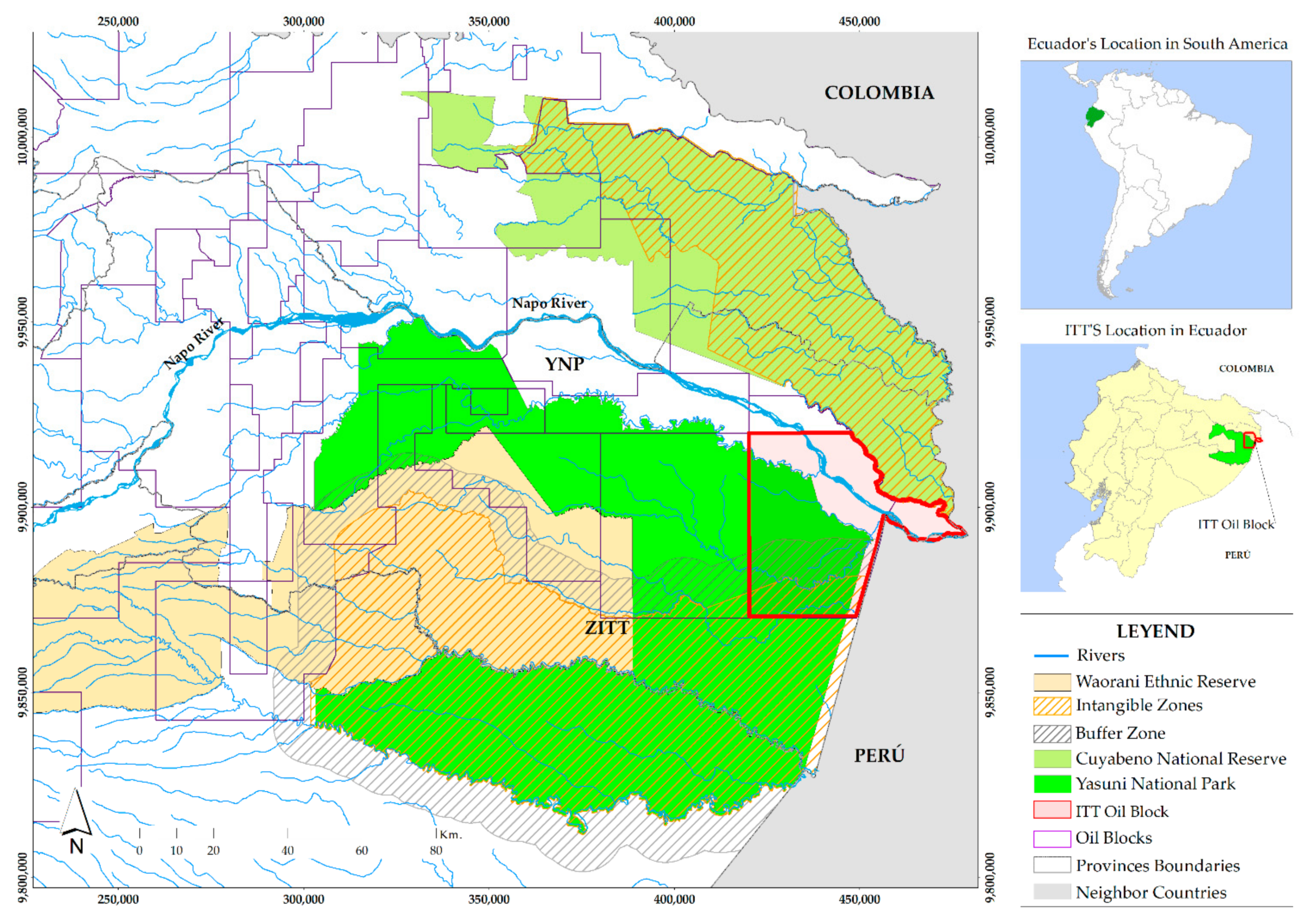
The study took place in the ITT Oil Block (Ishpingo, Tambococha, and Tiputini), also called Block 43 [62], which is in the Province of Orellana (Aguarico canton), covering an area of 179,449.53 ha. The Ishpingo and Tambococha fields are within the YNP, while Tiputini is outside of it. The limits of the ITT Oil Block are the Cuyabeno Wildlife Reserve to the north, ZITT to the south, the Peruvian border to the east, and the YNP to the west (Figure 1) [63]. This area comprises lowlands and gently sloping plains covered with sediments of fluvial and lake origin, as well as medium hills, high terraces, and a low river level that in turn belongs to the lower basin of the Napo River and its sub-basins; therefore, the canton remains flooded during bouts of high rainfall.

The ecosystems that exist are the Aguarico-Putumayo-Caquetá lowland evergreen forest, the Amazon (Pantano) flooded forest with palms and alluvial plains, the floodplain forest of alluvial plains with rivers of Andean and Amazonian Cordillera origin, and the Amazon-flooded lake-riparian grassland of alluvial plains [64,65]. Their climate is very tropically humid with altitudes of 65 to 600 m above sea level, an average annual temperatures of between 24 °C and 27 °C, and high annual rainfall (3200 mm to 6315 mm and high annual relative humidity (80–94%) [53]. According to the United States Department of Agriculture’s (USDA) classification, the soil orders are as follows: Entisol in 60,857.8 ha (5%), Base Wn in 14,918 ha (1%), and Inceptisol in 11,042,002 ha (93%) [66]. The population of the Aguarico canton is 4847 inhabitants (7.1%) out of a total of 136,396 inhabitants who dwell in the province of Orellana. The households in Aguarico number around 3044 [67].

The ITT Oil Block is superimposed on the landscape of two protected areas, namely the YNP and Cuyabeno Wildlife Reserve, and presents abundant biodiversity with 191 species of mammals, representing 16.23% of species registered in the eastern tropical floor. Regarding birds, it is home to 25 families belonging to 13 orders, which represents 700 species (6% of all those in the Amazon) and some 2.59% of Ecuador’s continental species. There are also four recorded species of reptiles (3.08%), 17 species of amphibians (11.11%), and a high number of insect species [68].

2.2. Method

Multitemporal analysis is defined as the detection of changes in coverage between two different dates by deducing the evolution of the natural environment or the incidence through anthropic action on it [69]. It was performed by interpreting information from remote sensors by considering satellite images and determining the interpreted units and images of the results [70]. There are several studies in the Ecuadorian Amazon region concerning the implementation, monitoring, and detection of environmental changes with remote sensors, such as in the area of changes in land cover in the fluvial geomorphology of the Tena River [71], and in land use regarding carbon storage in productive systems and primary forests [72]. The change of land cover and use is a dynamic process of expropriation on the ground, related to anthropic activities (livestock, agriculture, etc.) [73]. The change is visible in high parts of mountains, hydrographic basins, and areas adjacent to rivers and streams, which are increasingly larger and occur rapidly, causing loss of forest cover, and a decrease in the quantity and quality of water and soil, thereby affecting communities who reside in the basins [74]. It is a conditioner of different types of movements and has an important influence on the hydrological and mechanical properties of the soil [75].

The detection of changes in soil dynamics is monitored by means of satellite images of the area. The change occurs due to various natural factors, such as anthropic ones. A multitemporal study assesses the changes in vegetation cover that existed in the area with the interpretation of satellite images, for instance Landsat, Sentinel 2A, and Spot [76]. Remote sensors gather information from the study area that is physically far from the sensor equipment (satellites or airplanes) that will later be analyzed [77,78]. In the ARE, there are some case studies where remote sensors were applied, such as in the area of deforestation [9], agrarian reforms [79], changes in land use in agricultural-forest landscapes [70], and forest fragmentation [80].

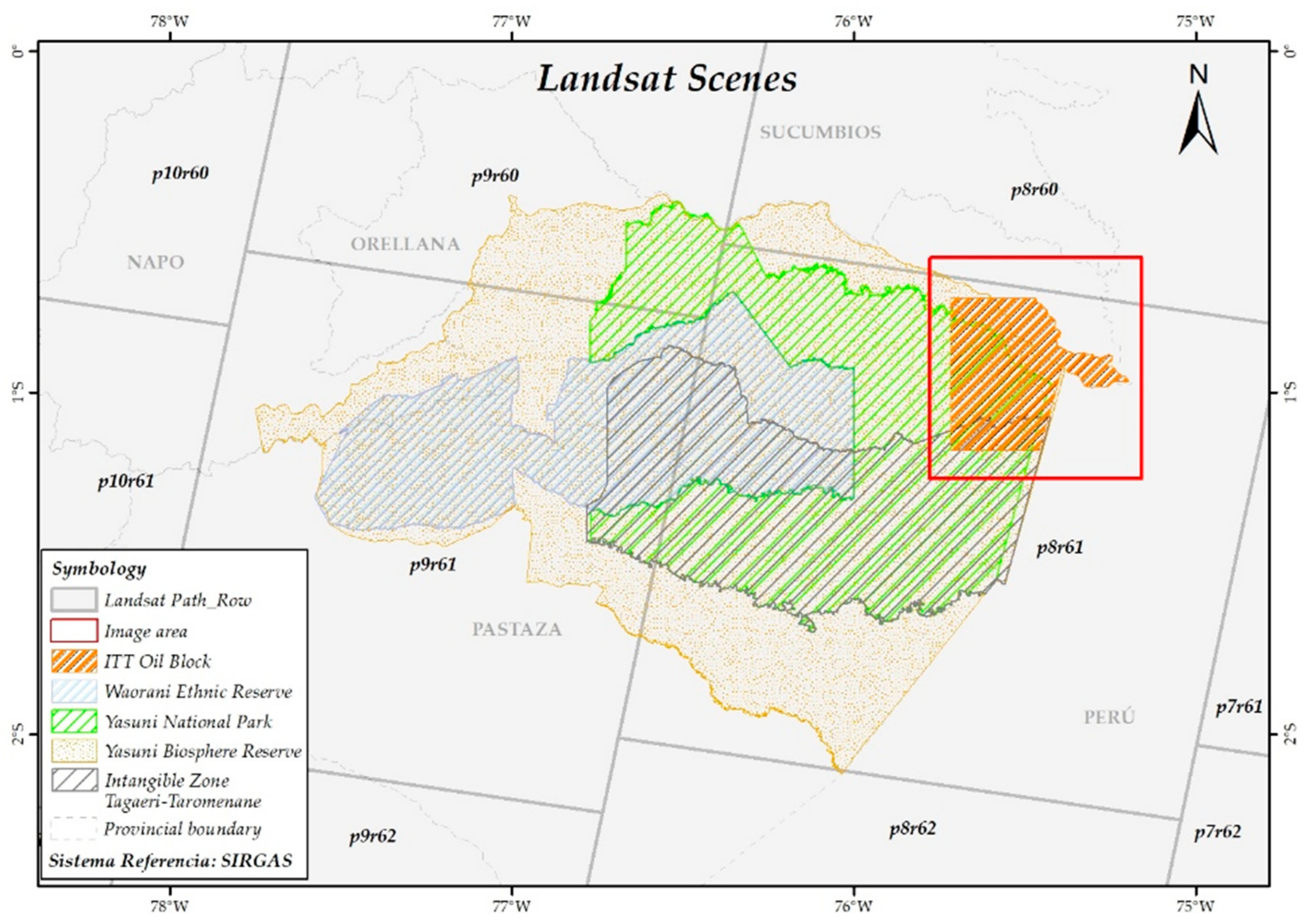
Landsat 7 and 8 satellite images were used because it is the sensor with the greatest application in territorial studies, which includes agriculture, forestry, land use, hydrology, and environmental monitoring [81] (Figure 2). Bands were combined because the spectral range combination means that each band of the satellite image allows one to highlight the characteristics of the area of interest [82]. For example, to highlight the vegetation of a satellite image, the Infrared combination of bands 5 4 3 (Landsat 8) or 4 2 1 (Landsat 7) needed to be conducted.

Unsupervised classification was used because it is a clustering tool that allows subgroups called clusters within a group and classifies the elements of this group based on the similarity between them [83]. The Normalized Difference Vegetation Index (NDVI) was also used, which is a non-dimensional index that allowed us to measure the relationship between the energy absorbed and emitted from terrestrial objects that, when applied to a group of plants, yield values of intensity concerning greenery and the amount of vegetation present in the area as well as its vegetative state ranging from −1 (not forest) to +1 (forest) [84]. Likewise, the raster, calculator raster, and crosstab were used [85,86].

The PCI Geomatic software was used, which processes satellite images from all aerospace platforms (multitemporal analysis) [87], and has two levels: Geomatica core (which classifies satellite images) and Geomatica prime (which has analytical geoprocessing functions). It is also compatible with the ARCGIS software [Carbonnel and Quijada, 2018], which collects, organizes, manages, analyzes, shares, and distributes geographic information [88].

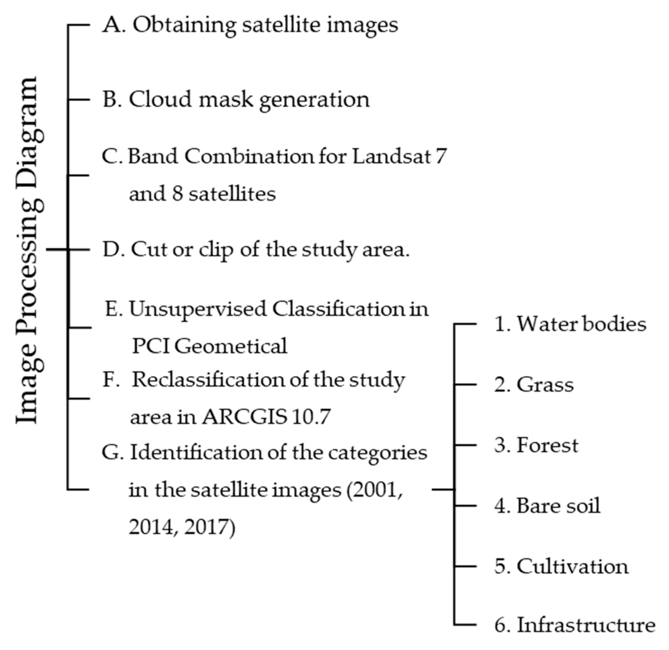
The current study had four main specific objectives: To classify the images from the years 2001, 2014, and 2017; identify existing types of land cover; to quantify changes in land use in the ITT Oil Block of the Amazon; and to characterize the factors associated with the change in land use of the ITT Oil Block. For the fulfillment of these objectives, individual methodological processes were implemented. However, for the first three objectives, the activities in the satellite image processing flow diagram were performed for the three periods (Figure 3).

2.2.1. Identification of the Categories in the Satellite Images (2001, 2014, 2017)

(a)

Satellite Images

For the analysis of changes in land use, Landsat 7 was used for the year 2001, while Landsat 8 was used for 2014 and 2017 with a spatial resolution of 30 × 30 m and a percentage of cloud cover of less than 30%. These were downloaded from the United States Geological Survey (USGS) platform. This format contains all the image bands to make the band combinations.

The downloaded images are of the “L1T” type, thus they have geometric corrections based on control points and digital terrain models [89], with the UTM coordinate system and WGS-84 reference system in Zone 18 South. The images were processed using the PCI Geomatical application and ARCGIS 10.7.

The Landsat 8 satellite images for 2018 and 2019 presented a large percentage of cloud cover in the study area. When making cloud layers of the 2019 image, a cut was visualized in the entire northern part of the area of interest, which did not allow a complete analysis of the image so it was replaced by another Landsat 8 image from 2017.

Meanwhile, the Landsat 7 satellite platform presented radiometric and geometric errors on the lateral sides of the images as of 2002, so we worked with the image of the last date in 2001 since it does not have these errors and presents a lower percentage cloudiness in the area of interest.

(b)

Cloud mask generation of the satellite images of the different periods

During the analysis of the study area, the satellite images presented clouds, thereby altering the results, so masks of the clouds were realized in the three images of the different periods, giving values of 1 and 0 to the clouds and creating a new raster for combining bands in order for the clouds to be considered a single pixel value [82].

For the creation of cloud masks, the ARCGIS 10.7 program was used, with the bands 2, 3, 4, 5, 6, and 7 of the Landsat 8 satellite image in 2017 (Raster) and the shapefile (Vector) of the study area (ITT Oil Block) in order to locate the area of interest in the generated raster. If clouds were present, a mask of clouds (Mask Cloud) of the period was created. We added the BQA band (band of evaluation or quality control) that has the decimal value of pixels for the clouds.

The Raster Calculator analytical tool was triggered to execute the CON condition (controls the output value for each pixel based on whether the pixel value evaluates to true or false on a specific conditional statement) and the BQA band was added for the purpose of changing the pixel values of the clouds to 0 and 1 with the following algebraic expression:

CON (Band BQA > = Decimal value of the cloud, 0, 1).

(1)

Then the Raster Calculator was used but with the FLOAT condition (converts the value of each raster pixel into a floating-point representation) and the multiplication of the two bands, with band 2 of the satellite image and the Cloud Mask, with the following equation:

FLOAT (“Band 2 (Blue)” * “Cloud Mask”).

(2)

The final step of the cloud layer generation process was to save this new raster in the same location as the other Landsat 8 bands of the period with the name “Band 2_cloud”.

(c)

Process for cutting the study area (ITT Oil Block) from the satellite images in PCI Geomatics

A section was generated of the study area of all the bands of the satellite image for the three periods in order to reduce the processing time of the images when classifying in the PCI Geometics program [82]. Hereby, the PCI Geomatics program was run in its trial version (https://www.pcigeomatics.com/resources/more-resources/downloads; accessed date: 24 January 2021) to generate a base meta in a PIX format, adding the bands of the image of the period to be worked on in the layers panel. Then the File option was selected from the menu bar, which displays a list where the Utility option was chosen and then the Import to PCIDSK option. A window opened that gives the options to select the file to import and the destination to save that file. In this case, band 2 (blue) of the Landsat 8 image was selected and saved in the same location as the bands studied.

The same process was conducted again, but instead of selecting the import to the PCIDSK option, ‘Transfer layers’ was selected to transfer layers from one file to another. In this case, all the utility bands were selected for the analysis, including the new raster generated in the ARCGIS program (“Band 2_cloud”) and the transfer option was chosen. After completing the transfer of layers to the new base meta in a PIX format, we selected ‘File’ from the menu bar and ‘open’ to open the new base meta generated in the previous process.

The satellite images were cut for the study area using the option ‘Clipping/Subsetting’ in the Tools menu, which opened a window requesting the base goal to perform this action; in this case, the file generated in P2 was chosen. Then the cutting method was selected and ‘Selection to Clip Layer’ was chosen. The shapefile of the area of interest (ITT Oil Block) was inserted. Finally, the destination to save this cut with the bands and Clip was chosen and a new base meta was generated called “L8_ITT_2017.pix”.

(d)

Unsupervised Classification Process in PCI Geomatics

The new file generated in the previous process (L8_ITT_2017.pix) was opened with the bands cut from the study area. A new raster was created within the base “L8_ITT_2017.pix” with 32 bits real-time format. When generating this new raster called “CNSITT2017”, the unsupervised classification was performed from the Analysis, Image Classification, and Unsupervised options.

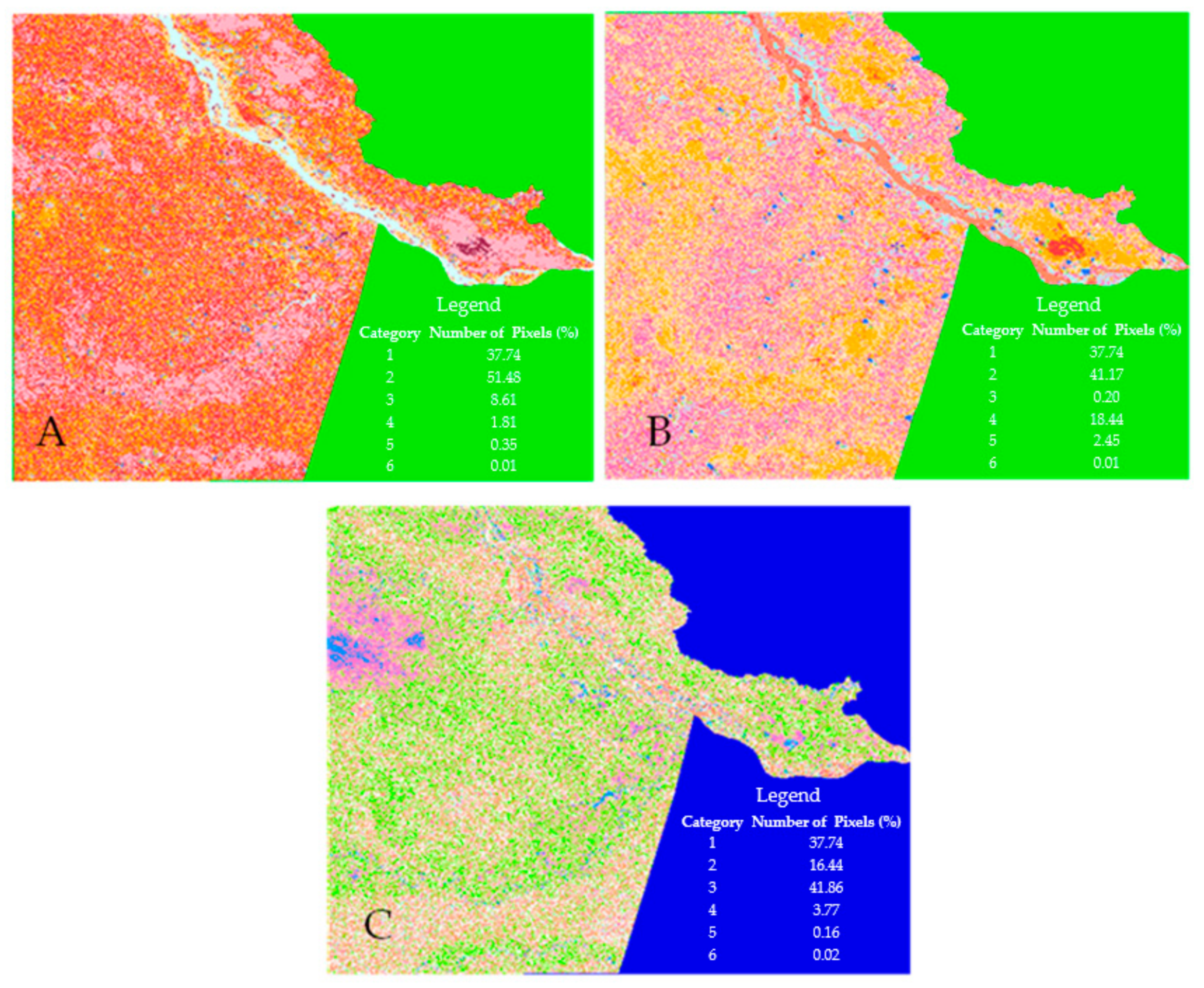
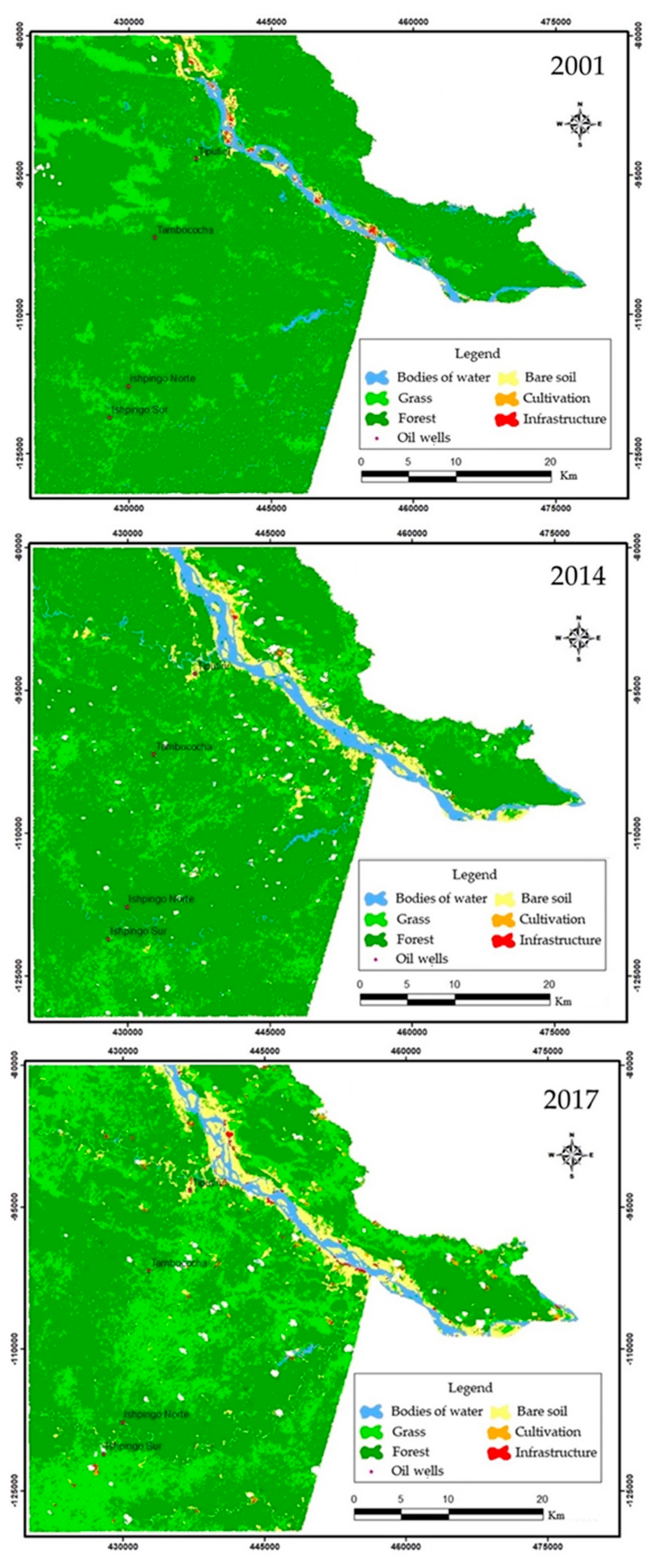
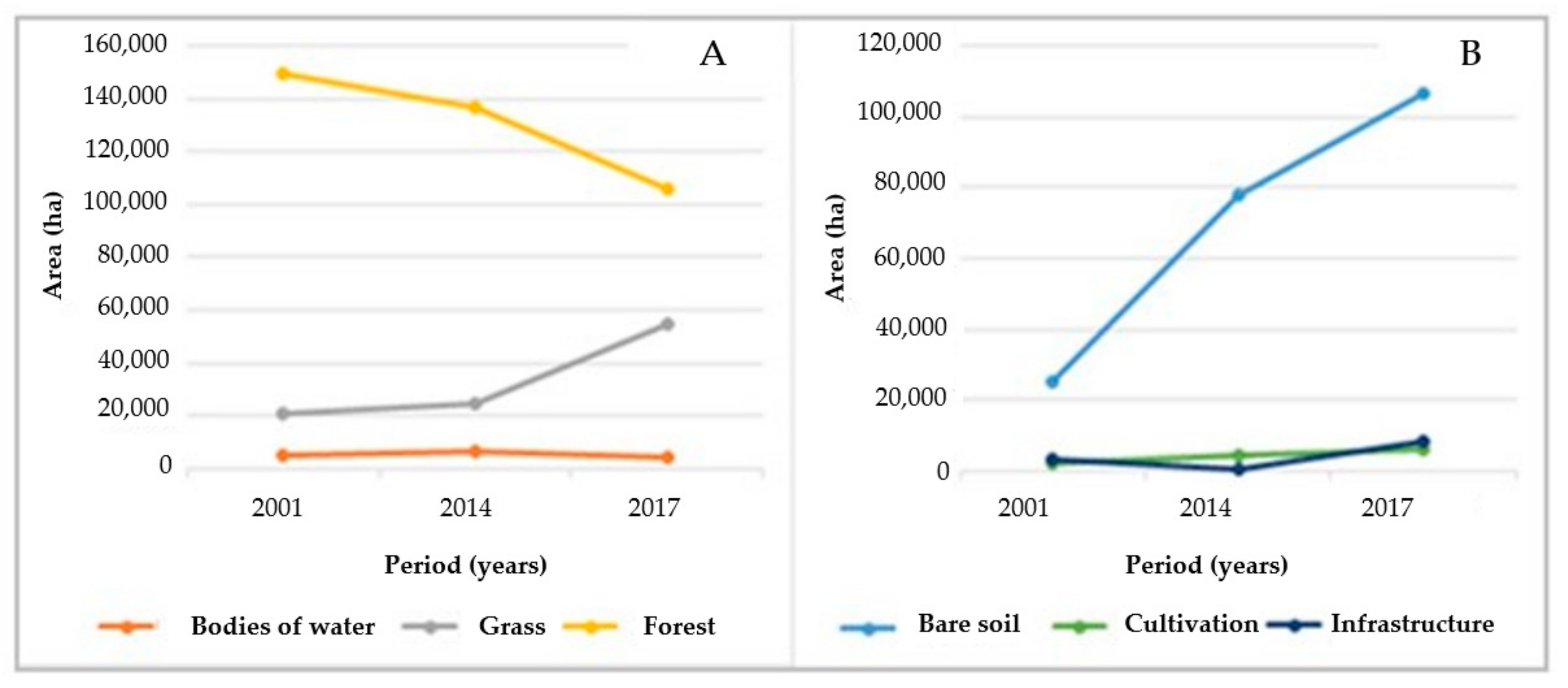
From a combination of bands (2, 5, 6), the unsupervised classification was generated where it was evidenced that categories 1 and 2 have the highest amounts of pixels for 2001 and 2014, while for 2017 it was category 1 and 3 (

Table 1. Information on the unsupervised classification in PCI Geomatics for the years 2001, 2014, and 2017 in the ITT Oil Block of the Ecuadorian Amazon region.

2001			2014		2017
Category	Number of Pixels	% Pixels	Number of Pixels	% Pixels	Number of Pixels	% Pixels
1	1,208,527	37.74	1,208,527	37.74	1,208,527	37.74
2	1,648,690	51.48	1,318,273	41.17	526,605	16.44
3	275,615	8.61	6473	0.20	1,340,573	41.86
4	57,896	1.81	590,469	18.44	120,889	3.77
5	11,293	0.35	78,382	2.45	5240	0.16
6	337	0.01	234	0.01	524	0.02
Total	3,202,358	100	3,202,358	100	3,202,358	100

; Figure 4).

A new window was opened that requests the number of classes and a maximum of classifiers. In this project, 24 classes were applied with a maximum of 24 classifiers, considering that for every four pixels, they present similar digital values and we multiplied by the six predefined classes for this area.

Then the selection of bands to be combined and the band to be classified was requested, in this case the following bands were used: B2_clouds (cloud layer), Band 5, and Band 7. For the classification, we used “CNSITT2017” and clicked accept. The unsupervised classification was generated in the “CNSITT2017” raster, which was exported in another PCIDSK (PCI Geomatics Database File) by right-clicking on the classified raster and clicking save/export. It was saved in a new PCIDSK named CNSITT2017.pix with the transfer of the band or raster “CNSITT2017.Tiff”.

2.2.2. Identification of the Types of Land Cover in Each of the Zones

While obtaining the raster file of the three periods, six categories were identified, namely bodies of water, grassland, forest, bare soil, cultivation, and infrastructure [82]. The bodies of water were categorized by the presence of the Napo river basin and the sub-basins (Aguarico, Nashiño, Yasuní, Tiputini, and Cononaco) [90] in the Aguarico canton where the Tiputini river is located. The grassland was defined based on the use and coverage of the soil. Forest cover was witnessed in the satellite images and because the area has some ecosystems. Bare soil was assigned to roads, non-forest areas, and rock formations. The cultivation was categorized due to the use of the land in the Aguarico canton. Infrastructure was defined as everything that is buildings, homes, platforms, and oil wells (

Table 2. Land use and land cover classification scheme in the ITT Oil Block of the Ecuadorian Amazon region.

Categories	Description	Example of Aerial View
Bodies of water	The bodies of water were categorized by the presence of the Napo River basin and the sub-basins (Aguarico, Nashiño, Yasuní, Tiputini, and Cononaco) in the Aguarico canton where the Tiputini river is located.
Grassland	This refers to areas that are not considered agricultural areas. It also includes areas where the vegetation structure does not meet the definition of forest land and is expected to remain so without human intervention.
Forest	A group of trees with a minimum canopy coverage of 30%, an upper layer height of at least 5 m and a minimum area of 10,000 m2 (1 ha).
Bare soil	Bare soil was assigned to roads, non-forest areas, and rock formations.
Cultivation	Areas under cultivation, such as monocultures and agroforestry systems where the vegetation structure does not meet the definition of forest land.
Infrastructure	Infrastructure was defined as houses, other buildings, platforms, and oil wells.

) [91].

Thus, in the procedure for the reclassification of the ITT from the different periods, the ARCGIS 10.7 program was opened for the reclassification of the new PIX file. For this, the CNSITT2017.pix file was added. For the reclassification of the raster file, reclassify (ArcToolbox/Spatial Analyst Tools/Reclass) was executed. A new window was opened requesting the raster to apply the action, then the classify option was enabled to choose several classification options and the number of classes. In this project, we used equal intervals with six classes. Everything was accepted and the tool was executed.

A new reclassified raster was generated that modifies the colors for each class (Gridcode) depending on the classes proposed for the analysis of this project. Once the classification was made, the Raster to Polygon tool (ArcTollbox/Conversion Tools/From Raster) was executed, allowing us to transform the Raster generated by the reclassification into a polygon (Vector) to perform the area calculation. Once the polygon of the classified study area was generated, the area was calculated. For this, the polygon’s attribute table was opened and in the new window that appeared, the Add Field option was chosen, which created a new column previously configured to perform the calculation of their areas in hectares (ha). After this, we right-clicked on the new column and the Calculate Geometry option was selected to obtain the areas in ha.

Polygons with a smaller area were eliminated because there are pixels or errors in the raster image and also because they are not visible on the map and can alter the analysis of the results. In this project, polygons of areas smaller than 2 ha were eliminated using the Eliminate tool (ArcToolbox/Data Management Tools/Generalization). A new polygon was generated, with areas smaller than 2 ha removed, therefore its properties were opened and in Symbology we chose Show/Categories panel and in the Value field, “Gridcode” was selected and all the values were added (Add all values). A list of the classes and colors was generated. As an extensive classification among the six classes was generated in P3, and the Dissolve tool was run to reclassify these pixels by their gridcode.

Prior to performing the Dissolve action, some steps needed to be considered. As the classification was generated, the attribute table of the last generated polygon was opened and another column named Dissolve was added. Then, it was selected by attribute. In this case, the Gridcodes of the same color were chosen by means of the expression (Gridcode = the value of the Gridcode of the class) or if there were more classes with the same color, the “OR” condition was added as in this expression (Gridcode = value of the Gridcode of the OR class Gridcode = value of the Gridcode of another OR class) and the amount of Gridcode that belongs to the same class. Later in the attribute table, we clicked on the Dissolve column and the Field Calculator option was selected. A window appeared with a text space at the end that requests the value of this class. In this project there are six classes, so the Gridcodes to be analyzed were given values from 1 to 6 and the unclassified ones (No data) were given values of 0. Finally, after completing the previous step, the Dissolve tool (ArcToolbox/Data Management Tools/Generalization) was executed, generating a new polygon, but this time with six categories in the attribute table, consisting of the area calculation and the modification of the colors for each category.

All these procedures were applied, for the 3 satellite images in the years 2001, 2014, and 2017 in the study area.

2.2.3. Quantification of Land-Use Changes in the ITT Oil Block of the Amazon

(a)

Crosstab

This methodology was applied in order to calculate the difference between the categories of the different periods. That is, the loss or increase in area in hectares of each category was calculated over the years using the ARCGIS 10.7 program with the Tabulate Area tool (ArcToolbox/Spatial Analyst Tools/Zonal). It automatically generated a matrix of the areas of each category in hectares for the three periods [82].

(b)

Estimation of the Annual Average Deforestation Rate (AADR)

For the calculation of the annual average of the loss of forest surface between two determined times, the annual average rate of deforestation was applied (Equation (3)) using hectare per year (ha/year) as the unit measurement. The AADR equation is the average annual rate of deforestation:

$$AAD{R}_{jt1-t2}=\frac{\left(A{B}_{jt1}-A{B}_{jt2}\right)}{n}$$

(3)

where:

t₁ is the initial year and t2 is the final year.

AADR_jt1–jt2 is the average annual rate of deforestation and j is the moment (t1 and t2).

AB_jt1 is the area covered by forest in the first period.

AB_jt2 is the area covered by forest in the second period.

n is the difference of years between both periods.

(a)

Estimation of the change rate of land cover and use

The calculation of the rate of change of land cover and use was performed by applying the equation proposed by Puyravaud [92], implemented by Sucoshañay and Corral, (2016).

$$r=\frac{1}{\left(t_2-t_1\right)} \ast ln\frac{A2}{A1}\ast \left(100\right).$$

(4)

where:

r is the annual rate of change of land cover and use.

A1 is the land-use area in the first period.

A2 is the land-use area in the final period.

t₁ is the initial period.

t₂ is the final period.

2.2.4. Soil Parameters in ITT Oil Block

The historical relationship between the periods (2001–2017) was analyzed through a bibliographic review, where those biophysical, demographic, socioeconomic, political, and environmental aspects that have directly or indirectly affected the ITT Oil Block over time are studied.

For the characterization of the factors associated with the change in the use of soil in an ecosystem sensitive to industrial use, secondary information was used, such as a physical-chemical analysis of the soil conducted in the Tiputini and Tambococha platform area by the public company Petroamazonas in 2011, where the parameters Total Hydrocarbons (TPH), Polycyclic Aromatic Hydrocarbons (HAPAs), Cadmium (Cd), Nickel (Ni), and Lead (Pb) were analyzed in order to verify the permissible limits for sensitive ecosystems (Reglamento Ambiental de Operaciones Hidrocarburíferas, 2020).

Table 3. Permissible soil limits in the ITT Oil Block of the Ecuadorian Amazon region.

Parameter	Unit	Sensitive Ecosystem	Industrial Use
TPH	mg/kg	<1000	<4000
HAPs	mg/kg	<1	<5
Cd	mg/kg	<1	<10
Ni	mg/kg	<40	<100
Pb	mg/kg	<80	<500

indicates detailed permissible limits of the Tambococha soil [93].

3. Results and Discussion

3.1. Unsupervised Classification of the ITT Oil Block

The classification of the images was unsupervised because the study area is militarized and it is forbidden to fly aircraft and drones over it. The unsupervised classification was performed with the PCI Geomatics tool based on Melo [94]. Hereby, we compared the processing performance and classification of images between ARCGIS 10.7 and PCI Geomatica. The latter turned out to be better in runtime, image loading time, display, intermediate process time, etc. It was concluded that it is faster and more efficient, and the classification process was compared to ARCGIS 10.7. In another multitemporal study [83] on fire recurrence areas that was conducted in the Metropolitan District of Quito, they recommended the application of this methodology for the treatment of satellite images that is of importance for analysis and the geometric and radiometric corrections of the image need to be considered previously. Subsequently, they applied unsupervised classification for the respective digitization.

3.2. Identification of the Types of Land Cover in Each of the Zones

For the analysis of changes in land use, six categories were identified: Bodies of water, grassland, forest, bare soil, cultivation, and infrastructure. In the classification of the 2001 period, the forest category presented the highest number of pixels, followed by grassland and bodies of water. Those with the least number of pixels were cultivation, soil, and infrastructure. The latter was visualized in the surroundings of the bodies of water category and we observed large forest cover in the ITT Oil Block (Figure 5).

For the classification of the 2014 period, the forest category presented the highest number of pixels, followed by grassland, soil, and bodies of water. Those with the least number of pixels were cultivation and infrastructure. An extension of soil was visualized on the shores of the body of water in the ITT Oil Block and a lower amount of infrastructure than in the previous period (Figure 5 center). For the classification of the 2017 period, the grassland category presented the highest number of pixels, followed by forest, soil, and bodies of water. Those with the least number of pixels were cultivation and infrastructure. It was visualized that the soil category had expanded with respect to the two previous periods and that the forest category decreased enormously (Figure 5 lower part).

In a similar study conducted in the south of the Napo province, in the Tena canton, on the banks of the Napo river, the following units were defined, being forest, urbanized areas, agricultural mosaic (coverage made up of associations between different types of crops), predominance of pastures and crops (areas of predominance of grass-type species and short-cycle crops), and bodies of water [70].

3.3. Quantification of Land-Use Changes in the ITT Oil Block of the Amazon

The changes in land use in the ITT of the Ecuadorian Amazon in the three periods were quantified using the Cross Tabulation methodology (

Table 4. Area in hectares for each category in the ITT Oil Block of the three periods.

Periods	2001		2014		2017		Total
Categories	Ha	%	Ha	%	Ha	%	(2001–2017)	%
Bodies of water	5379.38	2.99	6329.97	3.53	4379.39	2.44	999.99	0.56
Grass	20,917.34	11.66	24,530.50	13.67	55,064.2	30.69	−34,146.89	−19.03
Forest	149,330.20	83.22	137,157	76.43	105,847	58.98	43,483.47	24.23
Bare soil	2515.26	1.40	779,661	4.35	10,640.80	5.93	−8125.56	−4.53
Cultivation	184.66	0.103	427.68	0.238	591.29	0.33	−406.63	−0.23
Infrastructure	311.69	0.174	54.81	0.031	803.85	0.448	−492.16	−0.27

). In 2001, the forest area (primary and secondary) covered 149,330.16 ha (83.22%) of the 179,449.53 ha of the total area of the ITT area. Bare sole in the ITT made up 2515.26 ha (1.40%) and agriculture made up 184.66 ha (0.10%). By 2014, the forest had decreased to 137,157.12 ha (76.43%), while bare soil increased to 7796.61 ha (4.34%), as did cultivation to 427.68 ha (0.24%). By the third period (2017), the forest had decreased to 105,846.69 ha (58.98%), whereas bare soil increased to 10,640.82 ha (5.93%) and cultivation to 591.29 ha (0.33%) (Figure 6).

Upon comparing the years 2001 and 2017 in the ITT Oil Block, it is clear that over the 16 years there were greater changes in land use within bodies of water as it lost 0.56% (999.99 ha). Meanwhile, pasture increased by 19.03% (34,146.89 ha), forests decreased by 24.23% (43,483.47 ha), soil increased by 4.53% (8,125.56 ha), and cultivation increased by 0.23% (406.63 ha). This is due to the fact that infrastructure increased in the area, occupying 0.27% (803.85 ha) in 2017 (Table 4).

This quantification of hectares for each category was taken as a reference for the image of the year 2001, which served as the basis for calculating the annual average rate of deforestation and rate of changes in land cover and use in the other two years of interest.

Furthermore, Equation (3) was applied in order to analyze the average annual deforestation rate in the ITT Oil Block for the 2014 and 2017 periods in the Ecuadorian Amazon, taking the 2001 period as the basis of analysis. Thus, the deforestation rate for the period 2001–2014 was calculated, which was 936.39 ha/year (5). This is equivalent to 0.63% compared to the original forest that existed in the 2001 period (

Table 5. Deforestation rate in the ITT Oil Block of the Ecuadorian Amazon region.

Period	Annual Deforestation Rate (ha/Year)/(%)
2001–2014	936.39 (0.627)
2001–2017	2717.71 (1.82)

).

$$AAD{R}_{\left(2001–2014\right)}=\frac{\left(A{B}_{\left(2001\right)}-A{B}_{\left(2014\right)}\right)}{n}$$

(5)

$$AAD{R}_{\left(2001–2014\right)}=\frac{\left(\mathrm{149,330.16}-\mathrm{137,157.12}\right)}{13}$$

$$AAD{R}_{\left(2001–2014\right)}=936.39 \mathrm{ha}/\mathrm{year}.$$

The deforestation rate for the period 2001–2017 was calculated at 2717.71 ha/year (6), which is equivalent to 1.82% with respect to the original forest that existed in the 2001 period (Table 5).

$$AAD{R}_{\left(2001–2017\right)}=\frac{\left(A{B}_{\left(2001\right)}-A{B}_{\left(2017\right)}\right)}{n}$$

(6)

$$AAD{R}_{\left(2001–2017\right)}=\frac{\left(\mathrm{149,330.16}-\mathrm{105,846.69}\right)}{16}$$

$$AAD{R}_{\left(2001–2017\right)}=2717.71 \mathrm{ha}/\mathrm{year}.$$

3.4. Characterization of the Factors Associated with the Change in Land Use of the ITT Oil Block

The rate of land cover and use changes in the ITT Oil Block was calculated using Equation (4), based on the anthropogenic activities that existed in the ITT Oil Block. In the years 2001, 2014, and 2017, the results determined that land use tended to decrease the vegetation cover. In other words, the deforestation rate of the ITT Oil Block, located in the upper part, was 2.15%. The worst affected zones were those in the vicinity of the populated areas and the Napo River Basin. During the period studied, cultivation had the second-highest rate of change at 7.27%. In terms of extension, bare soil is the most representative in the ITT Oil Block with a percentage of 9.01% (

Table 6. Annual rate of change of land cover and use in the ITT Oil Block of the Ecuadorian Amazon region for the period 2001–2017.

Categories	2001	2017	Land-Use Change Rate (ha)/(%)
Bodies of the water	5379.38	4379.39	−0.01/−1.29
Grass	20,917.34	55,064.23	0.06/6.05
Forest	149,330.16	105,846.69	−0.02/−2.15
Bare soil	2515.26	10,640.82	0.09/9.01
Cultivation	184.66	591.29	0.07/7.27
Infrastructure	311.69	803.85	0.06/5.92

).

In a similar study carried out in the Puyo River Basin in the Ecuadorian Amazon, the same equation was implemented [92]. The results of that research between the periods 2000, 2004, and 2013 were that land use has a tendency to decrease forest cover (the deforestation rate was 4%), especially in areas close to mountains. Moreover, the increase in cultivation near rural areas (4%) showed the productive evolution of the study area. In addition, the increase in areas without vegetation cover and populated areas was evident [95].

3.5. Soil Parameters in ITT Oil Block

A bibliographic review was performed in order to understand the incidents on each of the categories that were analyzed in the ITT Oil Block during the three given periods. In 2001, the bodies of water category represented 2.99% (5379.38 ha), but in 2014, it increased to 3.52% (6329.97 ha). This occurred due to several aspects, such as the movement of streams and the increase in flow and erosion along the banks [96]. Regarding infrastructure, in 2001 it had a surface area of 0.174% (311.69 ha) and there were some homes near the Napo River, but in 2014 it decreased, occupying 0.031% (311.69 ha). This happened due to the high rainfall in the Province of Orellana, which generated flooding along the Napo River, and as its water storage capacity was saturated in the middle basin, causing floods (greater than 5000 m³/s) on 6 April 2010 [97]. The changes in land use in the ARE occurred due to the implementation of public policies to control and access Amazonian spaces, the extraction of natural resources, and agriculture [98].

Deforestation and changes in land use occur due to human activities such as agriculture, livestock, and human settlements [99]. According to INEC [67], the number of inhabitants in the Aguarico canton in 2001 was 4658, whereas in 2010 it was 4847, that is, it increased by 0.42%, which means that the population expanded throughout the Amazon basin, decreasing the forest cover of the area to 105,847 ha, 58.98% of what it had been in 2001 (149,330.2 ha). In a study conducted in the northern Ecuadorian Amazon, which covers the Sucumbíos, Orellana, and Napo provinces, deforestation was caused by two reasons, the discovery of oil and construction of ballasted and unburdened roads to transport oil by pipelines to Esmeraldas (the Pacific coast) for export, and secondly the migration of rural populations from the Sierra region caused by the need for land [100]. In the 1960s, oil reserves were discovered in the northern Ecuadorian Amazon, which accelerated the processes of colonization of new areas in the lowlands [37]. Previous studies demonstrated that the activities generated by the oil companies and the construction of roads were the main causes because they promoted deforestation and agricultural settlements in the ARE [68].

The strongest dynamics of land-use changes between 2001 and 2017 was concentrated along the banks of the Napo and Yasuní rivers. This probably occurred due to the urban population growth in Tiputini and Rocafuerte [101]. The intensification of agricultural activities that existed in the ITT Oil Block was reflected in 2014, occupying an area of 427.68 ha, which represents 0.23% of the ITT Oil Block. In 2017, it increased to 591.29 ha (0.329%). This is due to small farm producers, who incorporate the forested area into agricultural production, thus becoming the main factor in deforestation and degradation in the area [102].

With respect to the physical-chemical analysis of the soil performed in 2011 and 2015 in the Tiputini and Tambococha platform area, it was evidenced that the following parameters were way above the limits allowed by Ecuadorian legislation in the Tambococha area: The TPH, Cd, and Pb in 2011, and TPH, HAPs, and Pb in 2015. TPH, HAPs, and Cd also exceeded permissible limits in Tiputini in 2015 (

Table 7. Results of the physical-chemical analysis in the Tambococha area. The first results are from EIA and PMA (code B1), the second from ACT. EIA and PMA (code B1), and soil quality criteria are from AM 097 -A (Table 1) [103], based on the Environmental Impact Study 2011 [104] and Update on the Environmental Impact Study Project Development and Production of the Tiputini and Tambococha Fields 2015 [105].

Parameter	Unit	2011 Result	2015 Result	Soil Quality Criterium	Observation
TPH	mg/kg	1470	<100	<150	Fails
HAPs	mg/kg	0.053	<0.364	0.1	Complies in 2011
					Does not comply in 2015
Cd	mg/kg	<2	<0.500	0.5	Does not comply in 2011
					Complies in 2015
Ni	mg/kg	3	<10.0	19	Complies
Pb	mg/kg	78	13.5	19	Does not comply in 2011
					Complies in 2015

and

Table 8. Results of the physical-chemical analysis of the Tiputini area. The first results are from EIA and PMA (code B1) and soil quality criteria are from AM097 -A (Table 1) [103], based on the Environmental Impact Study 2011 [104] and Update on the Environmental Impact Study Project Development and Production of the Tiputini and Tambococh Fields [105].

Parameter	Unit	2011 Result	Soil Quality Criteria	Observation
TPH	mg/kg	3801	<150	Fails
HAPs	mg/kg	0.11	0.1	Fails
Cd	mg/kg	<2	0.5	Fails
Ni	mg/kg	2	19	Complies
Pb	mg/kg	<9	19	Complies

). If environmental measures are not applied that allow people to prevent, avoid, and control the use of land, the sensitive ecosystem will change to ‘industrial land use’, thereby losing the existing biodiversity in the area, such as species like Podocnemis expansa, which is in a critical condition, hence it is on Ecuador’s red list.

3.6. Possible Political Implications for Restoration and Planning in the ITT Oil Block of the Ecuadorian Amazon Region

Local and regional entities should promote projects to improve human well-being and the restoration of ecosystems in the ITT Oil Block using 4% of the funds of the sale price for each oil barrel. This has been arranged to invest in the areas of influence of oil, mining, and electricity exploitation projects according to the Organic Law for the Integral Planning of the Amazon, Special Territorial Circumscription [106]. This law, approved by the National Assembly of Ecuador and published in the Official Register Supplement 245 on 21 May 2018, is fundamental for administrative and environmental legislation, as it seeks to increase and diversify production, promote technology transfer, strengthen comprehensive security, and generate opportunities in the Amazon region [107].

It is essential to seek an unprecedented global governance mechanism that promotes environmental justice and is an innovative development proposal. Oil extraction is a useful perspective to think and write about in regards to the future of the use of resources, which seeks to achieve the sustainability of the Ecuadorian Amazon region.

Considering the global importance of the RBY and the Amazon basin in terms of conserving its high diversity, the findings of this research contribute to reformulating a governance model for the ITT oil block, similar to the one carried out for the Diversity and Life Zone, which has been established by national and local organizations public organizations [108] that aim to (a) strengthen governance; (b) achieve a balance between the conservation of the environment and living conditions; and (c) rescue cultural dynamics. A new management model for the ITT oil block would be implemented through a special regime that guarantees sustainability and minimizes risk factors for indigenous communities and migrant settlers, with greater emphasis on biodiversity [109].

4. Conclusions

The unsupervised classification of the images allowed the visualization of variations of vegetation cover, hydrographic basins, and soils of the ITT Oil Block of the Ecuadorian Amazon through the automatic use of tools, such as PCI Geomatic and ARCGIS without the need to visit the study area. In the current investigation, as it is an area of national interest, certain areas cannot be accessed and flying objects (drones and airplanes) are prohibited in the area, so satellite images from the periods of 2001, 2014, and 2017 were used.

The study area was classified into six categories, where the infrastructure was identified by geometric shapes and colors that have a group of pixels of the same values, while agricultural lands were made up of geometric shapes of a larger area and were generally around rural areas and populated areas existing in the ITT.

The changes in land use in the ITT Oil Block were quantified and it was analyzed that in 16 years, there have been variations in the area. In global terms, the category of forests decreased, and bare soil and cultivation increased. The deforestation rate determined respectively between 2001 and 2014 and between 2014 and 2017 was 1.82% and 2.15%, which makes the general average an annual deforestation rate of 2% in the ITT Oil Block in the period 2000–2017.

The change in vegetation cover was due to two factors that are natural and anthropic. The natural factor was rainfall in the province of Orellana, which caused flooding throughout the middle basin of the Napo River, affecting houses near the river and demographic change. One anthropic factor was population growth in the area, which over time expanded demographically due to rural populations coming from other regions in search of new lands and intensifying agricultural activities to improve their quality of life and economy, which impacted the landscape. Oil was another factor due to the construction of ballasted and unballasted roads for the transport of oil by pipelines for export.

Finally, in 2011 and 2015 in the Tiputini and Tambococha platform area, it was evidenced that the critical parameters of TPH, HAPs, Cd, and Pb have been predominantly above the limits allowed by Ecuadorian legislation, changing the use of sensitive ecosystem land to industrial land use within a sensitive biological area.