Article

Potential Impacts of Climate Change on Areas Suitable to Grow Some Key Crops in New Jersey, USA

by
Kikombo Ilunga Ngoy
* and
Daniela Shebitz
School of Environmental and Sustainability Sciences, Kean University, Union, NJ 07083, USA
*
Author to whom correspondence should be addressed.
Environments 2020, 7(10), 76; https://doi.org/10.3390/environments7100076
Submission received: 16 August 2020 / Revised: 21 September 2020 / Accepted: 23 September 2020 / Published: 26 September 2020
(This article belongs to the Special Issue Dynamic of Vegetation and Climate Change)

Abstract

:
We used the Climate Change and Adaptation Modeler (CCAM), a Terrset software toolset, to project the effects of global climate change on crops in New Jersey. We selected two scenarios—A1FI-MI and B1TME. We found that temperatures will increase by the end of this century compared to 1981–2010 normal temperatures baseline downloaded from PRISM. The temperature increase will vary from 3 to 6 °C depending upon the scenario while the precipitation remains relatively the same. These changes will negatively affect the suitability of many economically valuable crops in New Jersey including blueberry, cranberry, squash, sweet corn and tomato. Many crops that are highly or very suitable will move into marginal or very marginal categories.

1. Introduction

Human health, community resiliency and the economy have always depended upon a functioning and sustainable environment. Over the past few decades, however, increasing temperatures, alteration of precipitation patterns, and more intense storms associated with global climate change have begun to remind us how inextricably linked we are to the environment. Inevitably, changes in the climate will continue to affect many aspects of our lives and our communities, including our health and welfare [1], water [2,3], air quality [4], economy [5,6], natural ecosystems [7], and agriculture [8,9,10,11].
Previous studies of the bioclimatic trend over the last several decades have found a worldwide increase in temperatures. For instance, in Spain, most of the country has experienced a temperature increase of 0.3 °C per decade between 1961 and 2006 [12]. The mean annual temperature increase in Pakistan was about 0.36 °C per decade between 1952 to 2009 [13]. While in China, the temperatures have risen more than 0.17 °C per decade since the 1950s [14]. These climatic changes have had adverse impacts on the environment and agriculture. For instance, in Andalusia, Spain, a 30-year study found that temperatures have significantly increased, and irregularity in temperatures and rainfall have negatively affected crops and led to yield losses [15].
Studies of future climate change impacts commonly depend upon climate projections from coupled atmosphere–ocean general circulation models (AOGCMs). These models have used a wide range of scenarios that take into account greenhouse gases emissions, fossil fuel use, population growth rate, and economic development [8,16,17]. Some models have been global [14,15,16,17] while others are more regional [18,19,20,21,22,23] including models for the United States of America (USA) [24]. The key limitation of global models has been the coarse ground resolution, so many researchers have used or proposed downscaling as a method to get finer resolutions and improve spatial analyses and interpretation [8,25,26,27].
In the Northeast region of the USA, a region that includes the states of Maine, New Hampshire, Vermont, Massachusetts, Rhode Island, Connecticut, New York, New Jersey, and Pennsylvania, studies have used downscaling to analyze the effects of climate change on a wide range of aspects/environments [28,29,30,31,32,33]. In this study, we use downscaling at the state level for New Jersey to examine the potential impact of climate change on the geospatial distribution of some of the most common crops grown in the state. We selected five crop species that are important to the state’s agricultural history and provide several million USD annually to the economy. Many of them have been ranked among the top valuable crops in New Jersey [34]. They include Blueberry (Vaccinium corymbosum), Cranberry (Vaccinium macrocarpon), Squash (Cucurbita maxima), Sweet corn (Zea mays var. saccharata) and Tomato (Lycopersicon esculentum) [35].
We focus our study on the effects of climate change on crops in New Jersey, commonly known as “The Garden State”. As the third highest source of revenue in the state, agriculture brings in billions of USD to New Jersey’s economy and supplies over 100 types of fruits and vegetables from over 720,000 acres (291,374 hectares) of land (https://www.nj.gov/agriculture/about/overview.html). Therefore, widespread changes in growing conditions inevitably affects the economy, culture, and environment within the state. For example, fruit crops like blueberries, apples and peaches which bring in USD 125 million in revenue for state farmers, have struggled over the last four decades as the changing climate has already caused planting zones to shift north and west (https://njenvironmentnews.com/2019/04/15/climate-change-poses-a-threat-to-new-jerseys-cash-crops/). While the effects of climate change have been previously studied for the Northeastern US region, [8,9,10,11], we think that decision makers at the state level are not able to take appropriate actions because they do not have spatial detailed information to evaluate the scope and scale of the impacts.
The purpose of this article is of twofold. First, we will evaluate and characterize the spatial extent of the future climate by the end of this century. We will specifically look at the patterns of temperature and precipitation under two scenarios that differ in the level of commitment the world makes to shift away from fossil fuels. Second, we will assess the likely impact of climate change on the future suitability of five crops important to the economy of New Jersey. The goal is to help decision makers and spatial planners take necessary and appropriate strategies for a better and more sustainable approach to socio-economic development of the state. Importantly, however, the relevancy of study is not limited to New Jersey nor to the crops we discuss. The methods used in this study can be incorporated into other regions to understand and predict possible changes based on varying localized conditions.

2. Materials and Methods

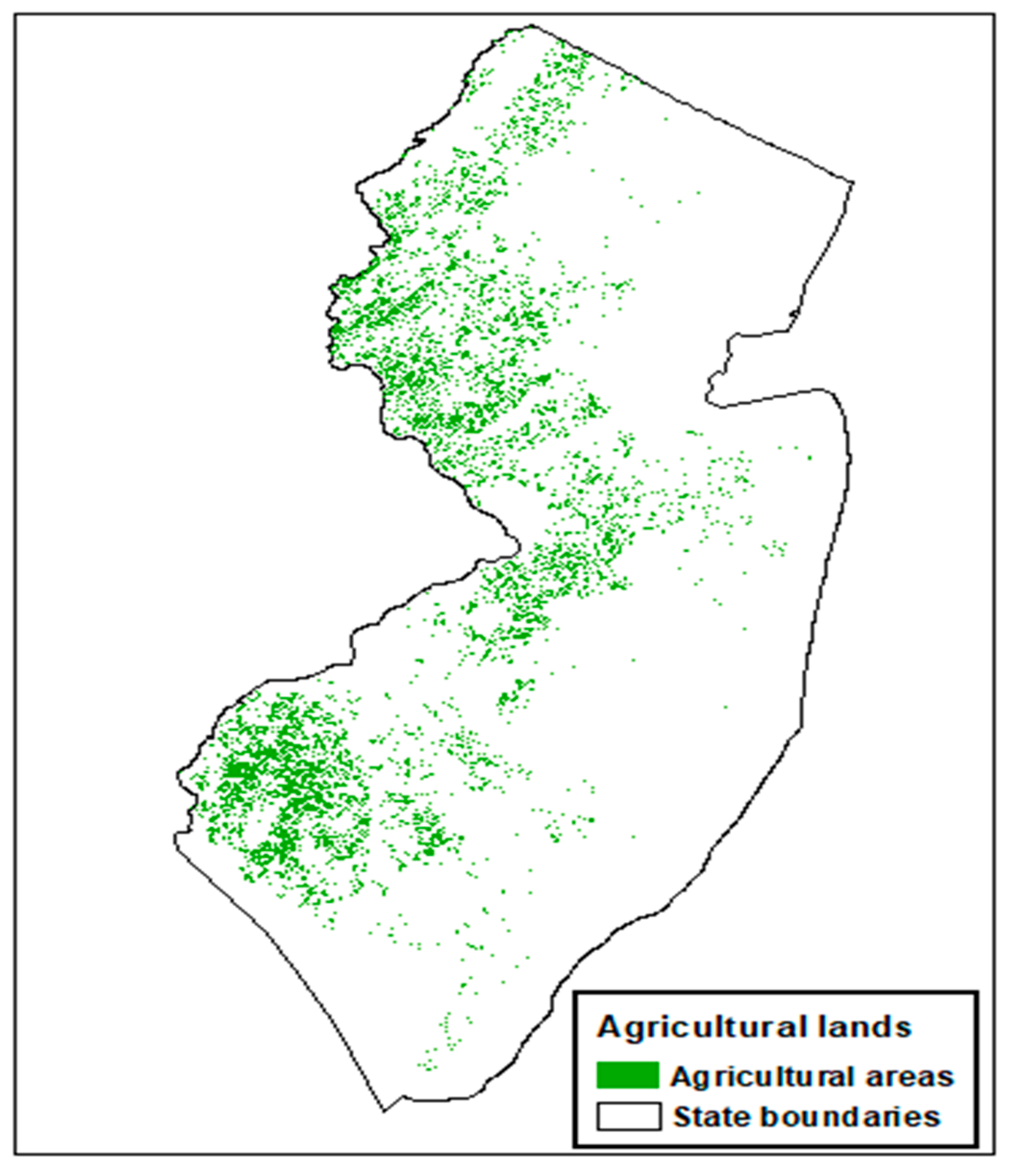
2.1. Study Site and Crop Species

New Jersey covers a land area of 22,610 km2 (Figure 1). With the 2019 population estimate of 8,882,190 [36], New Jersey is the most densely populated state in the United States of America with 458 people per km2 [37,38]. Despite its small size and large population, New Jersey has approximately 9000 remaining farms and is one of the top 10 producers of blueberries, cranberries, peaches, tomatoes, bell peppers, eggplant, cucumbers, apples, spinach, squash, and asparagus in the United States (https://www.nj.gov/agriculture/about/overview.html).
The growth of crops in the state depends not only on bioclimatic factors but also on the spatial distribution of soil texture and structure. For instance, the New Jersey Pine Barrens occupies 1.1 million acres in the southern region of the state is characterized by sandy and acidic soil. Blueberry and cranberry are native to that region and farming of these two species has been fundamental to the Pine Barrens culture and economy for generations. Even though cranberry can grow wild in wet fields, meadows, bogs and along streams in the region it is mass produced in human-made bogs (https://whyy.org/segments/how-farmers-in-new-jerseys-pinelands-grapple-with-the-environmental-toll-of-thanksgiving-cranberries/). Blueberries, on the other hand, grow in the more upland, dry soil [39].
The other crops that we are focusing on grow predominantly in well-drained soils. They include loamy and sandy loamy soils. These types of soils are formed in loamy fluviomarine deposits and are suitable for agricultural use [40]. New Jersey has plenty of loamy and sandy loamy soils that are best for tomato production [41]. New Jersey’s clay loam is ideal for sweet corn [42]. The state is the 6th leading squash producer in the nation [34]. The last crop in our study is squash. It also prefers, well drained, fertile soil, high in organic matter [43]. This type of soil is mostly found in the southern part of the state where 70% of squashes are produced in summer [44].

2.2. Data and Software

We used TerrSet Geospatial Monitoring and Modeling System software [45]. One of the eight toolsets on this software is the Climate Change and Adaptation Modeler (CCAM). Its purpose is to address the issues of a rapidly changing global climate [46]. CCAM has an interface to predict future global climate change up to 2100 under a variety of management scenarios using the coupled MAGICC [16,47] and SCENGEN models [48]. It was developed in conjunction with the fourth assessment of the Intergovernmental Panel on Climate Change (IPCC) [49].
We specified the parameters prior to running MAGICC. We used A1FI-MI and B1TME [46] as the two types of the emission scenarios for our study. A1FI-MI represents the world that is in a situation of high-energy demand, global cooperation and new alternative technologies [46,48]. It is the world of the fossil fuel-intensive combination of coal and oil. We selected this scenario because we believe this situation is relatively similar to the one in which we live today. B1TME represents global cooperation and economic, social, and environmental sustainability with a shift away from fossil fuels and towards enhanced energy conservation—the goal of the Paris Agreement [50,51]. Previous studies have used A1F1 which is a scenario closer to ours [16,31]. The B1 scenario family is slightly similar to A1 and the main difference is the emphasis on clean and sustainable energy production. It is a situation very close to the description we provided for B1TME.
In addition to A1FI-MI and B1TME we applied the following parameters to each of these scenarios. We set the carbon cycle to the mid-range of 1.1 GtC/Year [52,53,54] as also advised by the software builders. We included carbon cycle climate feedbacks. We set thermohaline circulation to variable with the assumption that it will likely slow as the temperature increases. The aerosol forcing was set to the moderate level of −1.3 W/m2 [55,56,57]. The vertical diffusion, a rate of mixing ocean water, was set at 2.3 cm2/s. It is the median value of seven models included in the software [46]. The level of ice melt was based on the central estimates specified in the IPCC Third Annual Report [58]. The sensitivity, Earth’s temperature reaction to doubling of CO2, was set to 3 °C. This value is within the IPCC-recommended values between 0.5 and 5.5 °C [25]. The reference year for climate model output was 1990 and the last year is 2100.
We then run the model for the two scenarios to generate the temperatures in degrees Celsius. Outputs from running SCENGEN generated eight projected global images including four for precipitation and four for temperatures. We averaged 18 models to generate the data we used in this study. The two models, that had a very low statistical correlation, were removed from the suggested 20 models after a preliminary run (Table 1) [46].
SCENGEN image outputs include four maps projected global spatial distribution of monthly, seasonal as well as annual temperatures and precipitation patterns by the end of the century. The first one represents the average of absolute changes in temperatures or precipitation for the 30-year interval centered on 2064, averaged over the 18 selected models (ABSDEL). A second image characterizes the new mean state using a model-mean baseline when including aerosols (ABS-MOD). A third illustrates the new mean state using an observed baseline when including aerosols (ANS-OBS). The fourth image is the scaled change field when only aerosols are included (AEROSOL). Our study focused on ANS-OBS in part because it uses observed data as the baseline and the difference from ABS-MOD was relatively small in most cases it was less than 1 °C.
The ground resolution of maps resulting from running SCENGEN is 2.5 longitudes by 2.5 degrees latitudes. That is, the pixel ground resolution of this global model is about 85 km longitude by 110 km latitude when calculated within the state of New Jersey. The state is elongated and relatively small covering about 22,610 km2, with the south-north distance averaging 240 km and east–west distance of 100 km. The state is actually spread only over smaller parts of each of the four pixels resulting from SCENGEN’s images. A detail spatial analysis of climatic variables and crops distribution is relatively difficult at this coarse resolution.
We decided to run the Downscale Scenario model within the CCAM. This model produces a higher resolution image from a low-resolution image generated through SCENGEN. Previous studies have found no clear evidence of a difference when using downscaling techniques [26,27,59]. The datasets for the entire United States including average monthly and annual climatic conditions over 30 years (1981–2010) were downloaded from PRISM Climate Group [60]. These Climate Normals had pixels representing an 800-m ground resolution, which is a finer resolution compared to SCENGEN’s image resolution. Since our study area is New Jersey, we extracted datasets related only to the state using Geographic Information Systems (GIS) and used these datasets as a baseline. The fine resolution baseline of each image from PRISM Climate group represents an average of climatic variables from 1981–2010 while SCENGEN uses reference datasets over a period from 1980 to 1999. We are assuming in our study that these conditions are relatively similar between these reference periods.
We also run the Crop Climatic Suitability Modeling tool within the CCAM for the following crops: blueberry, cranberry, squash, sweet corn and tomato. The purpose is to project the global suitability distribution of the 5 selected crops in New Jersey based on future monthly temperature and precipitation data, and the length of a crop’s growing season within the state [20,45]. We retrieved required crop bioclimatic parameters from a database developed by the FAO located within CCAM model. We run the model to create suitability maps of our selected crops within New Jersey.
We run Habitat suitability mapping and species modeling. This module relies on a variety of data to detect environmental variability. It derives bioclimatic variables from extreme and average temperature and precipitation data to facilitate a better spatial and temporal environmental interpretation. These derived data represent annual trends, seasonality, and extreme or limiting factors.
We also used additional data for the purpose of having a more general view of spatial patterns for a graphical analysis. The georeferenced dataset of 2015 Land Use/Land Cover of New Jersey was downloaded from [61]. Using GIS, we only selected agricultural lands managed as they related to this study. Unfortunately, this category included cropland and pastureland. It did not provide a detail spatial distribution of specific crops, such as sweet corn, cranberries, potatoes and many more that are farmed in New Jersey.
There is considerable confidence that climate models provide credible quantitative estimates of future climate change, particularly at continental scales and above. This confidence comes from the foundation of the models in accepted physical principles and from their ability to reproduce observed features of current climate and past climate changes. Confidence in model estimates is higher for some climate variables (e.g., temperature) than for others (e.g., precipitation) [49]. Over several decades of development, models have consistently provided a robust and unambiguous picture of significant climate warming in response to increasing greenhouse gases [49].

3. Results

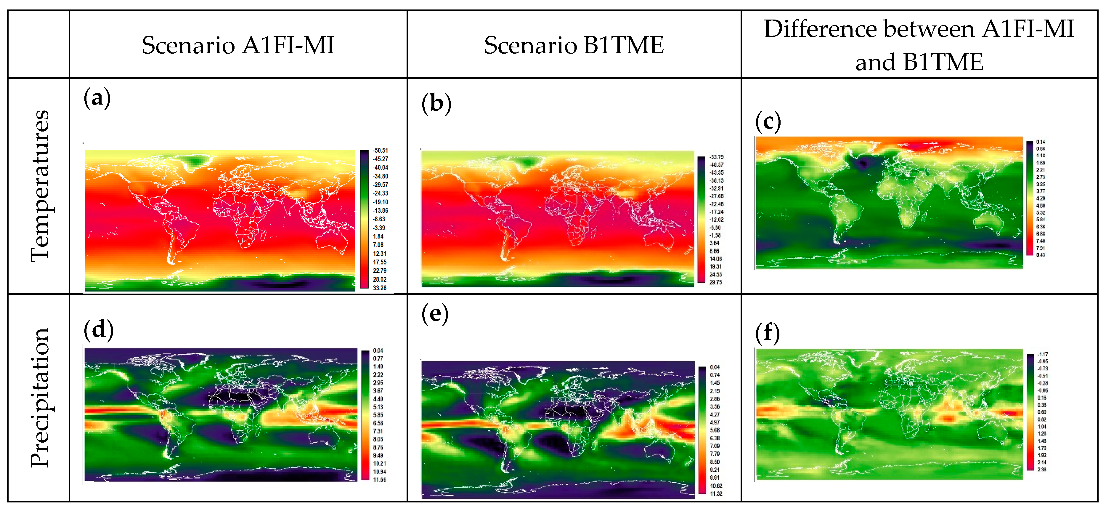
3.1. Global Pattern of Climate Change

There are similarities in the overall spatial distribution of bioclimatic variables between the projection from our two scenarios and the results from IPCC AR4 report [49]. Images from A1FI-MI and B1TME scenarios (Figure 2a,b,d,e), display latitudinal variabilities as one moves away from the equator. According to Table 2 Scenario A1FI-MI, the lowest temperature is −47.34 °C and is located in South Pole regions and in the B1TME scenario it is −50.42 °C. The global temperatures from our models is on average 3 °C cooler in scenario B1TME than in scenario A1FI-MI. The largest difference between our two scenarios is found in the North Pole region while the lowest is in the northern Atlantic Ocean and the southern ocean regions. On land, it varies mostly between 2.7 and 4.3 °C (Figure 2c). With reference to global distribution of annual precipitation, there are no significant differences between the two scenarios (Figure 2d–f, and Table 3). The part of the world likely to have more precipitation is concentrated along the Equatorial region. It decreases as one moves away from this region.

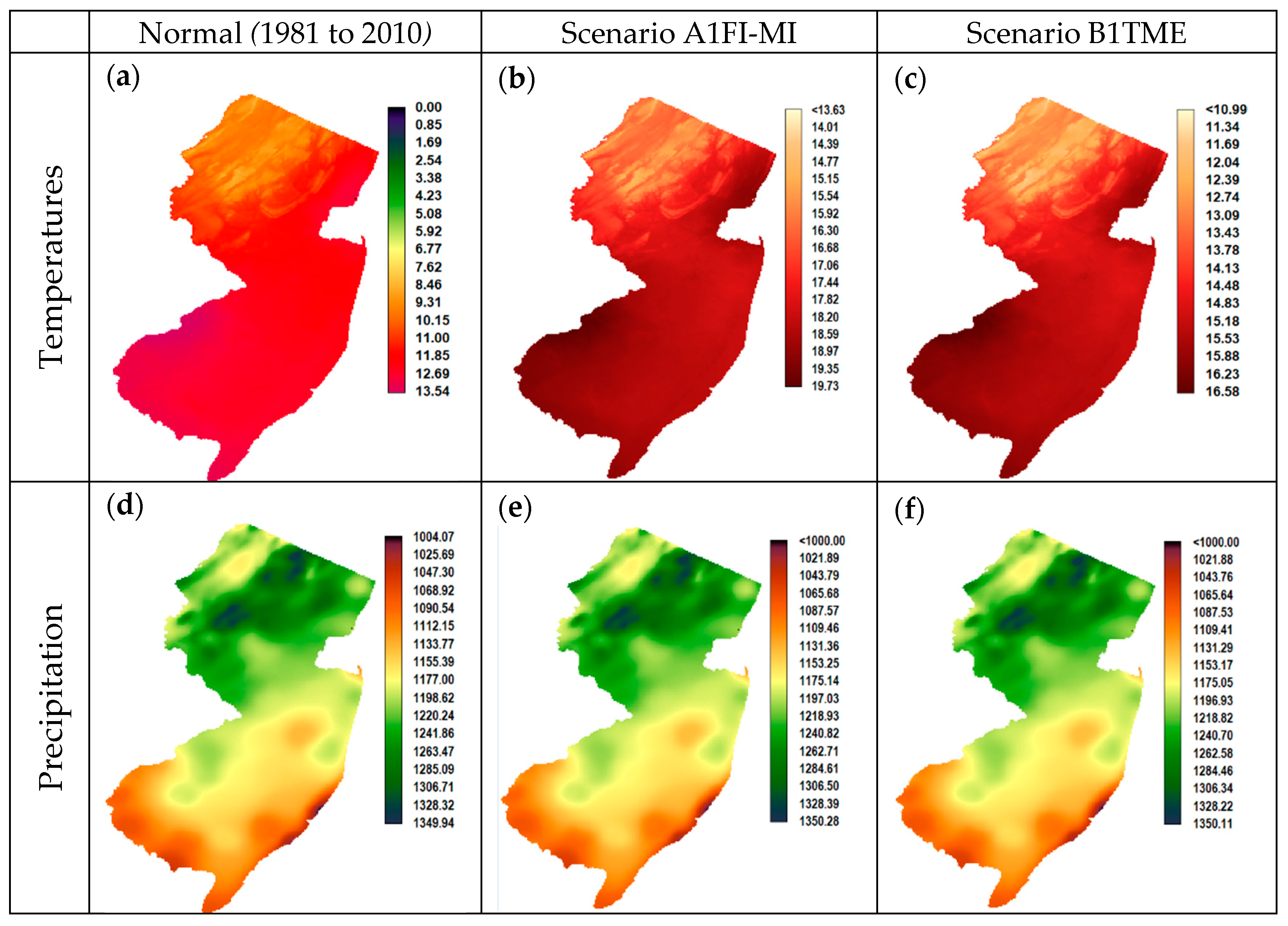
3.2. Downscale Results of the State of New Jersey

3.2.1. Annual Overview of the Models

The data map from PRISM [60] (Figure 3a) shows a pattern similar to the one presented by the Office of the New Jersey State Climatologist [62]. Warmer temperatures are found mostly in the southern part of the state and becoming colder as one moves north especially in northwest in mountainous areas. The hottest climate normal annual temperature of 13.54 °C is in the southwestern part of the state while the coldest, 9 °C, is found in mountainous region in the northeast. Table 4 shows that the average temperature is consistent with the 30-year normal from the office of the New Jersey State Climatologist [63]. The normal for the annual precipitation shows a south-north increase (Figure 3d). In the south, it is around 1000 mm while in the mountainous region of the northwest it is on average more than 1200 mm a year. We averaged the annual precipitation for the entire state and found that it is 1187.16 mm (Table 5).
Results from A1FI-MI and B1TME scenarios (Figure 3b,c) display a similar spatial pattern as in Figure 3a. That is, the southern New Jersey is hotter and becoming colder toward the north of the state. Despite the similarity in the spatial pattern, temperatures are hotter under the two projected scenarios than those of the 30-year normal. The average mean annual temperatures for the entire state of New Jersey using scenarios A1FI-MI and B1TME are 17.94 and 14.79 °C, respectively (Table 4). Under A1FI-MI, the mean annual temperatures increase by more than 6 °C, while under B1TME it increases by about 3 °C when using the 30-year normal as the baseline. The increase is about the same whether we analyze the minimum or the maximum temperatures (Table 4). When we provided global distribution of annual precipitation in the previous section, we found that there was no significant differences between the two scenarios. We found the same results as we look at only the state of New Jersey (Table 5).
Throughout the last century the annual temperatures increased by about 1.65 °C (3°F) under a high Greenhouse gases (GHG) emission scenario [64]. However, if we continue doing business as usual (A1FI-MI scenario) our study projects that the annual temperatures increase will be 6.14 °C. Some studies have projected that by the end of this century the annual precipitation will increase [8,64], our model found that there will not be a significant difference compared to the 30-year (1981–2010) normal.

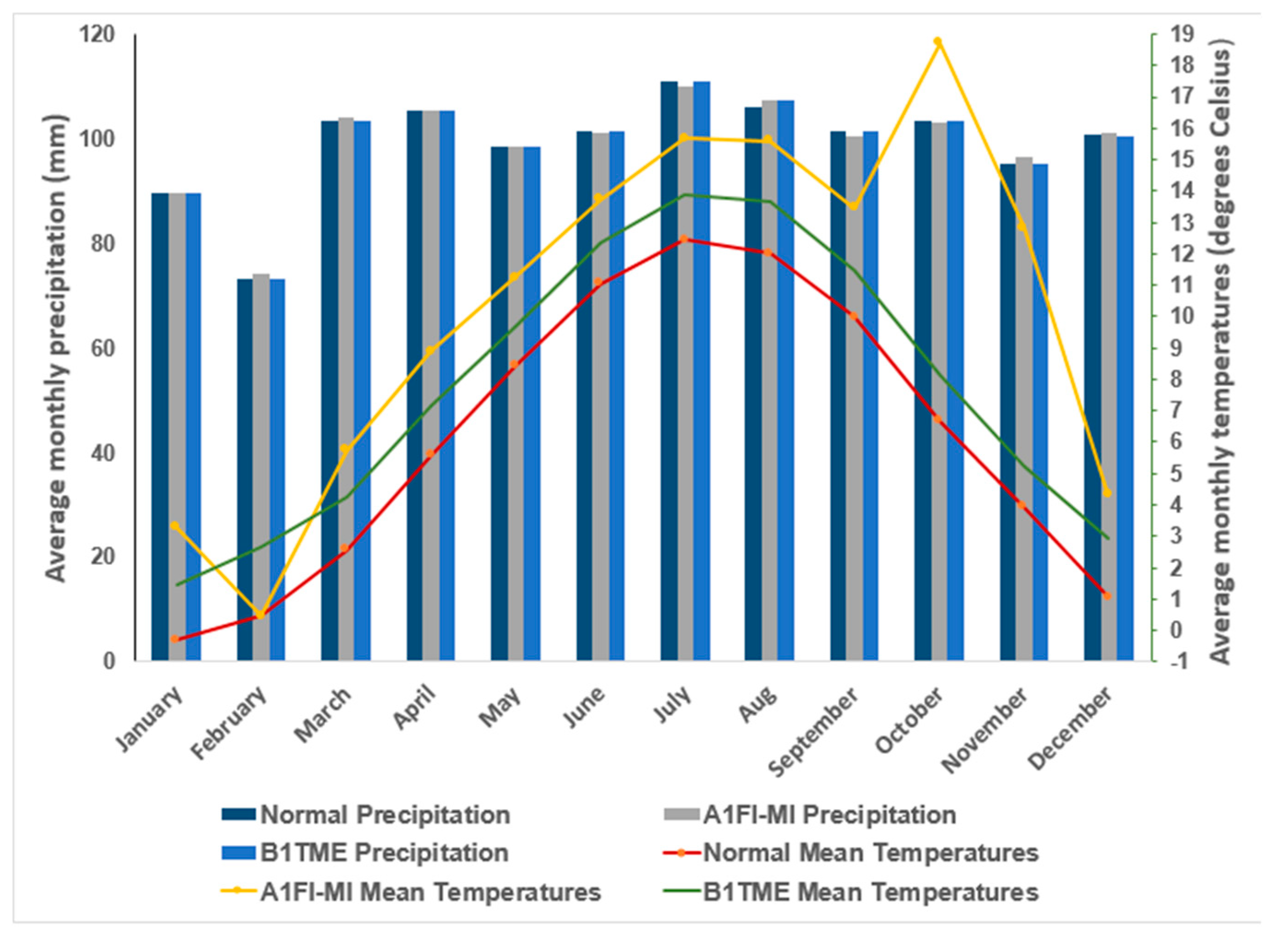
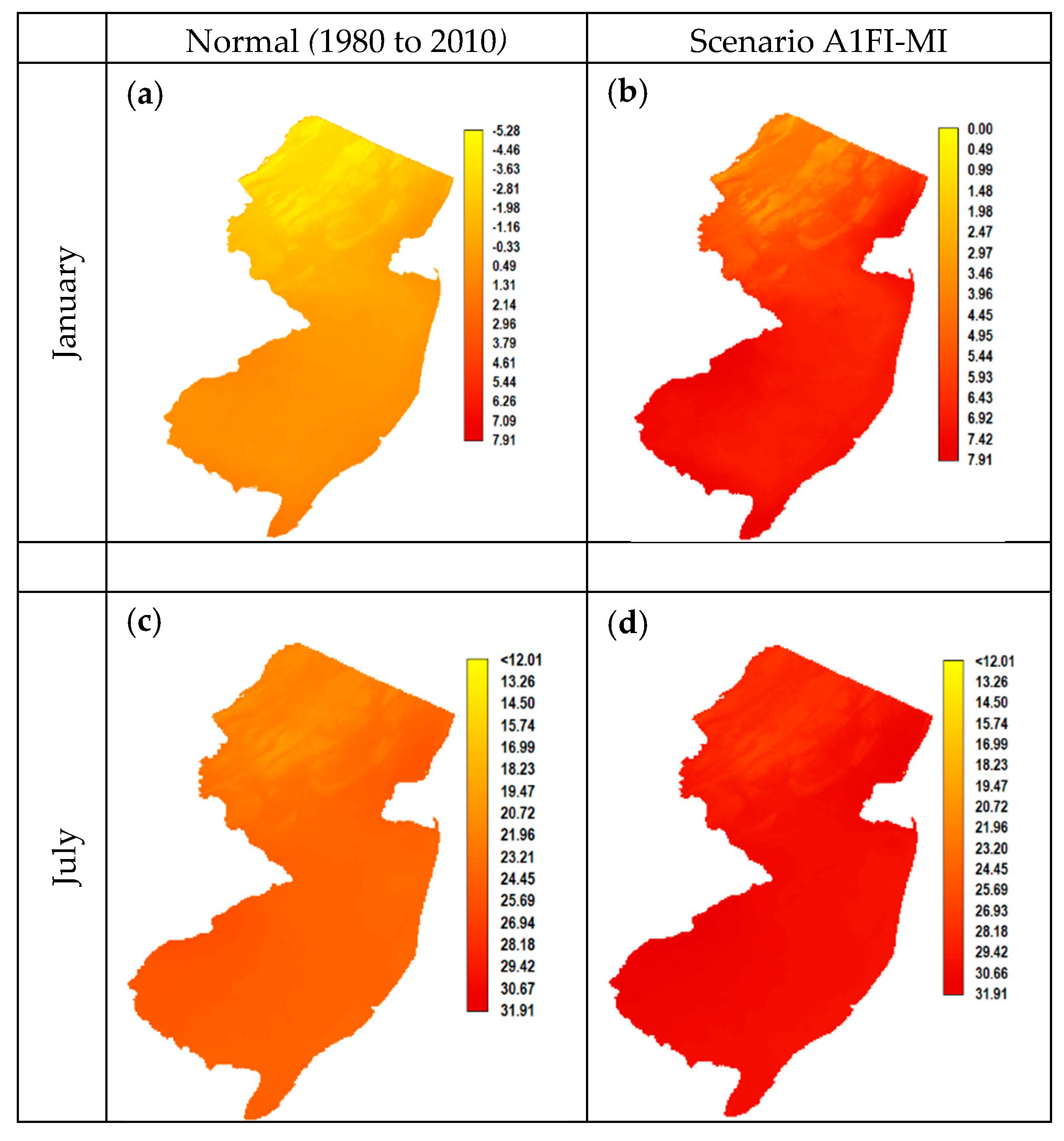
3.2.2. Monthly Analysis

We limited the monthly results to the comparison between data from PRISM and A1FI-MI. We believe that results from these two types of data will highlight the impacts climate change will have on our environment including farming. A1FI-MI is considered as an extreme case scenario and B1TME as a median scenario and very close to the 1981–2010 normal based on the pattern of temperature variation as displayed in Figure 4. By highlighting A1FI-MI scenario, we believe that these results will serve not only as a wake-up call, but also will be useful to decision makers to take appropriate measures to mitigate the impacts likely to prevail by the end of the century if we continue doing business as usual (A1FI-MI scenario).
Our state monthly results show that there is no significant differences in the average precipitation between the 30-year normal (1981–2010) and the projected average precipitation under A1FI-MI scenario (Figure 4). There are, however, variabilities between months. Even though it rains every month in New Jersey throughout the year, in both cases, February has the lowest and July the highest average amount of precipitation. These findings are consistent with the amount of annual precipitation presented in the above sub-section (Table 5) if all monthly precipitation measurements are added together.
As opposed to precipitation, the pattern of monthly average temperatures is variable (Figure 4). The 30-year normal average monthly temperatures follow the seasonal pattern known in New Jersey [63]. Figure 4 shows that winter months are cold, and the coldest month is January with an average monthly temperature of −0.32 °C. Summer is hot and the hottest month is July with an average monthly temperature of 23.82 °C. Under A1FI-MI scenario the temperature is generally hotter than the 30-year normal. The coldest temperature is February with an average of 0.45 °C and the hottest temperature of 19.24 °C in October. We believe these are inexplicable anomalies if we look at the overall pattern of A1FI-MI scenario curve. Therefore, January will be considered the coldest and July the warmer under this scenario. This increase in the coldest and hottest average monthly temperatures will have major consequences on both natural and managed ecosystems including the timing of planting, sprouting, and growing of crops [31].
The spatial distribution of the average monthly temperatures is provided in Figure 5. We selected only January (Figure 5a,b) and July (Figure 5c,d) for illustration. In both cases, the distribution follows the pattern highlighted in Figure 3. That is, the southern part is warmer than the northern part of the state. It also shows that the topography, proximity to water body and urbanization may play some roles in the spatial distribution of these changes. For instance, the northwestern part is mountainous while the southern part is in the lowlands. The northeastern and southwestern regions are densely populated and more urbanized. Most of the southern and eastern are surrounded by ocean.

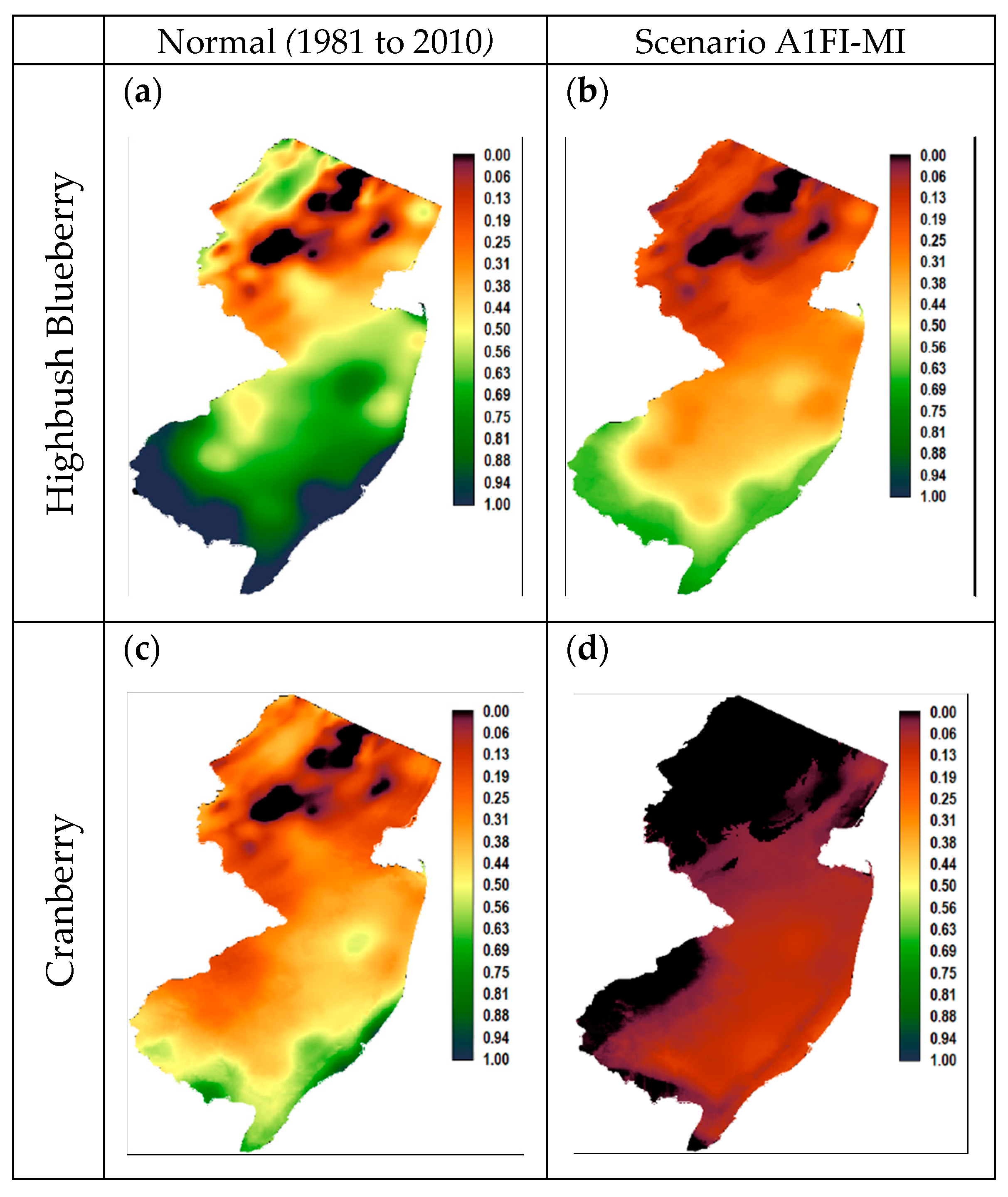
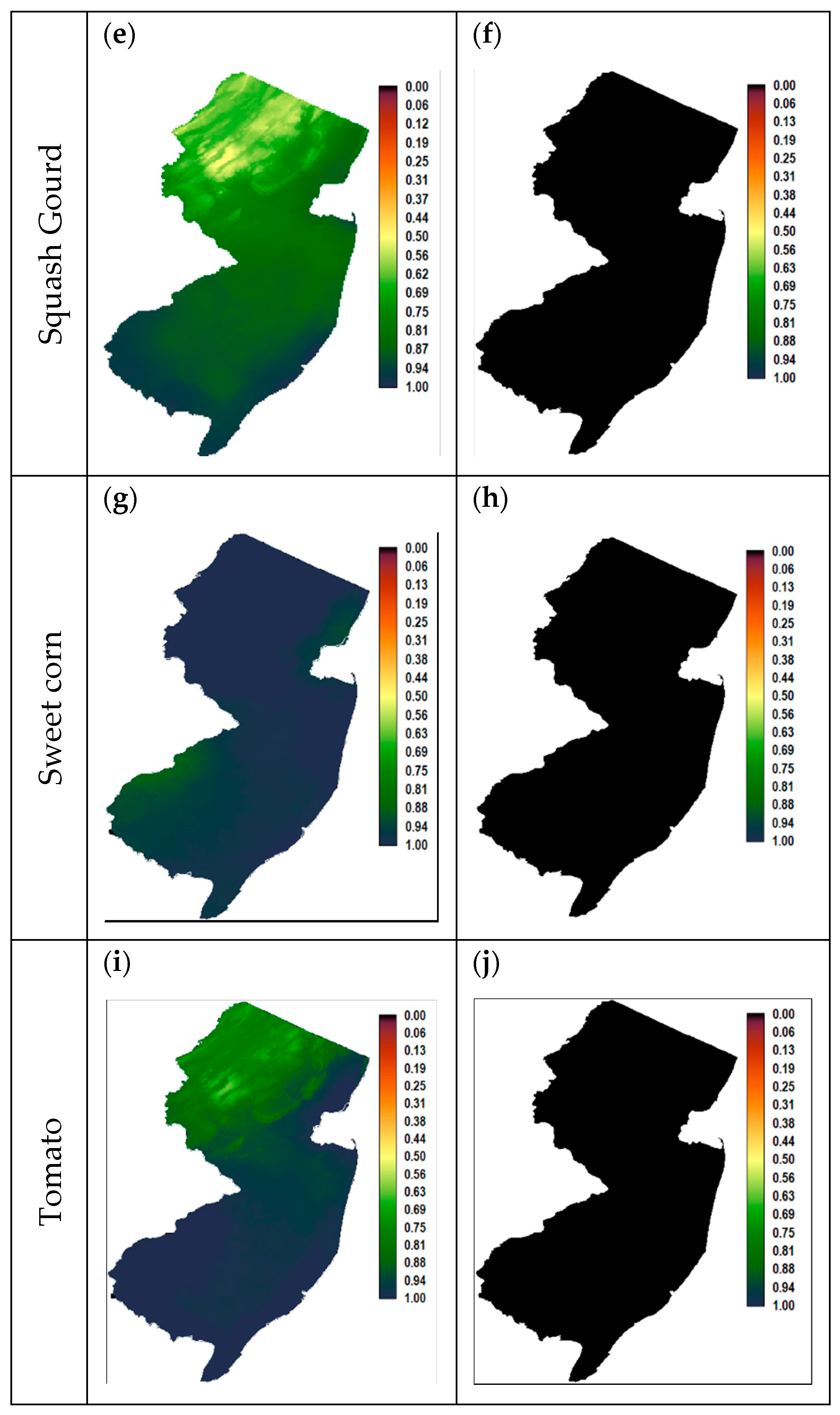
3.2.3. Impacts on Suitability to Crops

We used the 1981–2010 distribution map results as the baseline, as seen in Figure 6a,c,e,g,i. Table 6 provides the interpretation scheme presented on the legends of every map [65]. The baseline maps show the potential extent to grow squash, sweet corn, and tomato varies from highly to very suitable throughout the entire state (Figure 6e,g,i). For blueberry and cranberry (Figure 6a,b) it is highly and very suitable in south and becomes medium and marginally suitable in the northern part of the state. Compared to A1FI-MI scenario, results (Figure 6d,f,h,j) show that the suitability for cranberry, squash, sweet corn, and tomato becomes very marginal throughout the state. For the blueberry (Figure 6b) the suitability moves to very suitable in the south and very marginal in the north.
The maps presented on Figure 6 display potential areas suitable for these crops. These areas may include forested and grass lands, urbanized areas, the road network, water bodies where these crops are not grown. The true extent of suitable crop lands is very restricted if we exclude these areas. Figure 7 shows the actual agricultural lands and was obtained from 2015 Land Use/Land Cover using Geographic Information Systems (GIS).

4. Discussion

Although the map was developed using New Jersey Department of Environmental Protection Geographic Information System digital data, the agricultural lands have not been verified by NJDEP and are not state-authorized or endorsed [61]. The ground resolution of the digital imagery from which the vector map was created is about 1 by 1 m and is characterized as fine resolution and the accuracy is very high. It is remarkably clear that in this highly industrial and densely populated state, we are in danger of losing what remains to future development. As such, Figure 7 is a warning to all of us—and especially to the decision makers—that in order to sustain today’s environment we need to change our behavior and take appropriate actions.
More importantly, these models do not take into account indirect effects of climate change on crops. For example, a warmer climate will likely allow certain weeds [66], insect pests, and crop diseases, to thrive in New Jersey. The New Jersey Agriculture Experiment Station warns that milder and shorter winters may not kill off certain insect pests or crop diseases, increasing the chances for greater issues [67]. For example, pest species, including the tomato pinworm, commonly found in the southwestern states, was found in New Jersey starting in 2012. In addition, fires have been increasing in severity globally by virtue of climate change. The Pine Barrens occupy of southern New Jersey has evolved with low-intensity fires as part of the natural disturbance regime and it is also the primary location of cranberry and blueberry farming in the state. Increasingly, however, this fire-adapted ecosystem has accumulated more fuel, as trees have been lost to pests that thrive in warmer temperatures, and therefore fires that do occur are in danger of becoming more intense and damaging to the communities and farmland in the region [68].
New farming techniques have already started to be implemented in New Jersey to sustain the impact of climate change. For instance, aeroponics is a technique that does not require soil and sun for farming. AeroFarms’ system sprays plants with a nutrient-rich mist. Seeds are sown, germinated, and grown on reusable sheets of fabric [69]. Hydroponic agriculture is another technique used in New Jersey. The roots of the crops are “dangling down into water, and so they’re not only immersed in that water, and are able to take up that water when they need it, but the nutrients that those plants need is also in the water itself” [70]. This technique makes it possible to grow crops all year around. In addition to these alternative forms of agriculture, the farming industry is increasing relying on genetically modified organism (GMO) for crops such as soy and corn [71,72]. The GMO technique involves the transferring of one or more genes that tolerate herbicide or resist pests (such as from a bacteria) into the plant. It is clear that with more people to feed, less land to farm, and a changing climate, there will be an ever-increasing demand for innovative farming techniques such as these.

5. Conclusions

Our results are corroborated by other studies. For instance, we found that under A1FI-MI the mean annual temperatures will increase by more than 6 °C, while under B1TME it will increase by about 3 °C in New Jersey. Results from the Intergovernmental Panel on Climate Change (IPCC) found an increase of global mean surface temperature by the end of the 21st century to vary between 2.6 and 4.8 °C under the RCP8.5 scenario [73]. Meehl et al. [21] also found that it will range from 2.4 to 6.4 °C under A1FI scenario. With reference to precipitation, our model found that there will not be a significant difference compared to the 30-year (1981–2010) normal. The IPCC report found that some areas in mid-latitude regions will experience a decrease while others an increase [73]. Meehl et al. [21] projected an increase in precipitation extremes by 2100.
The United States Environmental Protection Agency (US EPA) reports that over the last century, the mean annual precipitation in New Jersey has increased 5–10% and is projected to continue to rise. The EPA projected that throughout the Northeast, precipitation from extremely heavy storms has increased 70% over the past 60 years and will likely continue to increase during winter and spring, but not change significantly during summer and fall. Simultaneously, however, rising temperatures will melt snow earlier in spring causing river flooding, and dry the soil during summer and fall, bringing drought during the growing season [74]. Our findings from this research bring these regional predictions down to the state level and show that even though the mean annual precipitation will remain relatively the same, it will become more extreme (Table 3). It is important to also note that while steady annual precipitation is important for plants, the fact that our model predicts changes distribution throughout the year is troublesome. The temperature increase will likely lead to more rain and flooding in February and March (Figure 4) in New Jersey. Hotter temperatures are likely to lead to more evaporation and drier soils.
We have demonstrated that climate change will affect the state of New Jersey. Using CCAM we have shown how climate change will change the spatial extent of crops such as blueberry, cranberry, squash, sweet corn and tomato. The impacts may not be limited to these crops. The negative effects on crops has the potential to undermine the economy of the state and the wellbeing of its citizens. Our study also demonstrates that downscaling is an appropriate method to project future climate and to evaluate crop suitability resulting from climate change. This study will help decision makers and spatial planers to come up with strategies to mitigate the impacts for a more sustainable future [75]. This study also may help promote climate-resilient staples and alternative crops [76].
Although the study focused on New Jersey, the effects of climate change on the environment including agriculture do not have boundaries. Studies have found that climate change will have an impact on agriculture and food security [9,77,78]. This emphasizes the need for global cooperation in designing and adapting plans to cope with climate change. The Paris Agreement marks a step in the right direction [51,79], presenting opportunities for the agricultural industry worldwide to mitigate and adapt to climate change. Similarly, the Intergovernmental Panel on Climate Change’s report on Food Security points out that climate change is already affecting food availability through increasing temperatures, changing precipitation patterns and greater frequency of extreme events [73]. The IPCC notes that there needs to be a global effort throughout the food system through policies, markets, institutions and governance to mitigate and adapt to a rapidly changing climate on the global scale. Through the research presented in this paper, we have demonstrated the need to recognize what climatic changes at the state level can have on specific crops. We have focused on five crops that play important roles in the diet, economy and culture of New Jersey, recognizing that these crops are just samples of the countless other species that are already being affected by climate change.

Author Contributions

Conceptualization, K.I.N.; methodology, K.I.N. and D.S.; software, K.I.N.; formal analysis, K.I.N. and D.S.; writing—original draft preparation, K.I.N.; writing—review and editing, D.S. All authors have read and agreed to the published version of the manuscript.

Funding

This research received no external funding.

Acknowledgments

We would like to thank the School of Environmental and Sustainability Sciences for the software used in this study.

Conflicts of Interest

The authors declare no conflict of interest.

References

  1. Climate Change and Human Health: Risks and Responses; McMichael, A.J. (Ed.) World Health Organization: Geneva, Switzerland, 2003. [Google Scholar]
  2. Arnell, N. Climate change and global water resources. Glob. Environ. Chang. 1999, 9, S31–S49. [Google Scholar] [CrossRef]
  3. Hagemann, S.; Chen, C.; Clark, D.B.; Folwell, S.; Gosling, S.N.; Haddeland, I.; Hanasaki, N.; Heinke, J.; Ludwig, F.; Voss, F.; et al. Climate change impact on available water resources obtained using multiple global climate and hydrology models. Earth Syst. Dyn. 2013, 4, 129–144. [Google Scholar] [CrossRef] [Green Version]
  4. Jacob, D.J.; Winner, D.A. Effect of climate change on air quality. Atmos. Environ. 2009, 43, 51–63. [Google Scholar] [CrossRef] [Green Version]
  5. Fischer, G.; Shah, M.; Tubiello, F.N.; Van Velhuizen, H. Socio-economic and climate change impacts on agriculture: An Integrated assessment, 1990–2080. Philos. Trans. R. Soc. B 2005, 360, 2067–2083. [Google Scholar] [CrossRef]
  6. Gbetibouo, G.A.; Hassan, R.M. Measuring the economic impact of climate change on major South African field crops: A Ricardian approach. Glob. Planet. Chang. 2005, 47, 143–152. [Google Scholar] [CrossRef]
  7. Levy, P.E.; Cannell, M.G.R.; Friend, A.D. Modelling the impact of future changes in climate, CO2 concentration and land use on natural ecosystems and the terrestrial carbon sink. Glob. Environ. Chang. 2004, 14, 21–30. [Google Scholar] [CrossRef]
  8. Christensen, J.H.; Hewitson, B.; Busuioc, A.; Chen, A.; Gao, X.; Held, I.; Jones, R.; Kolli, R.K.; Kwon, W.-T.; Mearns, L.; et al. Regional climate projections. In Climate Change 2007: The Physical Science Basis. Contribution of Working Group I to the Fourth Assessment Report of the Intergovernmental Panel on Climate Change; Solomon, S., Qin, D., Manning, M., Chen, Z., Marquis, M., Averyt, K.B., Tignor, M., Miller, H.L., Eds.; Cambridge University Press: Cambridge, UK; New York, NY, USA, 2007; p. 94. [Google Scholar]
  9. Food and Agriculture Organization (FAO). Climate change, agriculture and food security. In The State of Food and Agriculture; FAO: Rome, Italy, 2016. [Google Scholar]
  10. Hatfield, J.L.; Boote, K.J.; Kimball, B.A.; Ziska, L.H.; Izaurralde, R.C.; Ort, D.; Thomson, A.M.; Wolfe, D. Climate impacts on agriculture: Implications for crop production. Agron. J. 2011, 103, 351. [Google Scholar] [CrossRef] [Green Version]
  11. Niles, M.T.; Lubell, M.; Brown, M. How limiting factors drive agricultural adaptation to climate change. Agric. Ecosyst. Environ. 2015, 200, 178–185. [Google Scholar] [CrossRef] [Green Version]
  12. del Río, S.; Cano-Ortiz, A.; Herrero, L.; Penas, A. Recent Trends in mean maximum and minimum air temperatures over Spain (1961–2006). Theor. Appl. Climatol. 2012, 109, 605–626. [Google Scholar] [CrossRef]
  13. Del Río, S.; Iqbal, M.A.; Cano-Ortiz, A.; Herrero, L.; Hassan, A.; Peñas, A. Recent mean temperature trends in Pakistan and links with teleconnection patterns. Int. J. Climatol. 2013, 33, 277–290. [Google Scholar] [CrossRef]
  14. Ren, G.; Ding, Y.; Tang, G. An overview of mainland China temperature change research. J. Meteorol. Res. 2017, 31, 3–16. [Google Scholar] [CrossRef]
  15. Cano, E.; Cano-Ortiz, A.; Musarella, C.M.; Fuentes, J.C.P.; Ighbareyeh, J.M.H.; Gea, F.L.; Del Río, S. Mitigating climate change through bioclimatic applications and cultivation techniques in agriculture (Andalusia, Spain). In Sustainable Agriculture, Forest and Environmental Management; Jhariya, M.K., Banerjee, A., Meena, R.S., Yadav, D.K., Eds.; Springer: Singapore, 2019; pp. 31–69. [Google Scholar] [CrossRef]
  16. Special Report on Emissions Scenarios: A Special Report of Working Group III of the Intergovernmental Panel on Climate Change; Nakićenović, N.; Intergovernmental Panel on Climate Change (Eds.) Cambridge University Press: Cambridge, UK; New York, NY, USA, 2000. [Google Scholar]
  17. Buis, A. Study Confirms Climate Models are Getting Future Warming Projections Right. Available online: https://climate.nasa.gov/news/2943/study-confirms-climate-models-are-getting-future-warming-projections-right (accessed on 1 August 2020).
  18. Parry, M. Global impacts of climate change under the SRES scenarios. Glob. Environ. Chang. 2004, 14, 1. [Google Scholar] [CrossRef]
  19. Lenssen, N.J.L.; Schmidt, G.A.; Hansen, J.E.; Menne, M.J.; Persin, A.; Ruedy, R.; Zyss, D. Improvements in the GISTEMP uncertainty model. J. Geophys. Res. Atmos. 2019, 124, 6307–6326. [Google Scholar] [CrossRef]
  20. WorldClim. Global Climate and Weather Data—WorldClim 1 Documentation. Available online: https://www.worldclim.org/data/index.html (accessed on 17 July 2020).
  21. Meehl, G.A.; Stocker, T.F.; Collins, W.D.; Friedlingstein, P.; Gaye, A.T.; Gregory, J.M.; Kitoh, A.; Knutti, R.; Murphy, J.M.; Noda, A.; et al. Global climate projections. In Climate Change 2007: The Physical Science Basis. Contribution of Working Group I to the Fourth Assessment Report of the Intergovernmental Panel on Climate Change; Cambridge University Press: Cambridge, UK, 2007; pp. 747–846. [Google Scholar]
  22. Iglesias, A.; Garrote, L.; Quiroga, S.; Moneo, M. A regional comparison of the effects of climate change on agricultural crops in Europe. Clim. Chang. 2012, 112, 29–46. [Google Scholar] [CrossRef] [Green Version]
  23. Wang, Y.; Leung, L.R.; McGregor, J.L.; Lee, D.-K.; Wang, W.-C.; Ding, Y.; Kimura, F. Regional climate modeling: Progress, challenges, and prospects. J. Meteorol. Soc. Jpn. 2004, 82, 1599–1628. [Google Scholar] [CrossRef] [Green Version]
  24. Wolfe, D.W.; Ziska, L.; Petzoldt, C.; Seaman, A.; Chase, L.; Hayhoe, K. Projected change in climate thresholds in the Northeastern U.S.: Implications for crops, pests, livestock, and farmers. Mitig. Adapt. Strateg. Glob. Chang. 2008, 13, 555–575. [Google Scholar] [CrossRef] [Green Version]
  25. Fordham, D.A.; Wigley, T.M.L.; Watts, M.J.; Brook, B.W. Strengthening forecasts of climate change impacts with multi-model ensemble averaged projections using MAGICC/SCENGEN 5.3. Ecography 2012, 35, 4–8. [Google Scholar] [CrossRef]
  26. Fujimori, S.; Abe, M.; Kinoshita, T.; Hasegawa, T.; Kawase, H.; Kushida, K.; Masui, T.; Oka, K.; Shiogama, H.; Takahashi, K.; et al. Downscaling global emissions and its implications derived from climate model experiments. PLoS ONE 2017, 12, e0169733. [Google Scholar] [CrossRef] [Green Version]
  27. Latombe, G.; Burke, A.; Vrac, M.; Levavasseur, G.; Dumas, C.; Kageyama, M.; Ramstein, G. Comparison of spatial downscaling methods of general circulation model results to study climate variability during the last glacial maximum. Geosci. Model Dev. 2018, 11, 2563–2579. [Google Scholar] [CrossRef] [Green Version]
  28. Dupigny-Giroux, L.-A.; Mecray, E.; Lemcke-Stampone, M.; Hodgkins, G.A.; Lentz, E.E.; Mills, K.E.; Lane, E.D.; Miller, R.; Hollinger, D.; Solecki, W.D.; et al. Chapter 18: Northeast. Impacts, Risks, and Adaptation in the United States: The Fourth National Climate Assessment, Volume II; U.S. Global Change Research Program: Washington, DC, USA, 2018.
  29. Frumhoff, P.C.; McCarthy, J.J.; Melillo, J.M.; Moser, S.C.; Wuebbles, D.J. Confronting Climate Change in the U.S. Northeast: Science, Impacts, and Solutions. Synthesis Report of the Northeast Climate Impacts Assessment (NECIA); Union of Concerned Scientists (UCS): Cambridge, MA, USA, 2007. [Google Scholar]
  30. Hayhoe, K.; Wake, C.; Anderson, B.; Liang, X.-Z.; Maurer, E.; Zhu, J.; Bradbury, J.; DeGaetano, A.; Stoner, A.M.; Wuebbles, D. Regional climate change projections for the Northeast USA. Mitig. Adapt. Strateg. Glob. Chang. 2008, 13, 425–436. [Google Scholar] [CrossRef]
  31. Hayhoe, K.; Wake, C.P.; Huntington, T.G.; Luo, L.; Schwartz, M.D.; Sheffield, J.; Wood, E.; Anderson, B.; Bradbury, J.; DeGaetano, A.; et al. Past and future changes in climate and hydrological indicators in the US Northeast. Clim. Dyn. 2007, 28, 381–407. [Google Scholar] [CrossRef]
  32. Iverson, L.; Prasad, A.; Matthews, S. Modeling Potential climate change impacts on the trees of the Northeastern United States. Mitig. Adapt. Strateg. Glob. Chang. 2008, 13, 487–516. [Google Scholar] [CrossRef]
  33. Lynch, C.; Seth, A.; Thibeault, J. Recent and projected annual cycles of temperature and precipitation in the Northeast United States from CMIP5. J. Clim. 2016, 29, 347–365. [Google Scholar] [CrossRef]
  34. Goldman, J. New Jersey’s 10 Most Valuable Crops May Surprise You. Available online: https://www.nj.com/business/2016/06/new_jerseys_10_most_valuable_crops_may_surprise_you.html (accessed on 13 August 2020).
  35. United States Department of Agriculture. USDA—National Agricultural Statistics Service—New Jersey—Annual Statistical Bulletins. Available online: https://www.nass.usda.gov/Statistics_by_State/New_Jersey/Publications/Annual_Statistical_Bulletin/ (accessed on 18 July 2020).
  36. U.S. Census Bureau. U.S. Census Bureau QuickFacts: New Jersey. Available online: https://www.census.gov/quickfacts/NJ (accessed on 8 July 2020).
  37. Duffin, E. Population Density in the U.S., by State 2019. Available online: https://www.statista.com/statistics/183588/population-density-in-the-federal-states-of-the-us/ (accessed on 15 August 2020).
  38. U.S. Census Bureau. Population Clock. Available online: https://www.census.gov/popclock/ (accessed on 8 July 2020).
  39. Pinelands Preservation Alliance. Pinelands Agriculture. Pinelands Preservation Alliance. Available online: https://pinelandsalliance.org/learn-about-the-pinelands/pinelands-history-and-culture/pinelands-agriculture/ (accessed on 8 July 2020).
  40. USDA-NRCS Soil Survey Division. Featured Soil: Downer | NRCS New Jersey. Available online: https://www.nrcs.usda.gov/wps/portal/nrcs/detail/nj/soils/?cid=stelprdb1249821 (accessed on 13 August 2020).
  41. New Jersey Tomatoes: What’s All the Hype About? Available online: https://www.new-jersey-leisure-guide.com/tomatoes.html (accessed on 13 August 2020).
  42. Sweet Corn—Jersey Roadside Farm Stands. Available online: https://www.rt23.com/jersey_corn/index.shtml (accessed on 13 August 2020).
  43. Cornell University. Explore Cornell—Home Gardening—Vegetable Growing Guides—Growing Guide. Available online: http://www.gardening.cornell.edu/homegardening/scene6420.html (accessed on 12 September 2020).
  44. Infante-Casella, M. Crop Profile for Summer and Winter Squash in New Jersey. Available online: http://njinpas.rutgers.edu/CropProfiles/squashprofile.pdf (accessed on 13 August 2020).
  45. Clark Labs. TerrSet Geospatial Monitoring and Modeling Software. Available online: https://clarklabs.org/terrset/ (accessed on 3 July 2020).
  46. Eastman, R.; Clark Labs/Clark University. Available online: https://clarklabs.org/wp-content/uploads/2016/10/Terrset-Manual.pdf (accessed on 9 July 2020).
  47. Meinshausen, M.; Raper, S.C.B.; Wigley, T.M.L. Emulating coupled atmosphere-ocean and carbon cycle models with a simpler model, MAGICC6—Part 1: Model description and calibration. Atmos. Chem. Phys. 2011, 11, 1417–1456. [Google Scholar] [CrossRef] [Green Version]
  48. Wigley, T.M.L. MAGICC/SCENGEN 5.3: USER MANUAL (Version 2); NCAR: Boulder, CO, USA, 2008; p. 81. [Google Scholar]
  49. AR4 Climate Change 2007: The Physical Science Basis—IPCC; Solomon, S.; Qin, D.; Manning, M.; Chen, Z.; Marquis, M.; Averyt, K.; Tignor, M.M.B. (Eds.) Cambridge University Press: Cambridge, UK, 2007. [Google Scholar]
  50. UNFCCC. Paris Agreement. FCCC/CP/2015/L.9/Rev1. Available online: https://unfccc.int/resource/docs/2015/cop21/eng/l09r01.pdf (accessed on 13 July 2020).
  51. UNFCCC. Synthesis Report on the Aggregate Effect of the Intended Nationally Determined Contributions: An Update. FCCC/CP/2016/2. Available online: https://unfccc.int/resource/docs/2016/cop22/eng/02.pdf (accessed on 13 July 2020).
  52. Riebeek, H. The Carbon Cycle. Available online: https://earthobservatory.nasa.gov/features/CarbonCycle (accessed on 13 July 2020).
  53. Climate Change 2007: The Physical Science Basis: Contribution of Working Group I to the Fourth Assessment Report of the Intergovernmental Panel on Climate Change; Solomon, S.; Qin, D.; Manning, M.; Chen, Z.; Marquis, M.; Averyt, K.; Tignor, M.M.B.; Miller, H.L. (Eds.) Cambridge University Press: Cambridge, UK, 2007. [Google Scholar]
  54. Folger, P. The Carbon Cycle: Implication for Climate Change and Congress. Available online: https://fas.org/sgp/crs/misc/RL34059.pdf (accessed on 13 July 2020).
  55. Chung, C.E. Aerosol direct radiative forcing: A review. In Atmospheric Aerosols—Regional Characteristics—Chemistry and Physics; Scitus Academics LLC: Wilmington, NC, USA, 2012. [Google Scholar] [CrossRef] [Green Version]
  56. Eastman, R.; Clark Labs. Available online: https://clarklabs.org/ (accessed on 3 July 2020).
  57. Redden, R.; Materne, M.; Maqbool, A.; Freeman, A. Biodiversity challenges with climate change. In Climate Change and Management of Cool Season Grain Legume Crops; Yadav, S.S., Redden, R., Eds.; Springer: Dordrecht, The Netherlands, 2010; pp. 409–432. [Google Scholar]
  58. Cooper, R.N.; Houghton, J.T.; McCarthy, J.J.; Metz, B. Climate change 2001: The scientific basis. Foreign Aff. 2002, 81, 208. [Google Scholar] [CrossRef]
  59. Manzanas, R.; Gutiérrez, J.M.; Fernández, J.; van Meijgaard, E.; Calmanti, S.; Magariño, M.E.; Cofiño, A.S.; Herrera, S. Dynamical and statistical downscaling of seasonal temperature forecasts in Europe: Added value for user applications. Clim. Serv. 2018, 9, 44–56. [Google Scholar] [CrossRef]
  60. PRISM Climate Group. 30-Year Normals. Available online: https://prism.oregonstate.edu/normals/ (accessed on 17 July 2020).
  61. NJ Department of Environmental Protection (NJDEP). Land Use/Land Cover 2015 Update, Edition 20190128 (Land_lu_2015). Available online: https://www.arcgis.com/sharing/rest/content/items/6f76b90deda34cc98aec255e2defdb45/info/metadata/metadata.xml?format=default&output=html (accessed on 3 August 2020).
  62. Office of the New Jersey State Climatologist. Available online: https://climate.rutgers.edu/stateclim/ (accessed on 23 July 2020).
  63. Environmental Information (NCEI); Office of the New Jersey State Climatologist (ONJSC). ONJSC: Historical Monthly Summary Tables. Available online: http://climate.rutgers.edu/stateclim_v1/nclimdiv/index.php?stn=NJ00&elem=avgt (accessed on 23 July 2020).
  64. Runkle, J.; Kunkel, K.E.; Champion, S.; Frankson, R.; Stewart, B.C.; Sweet, W. New Jersey State Climate Summary. NOAA Technical Report NESDIS 149-NJ. 4p. Available online: https://statesummaries.ncics.org/downloads/NJ-print-2016.pdf (accessed on 29 July 2020).
  65. Abdallah, C.; Jaafar, H. Data set on current and future crop suitability under the Representative Concentration Pathway (RCP) 8.5 emission scenario for the major crops in the levant, Tigris-Euphrates, and Nile Basins. Data Brief 2019, 22, 992–997. [Google Scholar] [CrossRef]
  66. Ngoy, K.; Shebitz, D. Characterizing the spatial distribution of eragrostis curvula (Weeping Lovegrass) in New Jersey (United States of America) using logistic regression. Environments 2019, 6, 125. [Google Scholar] [CrossRef] [Green Version]
  67. Rutgers Climate Institute. Climate Change and Agriculture, Including Aquaculture and Fisheries, in New Jersey. Available online: https://climatechange.rutgers.edu/docman-list/affiliate-publications/449-ag-and-climate-document-final-1/file (accessed on 14 August 2020).
  68. Miller, M.; Raychaudhuri, D.; Warren, M.S. Breathing Fire: The Threat of a Destructive Wildfire in South Jersey is Growing. Is Enough being Done to Prepare? Available online: https://www.climatecentral.org/news/breathing-fire-the-threat-of-a-destructive-wildfire-in-south-jersey-is-growing-is-enough-being-done-to-prepare (accessed on 14 August 2020).
  69. Rothman, L. The World’s Largest Indoor Vertical Farm is Coming to New Jersey. Available online: https://www.vice.com/en_us/article/9agjvz/the-worlds-largest-indoor-vertical-farm-is-coming-to-new-jersey (accessed on 14 August 2020).
  70. Kosciulek, A.; Gmoser, J. This Indoor Farm in New Jersey Can Grow 365 Days a Year and Uses 95% Less Water than a Typical Farm. Available online: https://www.businessinsider.com/bowery-farms-indoor-farm-grows-365-days-a-year-less-water-2018-2 (accessed on 14 August 2020).
  71. Tools and Talking Points for Biotech Sweet Corn. Available online: https://www.seminis-us.com/resources/agronomic-spotlights/tools-and-talking-points-for-biotech-sweet-corn/ (accessed on 14 August 2020).
  72. Heller, R.; Wojdyga, A.; Fagan, J.M. New Jersey’s First Genetically Modified Organism Legislation Tailored to Helping Farmers. Available online: https://rucore.libraries.rutgers.edu/rutgers-lib/38938/#citation-export (accessed on 16 August 2020).
  73. IPCC. Climate Change 2014: Synthesis Report. Contribution of Working Groups I, II and III to the Fifth Assessment Report of the Intergovernmental Panel on Climate Change; Pachauri, R.K., Meyer, L.A., Eds.; IPCC: Geneva, Switzerland, 2014; 151p. [Google Scholar]
  74. Environmental Protection Agency (EPA). What Climate Change Means for New Jersey. 2016; 2p. Available online: https://19january2017snapshot.epa.gov/sites/production/files/2016-09/documents/climate-change-nj.pdf (accessed on 14 August 2020).
  75. Intergovernmental Panel on Climate Change (IPCC). Climate Change 2014: Mitigation of Climate Change. Contribution of Working Group III to the Fifth Assessment Report of the Intergovernmental Panel on Climate Change; Edenhofer, O., Pichs-Madruga, R., Sokona, Y., Farahan, E., Kadner, S., Seyboth, K., Adler, A., Baum, I., Brunner, S., Eickemeier, P., et al., Eds.; Cambridge University Press: New York, NY, USA, 2014. [Google Scholar]
  76. Hunter, R.; Crespo, O. Large scale crop suitability assessment under future climate using the ecocrop model: The case of six provinces in Angola’s Planalto region. In The Climate-Smart Agriculture Papers: Investigating the Business of a Productive, Resilient and Low Emission Future; Rosenstock, T.S., Nowak, A., Girvetz, E., Eds.; Springer: Cham, Switzerland, 2019; pp. 39–48. [Google Scholar] [CrossRef] [Green Version]
  77. Wheeler, T.R.; Von Braun, J. Climate change impacts on global food security. Science 2013, 341, 508–513. [Google Scholar] [CrossRef]
  78. Knox, J.; Hess, T.; Daccache, A.; Wheeler, T. Climate Change impacts on crop productivity in Africa and South Asia. Environ. Res. Lett. 2012, 7, 034032. [Google Scholar] [CrossRef]
  79. United Nations Framework Convention on Climate Change (UNFCCC). Paris Agreement—Status of Ratification. Available online: https://unfccc.int/process/the-paris-agreement/status-of-ratification (accessed on 13 July 2020).
Figure 1. Study area: (a) The map of the United States of America with the state of New Jersey in black color on the eastern coast. (b) A larger map of New Jersey.
Environments 07 00076 g001
Figure 2. Projected global annual average temperature change in degree Celsius and annual precipitation change in mm/day by 2100 based on scenario A1FI-MI and B1TME (a,b,d,e). Difference between A1FI-MI and B1TME (c,f).
Environments 07 00076 g002
Figure 3. State of New Jersey: Downscaled mean annual temperatures (a) and annual precipitation from 30-year normals (1981 to 2010) (d) and projected annual average temperature change in degree Celsius (b,c) and annual precipitation change in mm (e,f) by 2100 based on scenario A1FI-MI and B1TME respectively. The temperature variation within the state (ac) is represented by the red color, the darker the color the hotter the temperature and the lighter the color the cooler the temperature (Refer to the legend to the right for related numerical detail). The precipitation distribution varies from red to green colors (df). More precipitation is represented by dark green while less precipitation is in darker red color (Refer to the legend to the right for numerical association and the amount of precipitation).
Environments 07 00076 g003
Figure 4. Thirty-year normal average monthly precipitation and temperatures and projected using A1FI-MI and B1TME scenarios.
Environments 07 00076 g004
Figure 5. Change in average monthly temperatures: 30-year normal compared to projected A1FI-MI scenario (January (a,b), and July (c,d)). The temperature difference between normal and A1FI-MI is represented by the reddish and yellowish colors. The lighter yellowish color (a) is colder than the reddish in January (b). July is represented by redder colors than January where the cooler temperatures are represented by light red color under normal temperature conditions (c). Hotter temperatures are in dark red under A1FI-MI scenario (d). (Refer to the legend to the right for related numerical detail).
Environments 07 00076 g005
Figure 6. Changes to spatial distribution of areas suitable for production of selected crops from 30-year normal climatic conditions (a,c,e,g,i) and under A1FI-MI scenario by the end of the century (b,d,f,h,j). The suitability of the five crops varies from 0 to 1. It is represented by colors varying from dark green color (highly suitable) and the black color representing the very marginal suitability. (Refer to the legend to the right for related numerical detail).
Environments 07 00076 g006aEnvironments 07 00076 g006b
Figure 7. The state of New Jersey agricultural lands.
Environments 07 00076 g007
Table 1. Correlation between the models.
Unweighted StatisticsCosine Weighted Statistics
MODELCorrelationRMSECorrelationRMSE
°C°C°C°C
BCCRBCM20.8070.4280.7440.36
CCCMA-310.8570.3240.8340.251
CCSM--300.7790.7060.7090.409
CNRM-CM30.6780.3910.6770.31
CSIR0-300.6570.4290.6930.339
ECHO---G0.7060.6080.6730.48
FGOALS1G0.1961.9610.2781.849
GFDLCM200.7740.5320.7250.431
GFDLCM210.8830.2590.8590.22
GISS--EH0.5690.4660.640.346
GISS--ER0.1471.0540.1530.86
INMCM-300.7950.3860.7130.335
IPSL_CM40.8540.3150.8120.278
MIROC-HI0.8040.3560.7450.277
MIROCMED0.810.3970.7910.312
MPIECH-50.8690.2790.8680.224
MRI-232A0.770.3820.7030.309
NCARPCM10.500.5130.5110.404
UKHADCM30.800.3630.7410.333
UKHADGEM0.8740.3950.8280.299
Table 2. Summary of global statistics of annual temperatures under the two scenarios from Figure 2 images.
Annual Temperatures (°C)Difference between the Two Scenarios (°C)
A1FI-MIB1TMEA1FI-MI minus B1TME
Minimum−47.34−50.423.08
Maximum36.1732.633.54
Mean10.287.4132.867
Stand. Deviation19.2919.76
Table 3. Summary of global statistics of annual precipitation under the two scenarios from Figure 2 images.
Annual Precipitation (mm/day)Difference between the Two Scenarios (mm/day)
A1FI-MIB1TMEA1FI-MI minus B1TME
Minimum0.030.04−0.01
Maximum12.3211.321
Mean2.382.260.12
Stand. Deviation2.031.92
Table 4. Summary statistics of temperatures from PRISM data and based on the two scenarios from Figure 3 images.
Normal Temperatures (°C)Average Annual Temperatures (°C)Difference between Normal Temperatures and Average Annual Temperatures under the Two Scenarios (°C)
A1FI-MIB1TMEA1FI-MIB1TME
Minimum8.1214.6011.276.483.15
Maximum13.5419.7316.586.193.04
Mean11.7717.9414.796.173.02
Stand. Deviation1.181.051.14
Table 5. Summary statistics of precipitation from PRISM data and based on the two scenarios from Figure 3 images.
Normal Annual Precipitation (mm)Annual Precipitation (mm)Difference between Normal Annual Precipitation and Annual Precipitation (mm) under the two Scenarios
A1FI-MIB1TMEA1FI-MIB1TME
Minimum1004.07999.21999.08−4.86−4.99
Maximum1349.941363.791350.1113.850.17
Mean1187.161187.481187.330.320.17
Stand. Deviation58.6360.1860.17
Table 6. Interpretation of the suitability results [66].
Suitability RangeSuitability Category
0–0.2Very marginal
0.2–0.4Marginal
0.4–0.6Medium suitable
0.6–0.8Very suitable
0.8–1Highly suitable

