Article

Characterizing the Spatial Distribution of Eragrostis Curvula (Weeping Lovegrass) in New Jersey (United States of America) Using Logistic Regression

by
Kikombo Ilunga Ngoy
* and
Daniela Shebitz
School of Environmental and Sustainability Sciences, Kean University, Union, NJ 07083, USA
*
Author to whom correspondence should be addressed.
Environments 2019, 6(12), 125; https://doi.org/10.3390/environments6120125
Submission received: 8 August 2019 / Revised: 30 November 2019 / Accepted: 6 December 2019 / Published: 15 December 2019

Abstract

:
The increasing spread of invasive plants has become a critical driver of global environmental change. Once established, invasive species are often impossible to eradicate. Therefore, predicting the spread has become a key element in fighting invasive species. In this study, we examined the efficiency of a logistic regression model as a tool to identify the spatial occurrence of an invasive plant species. We used Eragrostis curvula (Weeping Lovegrass) as the dependent variable. The independent variables included temperature, precipitation, soil types, and the road network. We randomly selected 68 georeferenced points to test the goodness of fit of the logistic regression model to predict the presence of E. curvula. We validated the model by selecting an additional 68 random points. Results showed that the probability to successfully predict the presence of E. Curvula was 82.35%. The overall predictive accuracy of the model for the presence or absence of E. Curvula was 80.88%. Additional tests including the Chi-square test, the Hosmer–Lemeshow (HL) test, and the area under the curve (AUC) values, all indicated that the model was the best fit. Our results showed that E. curvula was associated with the identified variables. This study suggests that the logistic regression model can be a useful tool in the identification of invasive species in New Jersey.

1. Introduction

Global human migration has contributed to the movement and establishment of non-native plants into new environments. Throughout history, in addition to agriculture-related plant species dissemination, plant species have been intentionally or unintentionally introduced to new environments. Moreover, the increased mobility of humans over the past century has led to escalating rates of invasive species spread [1,2,3,4,5,6]. In the United States, new plants grown for decorative purposes or erosion control were found to be the primary dispersal source of nonnative species, and accidental introductions through seed contaminants were the secondary source [7].
Urban and suburban areas offer habitats with high levels of disturbance that provide new germination and colonization sites for non-native species [8,9]. Globally, non-native plant species are currently a substantial part of the vegetation of urban ecosystems, and they have had significant deleterious economic and ecological effects on these habitats, as well as in adjacent, more natural ecosystems [9]. In natural areas, non-native plants may reduce biodiversity, alter biogeochemical processes [10], and alter the natural disturbance regimes [11].
New Jersey is the most densely populated state in the United States, yet is characterized by vast stretches of forested and natural habitats. For centuries, the state’s more disturbed environments have been occupied by non-native species, and many have spread from these urban centers to more rural sections of the state. It has been estimated that invasive species cover hundreds of thousands of acres in New Jersey, costing a third of the State’s total agricultural income [12]. The first documented extensive distribution of non-indigenous plant species in New Jersey was the result of ballast dumping near its seaports at the beginning of the nineteenth century [13,14,15]. Since then, the spatial extent of non-indigenous plants has expanded [15], and the New Jersey Invasive Species Council [12] provided an updated overview of some of these species, including the type of harms created within the state. A more up-to-date, all-inclusive inventory of non-native species including their spatial location, is presented on the web by the New Jersey Invasive Species Strike Team [16].
Invasive species are defined in Executive Order (EO) 13112 [17] as “an alien species whose introduction does or is likely to cause economic or environmental harm or harm to human health.” This definition is clarified in the National Invasive Species Management Plan (NISMP)’s executive summary as “a species that is non-native to the ecosystem under consideration and whose introduction causes or is likely to cause economic or environmental harm or harm to human health” [18]. Richardson et al. [19,20] provided a definition “based exclusively on ecological and biogeographical criteria.” Factors favoring intruders include certain morphological and physiological traits [21,22] or broad environmental tolerance, adaptability, and fast growth rates [22,23,24,25,26,27,28,29,30]. Several studies have highlighted the harmful impacts that invasive species might have on native plant species and the entire ecosystem [31,32,33,34]. There is an increasing commitment from researchers, managers, and policy-makers to manage invasive species and their ecological, economic, and social impacts [34].
Measures are being taken to avoid further loss of native diversity and additional negative socio-economic and ecological consequences of invasive plants by restricting their spread, eliminating them, and restoring the habitat to its pre-invasion status. Eradication or control of an established invasive species is arduous and time-consuming, and often ineffective. Therefore, more emphasis needs to be placed on predicting future invasions based on individual species’ biology and ecological preferences relative to the available habitat and disturbance regimes [35,36]. The prediction of invasive grasses is essential as many successful invaders belong to this family and they may cause a substantial change in biodiversity and ecological functions once they become established in a new location [37].
Eragrostis curvula (Schrad.) Nees, commonly known as Weeping Lovegrass, is an invasive grass in New Jersey [12,15,16]. It is a perennial, warm-season species native to Africa where it occupies a wide range of ecosystems [38,39,40] and where its dispersal is contained through a variety of mechanisms including interspecific competition, human-made and/or natural fire, and wildlife grazing. It was introduced in the southern United States of America in the early 1900s for forage and to assist in the erosion control of sandy soils [38,41]. In New Jersey, E. curvula was first planted by maintenance crews along the Garden State Parkway in four counties, including Burlington County, Atlantic County, Ocean County, and Monmouth County, in the late 1950s [41]. In 1997, the New Jersey Department of Transportation (NJDOT) replanted it along a 14-mile stretch of Route 55 southbound as a result of the “highway beautification project” [42]. Due to improper management and its ability to grow in nutrient-poor and limited-water-resource regions [43], E. curvula has since expanded beyond its initially intended areas to include a much wider and diverse ecosystem [16,41]. The aggressive spatial competitiveness of this invasive plant species has been found to result in the reduction of native plant diversity, causing disruptions to autochthonous ecosystem functions [21,22], and altering natural disturbance regimes [44,45].
Numerous environmental factors, including soil and climate, control the growth and the propagation of E. curvula. Although this species grows on a wide range of soil types [38,46], it prefers sandy loams and well-drained fertile soils [47,48,49]. Studies [38,48,50] have also found that this species has successfully colonized environments where the coldest month precipitation varies from 400 to 1000 mm, and mean temperatures vary from 0 to 20 °C. We hypothesized we could predict E. curvula presence from the knowledge of these environmental and human-related factors.
The objective of this study was to evaluate the effectiveness of a logistic regression model as a cost-saving and reliable tool to identify the spatial occurrence of an invasive plant, using E. curvula in New Jersey as a case study. We integrated readily available GIS data into a logistic regression model with the hopes that this approach would provide a simple technique that can be transferrable across landscapes and species. We used logistic regression to evaluate if it was an appropriate statistical tool to investigate the relationship between a binary dependent variable such as E. curvula that only takes two values (0 and 1, or absence vs. presence) and the four independent variables [51,52]. The overall intention is for this methodology to accelerate the prediction and control process of any particular invasive species by identifying potential habitats based on the species’ ecological preferences and the current environment.

2. Materials and Methods

2.1. Study Area and Rationale

This study was conducted over the entire state of New Jersey in the United States of America (Figure 1). New Jersey was selected because it offered two significant advantages: (1) All essential spatially georeferenced data for the study were readily available over the internet and; (2) human-related dispersal of invasive species is relatively high due to the long state history of European settlement and industrialization. New Jersey is about 240 km long, with the two furthest points from north to south being 270 km apart. On average, the state’s east-west width is about 100 km, and the overall area is 22,610 km2 (8729 mi2). The northwestern part of the state, which is a part of the Appalachian Valley and Ridge Physiographic Province consisting mainly of elevated highlands and valleys, has a continental type of climate with much cooler temperatures. The south, central, and northeastern parts, mostly affected by the Atlantic Ocean, have a humid climate with generally warmer winters and cooler summers. The coldest month is January with average high temperatures of 3.8 °C (mid-30s ° F) and the warmest month is August with high temperatures of 28.9 °C (80° F) [53,54].
The human population in New Jersey has a distinctive spatial distribution pattern likely to be related to the patterns of species invasion. Despite being among the states with the highest average population density, approximately 467.2 people per km2 [55], its spatial distribution is uneven. Higher population densities are found around the New York and Philadelphia Metropolitan areas. Rural counties such as Salem in the southwest and Warren in the west had a population density of 76.5 and 117.5 persons per km2, respectively [55]. As a result of its high population density, New Jersey also has the most traffic in the northeastern states, as measured by the vehicle lane miles traveled annually [42], as well as the highest density of road networks.

2.2. Data and Analysis Tools

A logistic regression model was used to analyze the distribution of E. curvula as a function of the selected environmental factors. This statistical tool helps to investigate the probability of occurrence of a dichotomous dependent variable by fitting the log odds and independent variables to a linear model [51,52,56], as shown in Equation (1). Previous environmental studies have also utilized logistic regression either for prediction, modeling, or monitoring purposes [35,57,58,59,60,61].
y = log ( P 1 P ) = b 0 + b 1 x 1 + b 2 x 2 + + b n x n
The probability of occurrence could be predicted by the logistic function using the following Equation (2):
p ( Y ) = 1 1 + e x p [ ( b 0 + b 1 x 1 + b 2 x 2 + + b n x n ) ]
where x1xn are the independent environmental variables, y represents the presence (y = 1) or absence (y = 0) of E. curvula, b0 is the intercept of the model, and b1bn are the regression model parameters. Function y is represented as the log of the odds or likelihood ratio that the dependent variable is 1 (Equation (1)). We expected that the presence of E. curvula would result in higher probabilities or otherwise lower probabilities.
To test the significance of the binary logistic regression model, we examined the results using the maximum-likelihood method based on the following Equation (3):
2(LL1LL0) = (−2LL0) − (−2LL1)
where df = kk0 and where LL1 refers to the full log-likelihood model, and LL0 refers to the model with only the intercept b0 and no other coefficients.
The goodness of fit of the model was determined using the Hosmer–Lemeshow (HL) test. The HL statistic was calculated based on the following Equation (4):
i = 1 g j = 1 2 ( o b s i j e x p i j ) 2 e x p i j
where g = the number of groups, obs = observed values, and exp = expected values. The test statistic was evaluated using the chi-square distribution with g − 2 degrees of freedom. A significant HL test result indicates that the model is not a good fit, whereas a non-significant HL test indicates a good fit.
The goodness of fit of the logistic regression model was also produced to confirm and evaluate the predictive accuracy of the model by producing a classification table. In this table, the number of successes (y = 1) predicted by the logistic regression model were compared to the number actually observed Similarly, the number of failures (y = 0) predicted by the logistic regression model were compared to the number observed. Classification table results (Table 1) are presented as follows:
Site data points used in this study were randomly selected throughout the entire state using ArcGIS. Sixty-eight sites were used as training sites to test the actual model, and 68 additional sites were selected for the validation of the model. In each situation, half of these sites were selected from places where E. curvula was present and the remaining half from places where it was absent. We corroborated the location of each site on the ground using a global positioning system (GPS) device. ArcGIS was also used to extract the values related to each point corresponding to each of the four environmental and human-related datasets used in this study. These point values were exported to Microsoft Excel (Microsoft Excel 2010, Microsoft Corporation, Redmond, Washington, DC, USA). Real Statistics Resource Pack software (Release 6.2, Real Statistics, Oliva Gessi, Italy), an add-in tool within Microsoft Excel, was used to perform the binary logistic regression and data analysis.
Four factors were identified as the main variables controlling the spatial distribution of E. curvula in New Jersey. Three of them were environmental factors—temperature, precipitation, and soil types [48]. The fourth factor was anthropogenic—the road network.
E. curvula georeferenced data were downloaded from the New Jersey Invasive Species Strike Team [16] website. The shape-file formatted datasets attribute table included several fields. In addition to the names of all identified invasive species, the relational attribute table consisted of essential information such as the name of the county, the ecosystem, as well as the type of property where each species was found.
Additional downloaded georeferenced datasets included soil, road network, temperature, and precipitation. Two types of datasets related to the New Jersey road network were downloaded from the New Jersey Office of GIS Open Data [62] and US Census Bureau [63,64] websites. These 2016 TIGER/Line files included U.S. Highways, State Highways, County Highways, and town and city streets. After testing other potential multi-ring buffer widths, a 500 m constant width was found to be the satisfactory buffer width to study species distribution away from the road network. The multi-ring buffers were created around selected roads using ArcGIS. Soil data were downloaded for each county from the USDA National Geospatial Center of Excellence (NGCE)|NRCS [65,66] website and were joined together in ArcGIS to create a soil layer for the entire New Jersey state. The attribute table related to the soil map has information about the type of soil for each map unit [66]. We used ArcGIS to reclassify these soil units into three numeric classes based on their texture, mineral composition, and organic matters using the Soil Survey soil taxonomy [66]. Thus, all very good soils were attributed a value of 3, and the value 2 was assigned to moderate soil types, and the value 1 was assigned to relatively poor soil types. Data related to temperature and precipitation were downloaded from the PRISM Climate Group [67]. In both cases, the raster-formatted 800 m ground resolution was 30-years normal annual averages from 1981 to 2010. The metric units used for precipitation were in millimeters and temperature in degrees Celsius. The elevation data derived from the digital elevation model (DEM) high-resolution grid were obtained from the USGS National Elevation Dataset (https://viewer.nationalmap.gov/basic/) [68].

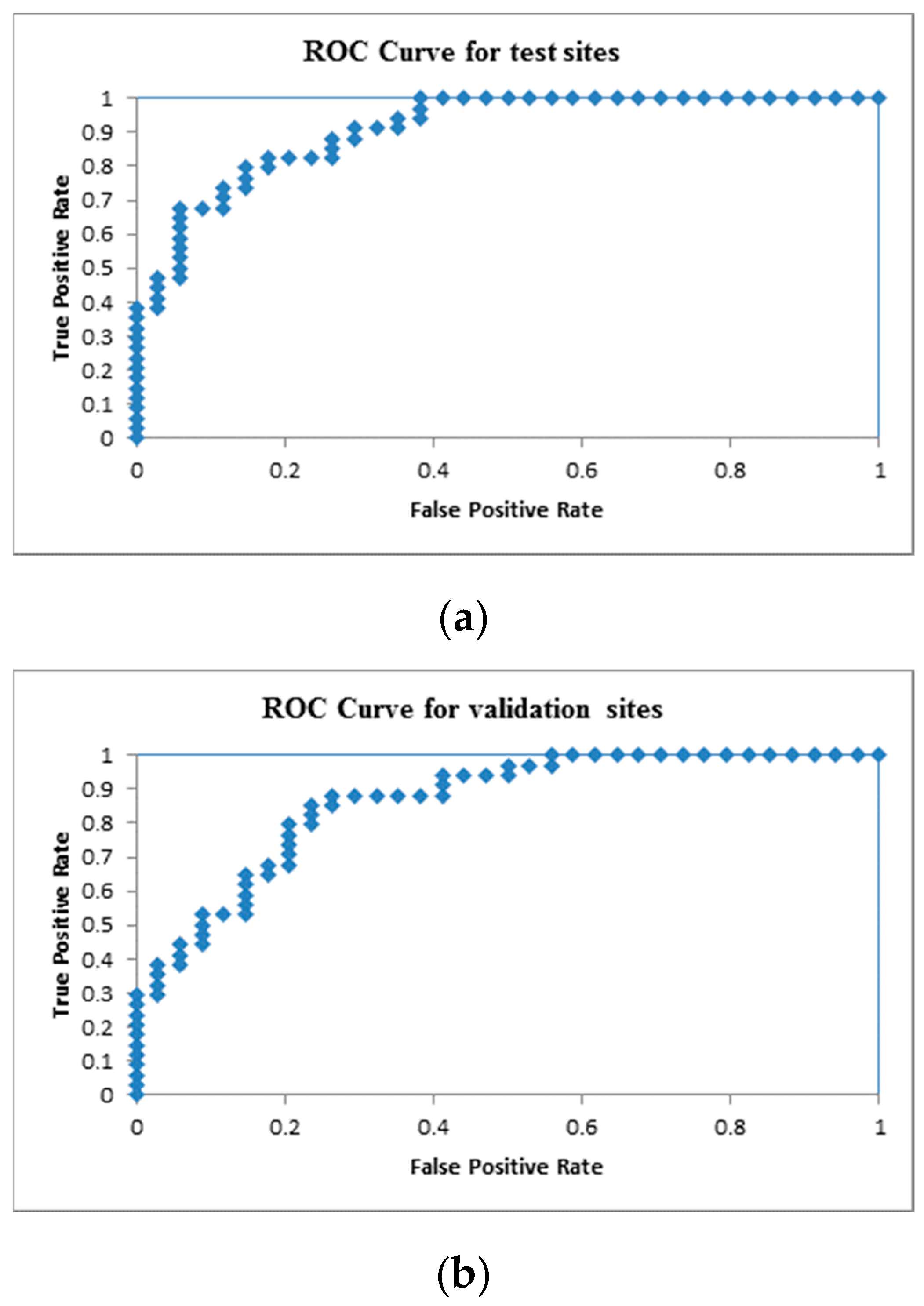
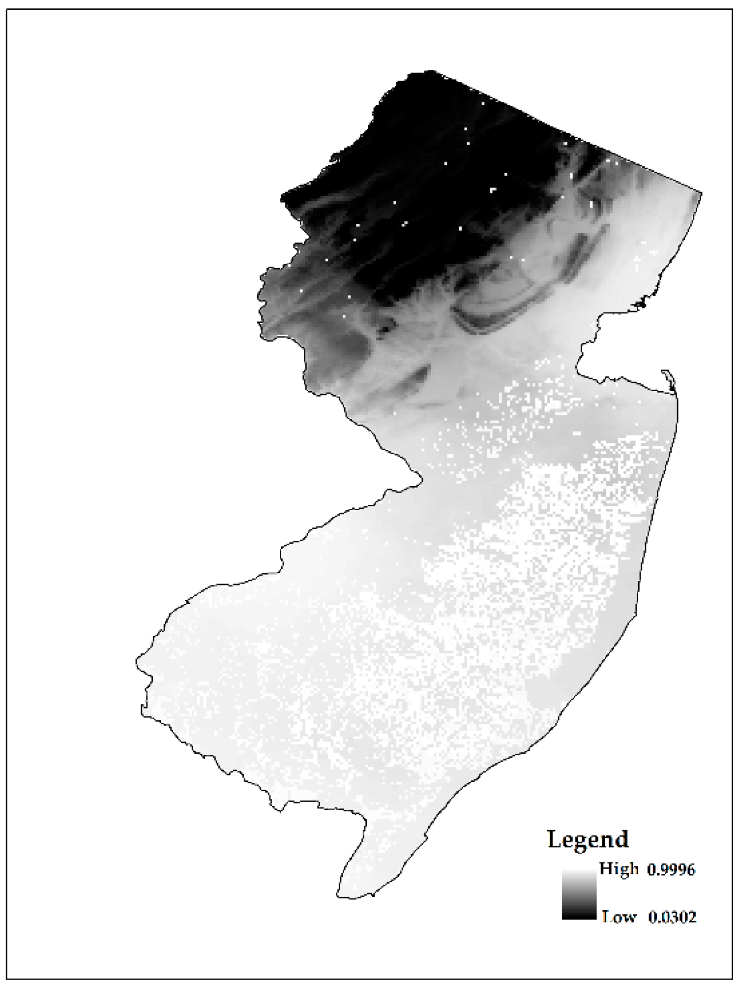
3. Results and Discussion

After running the binary logistic regression, results related to datasets training sites used to test the model and results used for validation were presented using tables and graphs. We performed several statistical tests following the recommendation by the American Statisticians Association (ASA), who advised that conclusions based solely on the results from p-values may not be sufficient and that some statisticians prefer to supplement p-values with other approaches [69]. For instance, concerning the earlier mentioned classification table (Table 1), our results are displayed in Table 2 and Table 3.
The datasets training set model accurately predicted the presence of E. Curvula by 82.35%, while the validation model predicted by 79.41%. The overall accuracy, using the interpretation scheme from Table 1, is 80.88% for the datasets training model and 77.94% for the validation model. Based on the accuracy of these relatively close results, we could conclude that the logistic regression model was a good fit for such this study.
We also analyzed the overall performance of the model by looking at the Chi-squares and p-values of the datasets training set model compared to the validation-sites model (Table 4).
In both cases represented in Table 4, the results show once again that the logistic regression model is a good fit in the analysis of the distribution of E. Curvula in the state of New Jersey.
We further analyzed results from the Hosmer–Lemeshow (HL) test to determine the goodness of fit of the logistic regression model on the two sites (Table 5).
The HL statistic for the datasets training set’s model was 46.371 and the p-value 0.968 > 0.05, and for the validation sites, it was 59.098 and the p-value 0.714 > 0.05. In both cases, it resulted in a non-significant HL test indicating that the logistic model was a good fit.
The accuracy of the model was further evaluated using the area under the curve (AUC) values from the relative operating characteristic (ROC) curve (Figure 2). Bazzichetto et al. [35], Hosmer and Lemeshow [51], Pearce and Ferrier [60], and Zaiontz [52], have suggested that the closer an AUC value was to 1 the better was the model fit and the better was the ability of the model to discriminate between success and failure. The AUC value for the datasets training points was 0.907, and for the validation sites, it was 0.862. Hence, we concluded that our model was a good fit and it had an excellent discrimination capability.
Results from Table 6 show the significance of each selected variable to the fitness of the model. All the variables had p-values less than 0.05.
A map of probability of occurrence of E. curvula (Figure 3) was created using the logistic function from Equation (3). Higher probability values designated areas where the presence of E. curvula was very likely to be present (lighter gray tone on the map), while lower values indicated the least likely areas to find the species (darker gray tone on the map).
E. curvula has not spread throughout the entire state of New Jersey. Soil and climate parameters, as demonstrated by the predictive model, have helped to identify its range of growth and adaptation. Results from the spatial analysis of the distribution of E. curvula revealed that the species is mostly concentrated in the southern part of the state. The eight counties where the species has been spotted are all within the Coastal Plain Physiographic Province of New Jersey (Atlantic County, Burlington County, Camden County, Cape May County, Cumberland County, Gloucester County, Middlesex County, and Salem County) [70]. While this physiographic province occupies three-fifths of New Jersey, and it is part of a much larger system that stretches over 3540 km from Cape Cod, Massachusetts, to the Mexican border [70,71]. Much of the soils in this province are sandy, dry, and acidic, with low fertility that makes it unconducive to agricultural use aside from blueberries and cranberries. Therefore, large areas within the Coastal Plain Province remain undeveloped. In addition to the soil quality being consistent with E. curvula locations noted in the literature, the climatic conditions in southern New Jersey may be relatively similar to the ones characterized by previous studies that documented environmental conditions [38,39,40,47,48] as ideal for the species to thrive.
Whereas most invasive plant species thrive in the highly disturbed ecosystems found in urban and suburban areas, the results from this study showed that a high human population density might not be associated with a high concentration of E. curvula. Two counties (Atlantic County and Burlington Counties) where the species was found in its highest abundance had a relatively low population density. On the other hand, counties with the highest population density including Union, Essex, and Hudson in the New York Metropolitan Area, do not have any documented occurrences of E. curvula. Densely populated areas have more impervious areas that inhibit the growth of the species as opposed to areas with more open space and the presence of soil. Many reported cases were found in ecologically-intact forests that are protected by the State, Federal Government, or the New Jersey Conservation Foundation (e.g., Wharton State Forest, Edwin B. Forsythe Wildlife Refuge, Higbee Beach Wildlife Management Area, and Franklin Parker Preserve).
This study found that the road network, in combination with other environmental factors, plays a role in species dispersal in New Jersey. In addition to climate restriction, all of the reported cases were found only within the 500 m-buffer zones of the roads (Figure 4). Cars or trucks appear to be the mechanism of dispersal. However, the road-speed limit has some impacts on the species dispersal because local roads (town toads) that have a 25-miles limit do not have any E. curvula species. More than half of reported cases were found along US and State highways (US Highway 322, US Highway 40, State Route 168, State Routes 72 and 73). The remaining identified species were located along county or rural roads. The actual species spatial distribution did not show its presence within its 500-meter buffer zone even though it was first planted along the Garden State Parkway [41]. Vehicle tires may have been playing a dominant role in the seed dispersal as opposed to other suggested dispersal mechanisms [72].
In southern New Jersey, the species grows primarily on sandy soil but has been documented on a wide range of soils. Using the United States Department of Agriculture classification scheme [73], the species was found on Lakehurst series soil and Atsion sand series. These soil types consist of deep, moderately well, or somewhat poorly drained soils and are typically found in lowland or upland areas. It also grows on Downer and Manahawkin sand series—a loamy type of sand that can be found on 0 to 5 percent slopes. Even though previous studies have indicated that the species has adapted to survive in coarse-textured soils, the results from the logistic model have shown that it has not adapted to surviving and growing in fine-textured soils in our study area.
The increasing spread of invasive plants is a critical driver of global environmental change [34]. Conservation managers recognize that predicting infestations of invasive plants will help in planning for long-term environmental management [36]. Over the past decades, remote sensing has improved our understanding of the drivers, processes, and effects of plant invasions through features such as identifying invaded ecosystems, predicting the distributions of invasive species, and in comprehending landscape invasibility and associated ecological impacts [34]. In this study, we have offered an additional avenue of prediction. While this study focused on one invasive grass species, we believe that the methods of incorporating readily available GIS data into a logistic regression model can serve as a reliable tool to identify and predict the spatial occurrence of other invasive plants.
E. curvula can spread throughout non-planted sites, but the variables highlighted throughout this study control its distribution. Predictive models, such as logistic regression, can be built to predict its distribution. Even though some studies have suggested the efficiency of prioritizing the removal of low-density subpopulations of invasive species [74], we believe that it is cost-effective to concentrate on the southern end of New Jersey, where it is likely to be found as ascertained by the logistic regression model [75]. Out of the four original counties [41], today the species is not found in Ocean County and Monmouth County. It has spread mostly west into new counties, including Camden, Cape May, Cumberland, Gloucester, Salem, and Middlesex. However, more than 75% of newly discovered plants are still located in the Atlantic and Ocean Counties. Even though E. curvula has invaded new soil types, the species has been predicted to grow mostly on preferred soil types. The road network has been the principal route of its dispersal. For its eradication, attention must be paid to areas along the roads and in forested or protected environments.
As GIS and remote sensing technology continues to develop, we will see an increased effort to use these tools as predictors of invasion and to support management decision making. Here we present one such model that land managers can adopt. The next step is to bridge the divide between model theory and management practices in the development of efficient conservation solutions [35].

Author Contributions

Conceptualization, K.I.N.; Formal analysis, K.I.N.; Funding acquisition, D.S.; Investigation, K.I.N.; Methodology, K.I.N.; Resources, D.S.; Validation, K.I.N.; Visualization, K.I.N.; Writing—original draft, K.I.N.; Writing—review & editing, D.S.

Funding

This research received no specific grant from any funding agency, commercial, or not-for-profit sectors. Support for the publication of this paper was provided by the Dean of the College of Natural, Applied and Health Sciences at Kean University.

Conflicts of Interest

The authors declare no conflict of interest.

References

  1. Mack, R.N.; Erneberg, M. The United States Naturalized Flora: Largely the Product of Deliberate Introductions. Ann. Mo. Bot. Gard. 2002, 89, 176–189. [Google Scholar] [CrossRef]
  2. Mack, R.N.; Lonsdale, W.M. Humans as Global Plant Dispersers: Getting More Than We Bargained For. BioScience 2001, 51, 95–102. [Google Scholar] [CrossRef] [Green Version]
  3. Mooney, H.A.; Cleland, E.E. The Evolutionary Impact of Invasive Species. Proc. Natl. Acad. Sci. USA 2001, 98, 5446–5451. [Google Scholar] [CrossRef] [PubMed] [Green Version]
  4. Reichard, S.H.; White, P. Horticulture as a Pathway of Invasive Plant Introductions in the United States. BioScience 2001, 51, 103–113. [Google Scholar] [CrossRef]
  5. Rossman, A.Y. A Special Issue on Global Movement of Invasive Plants and Fungi. BioScience 2001, 51, 93–94. [Google Scholar] [CrossRef] [Green Version]
  6. Swearingen, J.; Bargeron, C. Invasive Plant Atlas of the United States. 2016. Available online: http://www.invasiveplantatlas.org/ (accessed on 24 April 2016).
  7. Lehan, N.E.; Murphy, J.R.; Thorburn, L.P.; Bradley, B.A. Accidental Introductions Are an Important Source of Invasive Plants in the Continental United States. Am. J. Bot. 2013, 100, 1287–1293. [Google Scholar] [CrossRef]
  8. Allen, J.M.; Leininger, T.J.; Hurd, J.D.; Civco, D.L.; Gelfand, A.E.; Silander, J.A. Socioeconomics Drive Woody Invasive Plant Richness in New England, USA through Forest Fragmentation. Landsc. Ecol. 2013, 28, 1671–1686. [Google Scholar] [CrossRef]
  9. Staudhammer, C.L.; Escobedo, F.J.; Holt, N.; Young, L.J.; Brandeis, T.J.; Zipperer, W. Predictors, Spatial Distribution, and Occurrence of Woody Invasive Plants in Subtropical Urban Ecosystems. J. Environ. Manag. 2015, 155, 97–105. [Google Scholar] [CrossRef]
  10. Richardson, D.M.; Rejmánek, M. Trees and Shrubs as Invasive Alien Species-a Global Review: Global Review of Invasive Trees & Shrubs. Divers. Distrib. 2011, 17, 788–809. [Google Scholar] [CrossRef]
  11. Vicente, J.R.; Fernandes, R.F.; Randin, C.F.; Broennimann, O.; Gonçalves, J.; Marcos, B.; Pôças, I.; Alves, P.; Guisan, A.; Honrado, J.P. Will Climate Change Drive Alien Invasive Plants into Areas of High Protection Value? An Improved Model-Based Regional Assessment to Prioritise the Management of Invasions. J. Environ. Manag. 2013, 131, 185–195. [Google Scholar] [CrossRef]
  12. New Jersey Invasive Species Council. New Jersey Strategic Management Plan for Invasive Species. Available online: https://www.nj.gov/dep/njisc/docs/Final%20NJ%20Strategic%20Management%20Plan%20for%20Invasive%20Species%2011.09.pdf (accessed on 24 April 2016).
  13. Brown, A. Ballast Plants in and Near New York City. Bull. Torrey Bot. Club 1880, 7, 122–126. [Google Scholar] [CrossRef]
  14. Martindale, I.C. The Introduction of Foreign Plants. Bot. Gaz. 1876, 2, 55–58. [Google Scholar] [CrossRef]
  15. Snyder, D.; Kaufman, S.R. An Overview of Nonindigenous Plant Species in New Jersey; New Jersey Department of Environmental Protection, Division of Parks and Forestry, Office of Natural Lands Management, Natural Heritage Program: Trenton, NJ, USA, 2004.
  16. New Jersey Invasive Species Strike Team. New Jersey Invasive Species Strike Team. Available online: http://njisst.org (accessed on 15 September 2016).
  17. Beck, K.G.; Zimmerman, K.; Schardt, J.D.; Stone, J.; Lukens, R.R.; Reichard, S.; Randall, J.; Cangelosi, A.A.; Cooper, D.; Thompson, J.P. Invasive Species Defined in a Policy Context: Recommendations from the Federal Invasive Species Advisory Committee. Invasive Plant Sci. Manag. 2008, 1, 414–421. [Google Scholar] [CrossRef]
  18. National Invasive Species Council. 2008–2012 National Invasive Species Management Plan. Available online: https://www.doi.gov/sites/doi.gov/files/migrated/invasivespecies/upload/2008-2012-National-Invasive-Species-Management-Plan.pdf (accessed on 24 April 2016).
  19. Richardson, D.M.; Pyšek, P.; Carlton, J.T. A Compendium of Essential Concepts and Terminology in Invasion Ecology. In Fifty Years of Invasion Ecology; Richardson, D.M., Ed.; Wiley-Blackwell: Oxford, UK, 2010; pp. 409–420. [Google Scholar] [CrossRef]
  20. Richardson, D.M.; Pysek, P.; Rejmanek, M.; Barbour, M.G.; Panetta, F.D.; West, C.J. Naturalization and Invasion of Alien Plants: Concepts and Definitions. Divers. Distrib. 2000, 6, 93–107. [Google Scholar] [CrossRef]
  21. Daehler, C.C. Performance Comparisons of Co-Occurring Native and Alien Invasive Plants: Implications for Conservation and Restoration. Annu. Rev. Ecol. Evol. Syst. 2003, 34, 183–211. [Google Scholar] [CrossRef]
  22. Sakai, A.K.; Allendorf, F.W.; Holt, J.S.; Lodge, D.M.; Molofsky, J.; With, K.A.; Baughman, S.; Cabin, R.J.; Cohen, J.E.; Ellstrand, N.C.; et al. The Population Biology of Invasive Species. Annu. Rev. Ecol. Syst. 2001, 32, 305–332. [Google Scholar] [CrossRef] [Green Version]
  23. Davis, M.A.; Grime, J.P.; Thompson, K. Fluctuating Resources in Plant Communities: A General Theory of Invasibility. J. Ecol. 2000, 88, 528–534. [Google Scholar] [CrossRef] [Green Version]
  24. Funk, J.L. Differences in Plasticity between Invasive and Native Plants from a Low Resource Environment. J. Ecol. 2008, 96, 1162–1173. [Google Scholar] [CrossRef]
  25. Funk, J.L.; Vitousek, P.M. Resource-Use Efficiency and Plant Invasion in Low-Resource Systems. Nature 2007, 446, 1079–1081. [Google Scholar] [CrossRef]
  26. Nicotra, A.B.; Davidson, A. Adaptive Phenotypic Plasticity and Plant Water Use. Funct. Plant Biol. 2010, 37, 117–127. [Google Scholar] [CrossRef]
  27. Pyšek, P.; Richardson, D.M. Invasive Species, Environmental Change and Management, and Health. Annu. Rev. Environ. Resour. 2010, 35, 25–55. [Google Scholar] [CrossRef] [Green Version]
  28. Pyšek, P.; Richardson, D.M. Traits Associated with Invasiveness in Alien Plants: Where Do We Stand? In Biological Invasions; Nentwig, W., Ed.; Springer: Berlin/Heidelberg, Germany, 2007; Volume 193, pp. 97–125. [Google Scholar] [CrossRef]
  29. Werner, C.; Zumkier, U.; Beyschlag, W.; Máguas, C. High Competitiveness of a Resource Demanding Invasive Acacia under Low Resource Supply. Plant Ecol. 2010, 206, 83–96. [Google Scholar] [CrossRef]
  30. Whitney, K.D.; Gabler, C.A. Rapid Evolution in Introduced Species, ‘Invasive Traits’ and Recipient Communities: Challenges for Predicting Invasive Potential: Evolution and Invasion Predictions. Divers. Distrib. 2008, 14, 569–580. [Google Scholar] [CrossRef]
  31. Firn, J. African lovegrass in Australia: A valuable pasture species or embarrassing invader? Tropical Grasslands 2009, 43, 86–97. [Google Scholar]
  32. Han, Y.; Buckley, Y.M.; Firn, J. An Invasive Grass Shows Colonization Advantages over Native Grasses under Conditions of Low Resource Availability. Plant Ecol. 2012, 213, 1117–1130. [Google Scholar] [CrossRef]
  33. United States Congress, Office of Technology Assessment. Harmful Non-Indigenous Species in the United States; OTA-F-565; U.S. Government Printing Office: Washington, DC, USA, 1993; p. 391. Available online: https://govinfo.library.unt.edu/ota/Ota_1/DATA/1993/9325.PDF (accessed on 15 September 2016).
  34. Vaz, A.S.; Alcaraz-Segura, D.; Campos, J.C.; Vicente, J.R.; Honrado, J.P. Managing Plant Invasions through the Lens of Remote Sensing: A Review of Progress and the Way Forward. Sci. Total Environ. 2018, 642, 1328–1339. [Google Scholar] [CrossRef] [PubMed]
  35. Bazzichetto, M.; Malavasi, M.; Barták, V.; Acosta, A.T.R.; Moudrý, V.; Carranza, M.L. Modeling Plant Invasion on Mediterranean Coastal Landscapes: An Integrative Approach Using Remotely Sensed Data. Landsc. Urban Plan. 2018, 171, 98–106. [Google Scholar] [CrossRef]
  36. Iacona, G.; Price, F.D.; Armsworth, P.R. Predicting the Presence and Cover of Management Relevant Invasive Plant Species on Protected Areas. J. Environ. Manag. 2016, 166, 537–543. [Google Scholar] [CrossRef] [Green Version]
  37. Barbosa, F.G. The Future of Invasive African Grasses in South America under Climate Change. Ecol. Inform. 2016, 36, 114–117. [Google Scholar] [CrossRef]
  38. Gucker, C.L. Eragrostis Curvula. In Fire Effects Information System; USDA Forest Service, Rocky Mountain Research Station, Fire Sciences Laboratory: Missoula, MT, USA, 2009. Available online: https://www.fs.fed.us/database/feis/plants/graminoid/eracur/all.html (accessed on 28 May 2016).
  39. Peterson, P.M. Eragrostis. In Flora of North America North of Mexico; Magnoliophyta: Commelinidae (in Part): Poaceae, Part 2; Barkworth, M.E., Capels, K.M., Long, S., Piep, M.B., Eds.; Oxford University Press: New York, NY, USA, 2003; Volume 25, pp. 65–105. [Google Scholar]
  40. Skerman, P.J.; Cameron, D.G.; Riveros, F. Tropical Forage Legumes, 2nd ed.; Food and Agriculture Organization of the United Nations: Rome, Italy, 1988. [Google Scholar]
  41. Fairbrothers, D.E. Naturalization of Eragrostis Curvula (Weeping Lovegrass) in New Jersey. Bull. Torrey Bot. Club 1960, 87, 216. [Google Scholar] [CrossRef]
  42. New Jersey Department of Transportation (NJDOT). Statewide Capital Investment Strategy Fy 2013–2022. Available online: http://www.njleg.state.nj.us/OPI/Reports_to_the_Legislature/transportation_capital_investment_strategy_FY2013_2022.pdf (accessed on 15 September 2016).
  43. Colom, M.R.; Vazzana, C. Photosynthesis and PSII Functionality of Drought-Resistant and Drought-Sensitive Weeping Lovegrass Plants. Environ. Exp. Bot. 2003, 49, 135–144. [Google Scholar] [CrossRef]
  44. Mack, M.C.; D’Antonio, C.M. Impacts of Biological Invasions on Disturbance Regimes. Trends Ecol. Evol. 1998, 13, 195–198. [Google Scholar] [CrossRef]
  45. D’Antonio, C.M.; Vitousek, P.M. Biological Invasions by Exotic Grasses, the Grass/Fire Cycle, and Global Change. Annu. Rev. Ecol. Syst. 1992, 23, 63–87. [Google Scholar] [CrossRef]
  46. Skerman, P.J.; Riveros, F. Tropical Grasses; FAO Plant Production and Protection Series; Food and Agriculture Organization of the United Nations; UNIPUB: Rome, Italy; Laham, MD, USA, 1990. [Google Scholar]
  47. Cox, J.R.; Martin, M.H. Effects of Planting Depth and Soil Texture on the Emergence of Four Lovegrasses. J. Range Manag. 1984, 37, 204–205. [Google Scholar] [CrossRef]
  48. Cox, J.R.; Martin-R, M.H.; Ibarra-F, F.A.; Fourie, J.H.; Rethman, J.F.G.; Wilcox, D.G. The Influence of Climate and Soils on the Distribution of Four African Grasses. J. Range Manag. 1988, 41, 127–139. [Google Scholar] [CrossRef] [Green Version]
  49. Dahl, B.E.; Cotter, P.F.; Wester, D.B.; Britton, C.M. Grass Seeding in West Texas. Noxious Brush Weed Control Range Wildl. Manag. 1986, 17, 8–15. [Google Scholar]
  50. Crider, F.J. Three Introduced Lovegrasses for Soil Conservation; U.S. Dept. of Agriculture: Washington, DC, USA, 1945.
  51. Hosmer, D.W.; Lemeshow, S. Applied Logistic Regression: Hosmer/Applied Logistic Regression; John Wiley & Sons, Inc.: Hoboken, NJ, USA, 2000. [Google Scholar] [CrossRef]
  52. Zaiontz, C. Real Statistics Using Excel. Available online: http://www.real-statistics.com (accessed on 10 February 2017).
  53. Ludlum, D.M. The New Jersey Weather Book; Rutgers University Press: New Brunswick, NJ, USA, 1983. [Google Scholar]
  54. Office of the New Jersey State Climatologist. Climate Information. Available online: https://climate.rutgers.edu/stateclim/?section=njcp&target=NJCoverview (accessed on 10 February 2017).
  55. US Census Bureau 2016. Annual Estimates of the Resident Population: 1 April 2010 to 1 July 2016. Available online: https://factfinder.census.gov/faces/tableservices/jsf/pages/productview.xhtml?src=bkmk (accessed on 10 February 2017).
  56. James, G.; Witten, D.; Hastie, T.; Tibshirani, R. An Introduction to Statistical Learning: With Applications in R; Springer: New York, NY, USA, 2013; Available online: https://www.academia.edu/36691506/An_Introduction_to_Statistical_Learning_Springer_Texts_in_Statistics_An_Introduction_to_Statistical_Learning (accessed on 7 September 2017).
  57. Ekström, M.; Esseen, P.-A.; Westerlund, B.; Grafström, A.; Jonsson, B.G.; Ståhl, G. Logistic Regression for Clustered Data from Environmental Monitoring Programs. Ecol. Inform. 2018, 43, 165–173. [Google Scholar] [CrossRef]
  58. Goslee, S.C.; Beck, K.G.; Peters, D.P.C. Distribution of Russian Knapweed in Colorado: Climate and Environmental Factors. J. Range Manag. 2003, 56, 206. [Google Scholar] [CrossRef]
  59. Mansourian, S.; Darbandi, E.I.; Rashed Mohassel, M.H.; Rastgoo, M.; Kanouni, H. Comparison of Artificial Neural Networks and Logistic Regression as Potential Methods for Predicting Weed Populations on Dryland Chickpea and Winter Wheat Fields of Kurdistan Province, Iran. Crop Prot. 2017, 93, 43–51. [Google Scholar] [CrossRef]
  60. Pearce, J.; Ferrier, S. Evaluating the Predictive Performance of Habitat Models Developed Using Logistic Regression. Ecol. Model. 2000, 133, 225–245. [Google Scholar] [CrossRef] [Green Version]
  61. Reese, G.C.; Wilson, K.R.; Hoeting, J.A.; Flather, C.H. Factors Affecting Species Distribution Predictions: A Simulation Modeling Experiment. Ecol. Appl. 2005, 15, 554–564. [Google Scholar] [CrossRef] [Green Version]
  62. New Jersey Office of GIS Open Data. New Jersey Road Centerlines. Available online: http://njogis-newjersey.opendata.arcgis.com/datasets/new-jersey-road-centerlines (accessed on 24 April 2016).
  63. US Census Bureau. 2014 TIGER/Line Shapefiles (Machine-Readable Data Files)/Prepared by the U.S. Census Bureau, 2014 Economic and Statistics. 2016. Available online: https://www.census.gov/geographies/mapping-files/time-series/geo/tiger-line-file.2014.html (accessed on 24 April 2016).
  64. US Census Bureau 2016. Primary and Secondary Roads. Available online: https://www.census.gov/geo/maps-data/data/tiger.html (accessed on 24 April 2016).
  65. U.S. Department of Agriculture (USDA). National Geospatial Center of Excellence (NGCE)|NRCS. Available online: https://www.nrcs.usda.gov/wps/portal/nrcs/main/national/ngce/ (accessed on 24 April 2016).
  66. Soil Survey Staff. Natural Resources Conservation Service, United States Department of Agriculture. Web Soil Survey. Available online: https://websoilsurvey.nrcs.usda.gov/ (accessed on 12 April 2016).
  67. PRISM Climate Group, Oregon State U. Available online: http://prism.oregonstate.edu/ (accessed on 7 September 2017).
  68. U.S. Geological Survey, The National Map, 3DEP Products and Services: The National Map, 3D Elevation Program Web Page. Available online: https://www.usgs.gov/core-science-systems/ngp/3dep (accessed on 12 April 2016).
  69. Wasserstein, R.L.; Lazar, N.A. The ASA Statement on p -Values: Context, Process, and Purpose. Am. Stat. 2016, 70, 129–133. [Google Scholar] [CrossRef] [Green Version]
  70. Physiographic Provinces of New Jersey. Available online: https://rucore.libraries.rutgers.edu/rutgers-lib/18149/ (accessed on 28 September 2019).
  71. Coastal Plain Province (U.S. National Park Service). Available online: https://www.nps.gov/articles/coastalplain.htm (accessed on 28 September 2019).
  72. Clarke, S.; French, K. Germination Response to Heat and Smoke of 22 Poaceae Species from Grassy Woodlands. Aust. J. Bot. 2005, 53, 445. [Google Scholar] [CrossRef]
  73. U.S. Department of Agriculture (USDA). Field Guide for Managing Lehmann and Weeping Lovegrasses in the Southwest. Available online: https://www.fs.usda.gov/Internet/FSE_DOCUMENTS/stelprdb5410118.pdf (accessed on 24 April 2016).
  74. Taylor, C.M.; Hastings, A. Finding Optimal Control Strategies for Invasive Species: A Density-Structured Model for Spartina Alterniflora: Optimal Control Strategies for an Invasive Grass. J. Appl. Ecol. 2004, 41, 1049–1057. [Google Scholar] [CrossRef]
  75. Giljohann, K.M.; Hauser, C.E.; Williams, N.S.G.; Moore, J.L. Optimizing Invasive Species Control across Space: Willow Invasion Management in the Australian Alps: Spatial Allocation of Invasive Species Control. J. Appl. Ecol. 2011, 48, 1286–1294. [Google Scholar] [CrossRef] [Green Version]
Figure 1. Study area: The state of New Jersey.
Environments 06 00125 g001
Figure 2. Relative operating characteristic (ROC) curves for the datasets training sites (a) and validation sites (b).
Environments 06 00125 g002
Figure 3. Probability of occurrence of Eragrostis curvula.
Environments 06 00125 g003
Figure 4. Distribution of Eragrostis curvula and the main road network in New Jersey.
Environments 06 00125 g004
Table 1. Classification table [52].
Number of CasesSuc-ObsFail-ObsTotal Predicted
Suc-PredTPFPPP
Fail-PredFNTNPN
TotalOPONTO
In Table 1, Suc-Pred = Successes predicted, Fail-Pred = Failures predicted, Suc-Obs = Successes observed, Fail-Obs = Failures observed, TP = True Positives, FP = False Positives, TN = True Negatives, FN = False Negatives, PP = predicted positive = TP + FP, PN = predicted negative = FN + TN, OP = observed positive = TP + FN, ON = observed negative = FP + TN and TO = the total sample size = TP + FP + FN + TN. The overall accuracy ((TP + TN)/TO) is a measure of the fit of the logistic regression model.
Table 2. The number of successes/failures predicted by the logistic regression model compared to the number observed using the test sites.
Suc-Obs
Presence E. Curvula
Fail-Obs
Absence E. Curvula
Total
Suc-Pred28735
Fail-Pred62733
Total343468
Accuracy0.8235290.7941180.808824
Table 3. The number of successes/failures predicted by the logistic regression model compared to the number observed using the validation sites.
Suc-Obs
Presence E. Curvula
Fail-Obs
Absence E. Curvula
Total
Suc-Pred27835
Fail-Pred72633
Total343468
Accuracy0.7941180.7647060.779412
Table 4. Model comparison using the Chi Square.
Datasets Training Set ModelValidation Set Model
LL0−47.134−47.134
LL1−24.8012−31.7043
Chi Square44.6655830.85932
df44
p-value4.67 × 10−93.27 × 10⁻⁶
alpha0.050.05
significanceyesyes
LL0 refers to a log-likelihood model with only the intercept b0 and no other coefficients. LL1 refers to the full log-likelihood model. df refers to the degrees of freedom.
Table 5. Model comparison based on Hosmer–Lemeshow test.
Datasets Training Set ModelValidation Set Model
Hosmer-Lemeshow46.3712359.09845
df6666
p-value0.9682340.713769
alpha0.050.05
significancenono
Table 6. Logistic regression parameters for datasets training sites including the intercept, their coefficients, standard errors (s.e.), p = values, and their confidence intervals.
Coeff bs.e.Waldp-valueexp(b)LowerUpper
Intercept−22.359323.462280.9081920.3405951.95 × 10−10
Mean annual temperature3.4159981.2386027.606270.00581730.447332.686886345.0239
Soil classes2.0151380.643789.7979380.0017477.5017642.12410926.49415
Precipitation−0.021050.012942.6450390.0338740.9791750.9546531.004326
Distance away from road−6.2 × 10−53.12 × 10−53.8805230.0488490.9999380.9998771

